Post Newtonian SPH

Abstract

We introduce an adaptation of the well known Tree+SPH numerical scheme to Post Newtonian (PN) hydrodynamics and gravity. Our code solves the (0+1+2.5)PN equations. These equations include Newtonian hydrodynamics and gravity (0PN), the first order relativistic corrections to those (1PN) and the lowest order gravitational radiation terms (2.5PN). We test various aspects of our code using analytically solvable test problems. We then proceed to study the 1PN effects on binary neutron star coalescence by comparing calculations with and without the 1PN terms. We find that the effect of the 1PN terms is rather small. The largest effect arises with a stiff equation of state for which the maximum rest mass density increases. This could induce black hole formation. The gravitational wave luminosity is also affected.

1 Introduction

The development of numerical methods for the solutions of full 3D general relativistic hydrodynamic problems is still at a preliminary stage (Font et al., 1998). In the meanwhile, various approximate approaches to this problem have been attempted. Of these some include an approximation to the metric in the form of the conformal flatness condition (CFC) (Mathews & Wilson, 1997) or by using a Post-Newtonian (PN) formulation of the equations (Shibata et al., 1997; Oohara & Nakamura, 1997). Recently it has been suggested that at least in some cases these two approximations are of the same order of accuracy (Kley & Schäfer, 1999). In this work we set out to modify the popular Tree-SPH (Benz et al., 1990; Hernquist & Katz, 1989) numerical scheme formulated for Newtonian self gravitating hydrodynamic systems to work in the PN approximation. We need to adapt both parts of the Tree-SPH scheme - the tree code and the SPH. Our goal is to study the coalescence of binary neutron stars (BNS), an intrinsically 3D hydro+gravity problem, and to begin the exploration of the general relativistic effects which are important in this process.

Smooth Particle Hydrodynamics (SPH) is a Lagrangian, grid-less particle method for solving the hydrodynamic equations. It is this lack of a grid which makes SPH especially appealing for the efficient solution of complex 3D problems. SPH has been used in hydrodynamic simulations including gravity, magnetic fields and in special relativistic problems (Kheyfets et al., 1990; Siegler & Riffert, 1999). Laguna et al. (1993) have also implemented a fully general relativistic SPH with a fixed Kerr background. For a review on SPH techniques see Monaghan (1992) and Benz (1990). The Barnes-Hut Tree algorithm (Barnes & Hut, 1986) is a $O(N\log N)$ method for calculating gravitational forces between $N$ particles. It has been combined with SPH in order to get a powerful and efficient particle based gravity+hydro solver.

We combine the efficiency of the SPH approach with a PN formalism suggested by Blanchet et al. (1990) (BDS). The PN approximation to gravity involves expanding the relativistic equations with a small parameter $O(v^{2}/c^{2})$ where $v$ is a typical velocity in the system (thermal velocity, orbital velocity etc…). 1PN means we neglect all terms proportional to $v^{4}/c^{4}$ and higher. The 1PN approximation includes in the first order, many relativistic effects. The main shortcoming of the 1PN approximation is that it misses all effects which have to do with gravitational radiation. These effects appear only at the 2.5PN ($v^{5}/c^{5}$) order. The BDS formalism includes the Newtonian physics (0PN), the leading order PN effects (1PN) and the leading order gravitational radiation effects (2.5PN) in a self consistent way. It recasts the PN equations in a form similar to the Newtonian equations thus facilitating the adaptation of the Tree-SPH algorithm to solve this problem.

In this work we introduce the code and present code tests. We also use the code to simulate binary neutron star (BNS) coalescence in the (0+1+2.5)PN approximation and to compare these results to Newtonian simulations. In section 2 we introduce the numerical method. In section 3 we examine the results of various code tests. We present the results of the BNS coalescence simulation in section 4 and we conclude in section 5.

2 Numerical method

The BDS formalism recasts the (0+1+2.5)PN gravitation and hydrodynamic equations in a form resembling the Newtonian (0PN) equations. This enables the solution of these equations using methods adapted from Newtonian gravity (such as the Tree+SPH method we use here). The formalism reduces all the relativistic non-local equations to compact supported Poisson equations. The PN order of the various terms in the equations of motion can be read off their coefficients - 0PN terms have no coefficients, 1PN have coefficients proportional to $1/c^{2}$ and 2.5PN terms have coefficients proportional to $1/c^{5}$. This enables us to “turn off” various powers of the PN approximation by setting to zero the corresponding coefficients. We use this option later when making a (0+2.5)PN calculation.

The independent matter variables used are the following set: $\rho_{*}$ the coordinate rest mass density, $\varepsilon_{*}$ the coordinate specific internal energy and $\bf{w}$ the specific linear momentum. In fully relativistic terms these are defined as:

$$\rho_{*} = \sqrt{g}u^{0}\rho,$$ (1)

$$\varepsilon_{*} = \varepsilon(\rho_{*}),$$ (2)

$$w_{i} = \left(c^{2}+\varepsilon+p/\rho\right)\frac{u_{i}}{c},$$ (3)

where $\rho$ is the rest mass density, $\varepsilon(\rho)$ the specific energy, $p(\varepsilon,\rho)$ the pressure and $u^{\mu}$ the four-velocity (Greek indices run from 0 to 4, Latin indices from 1 to 3). The corresponding BDS variables are the above quantities neglecting all terms except 0PN, 1PN and 2.5PN. Using these variables the formalism yields an evolution system which consists of 9 Poisson equations and 8 hyperbolic equations (see Appendix A).

In the 0PN approximation ($c\rightarrow\infty$) $w_{i}=v^{i}$, $\rho_{*}$ is the mass density, the only needed potential is $U_{*}$, and we recover the known Newtonian equations of motion. From Eq. (A7) we have $Q^{[3]}_{ij}=d^{3}Q_{ij}/dt^{3}+O(1/c^{2})$, where $Q_{ij}$ is the quadropole moment, enabling us to compute the gravitational radiation luminosity of the system to lowest order as

$$L_{\rm GW}=\frac{1}{5}\frac{G}{c^{5}}Q^{[3]}_{ij}Q^{[3]}_{ij}.$$ (4)

The BDS equations are self-consistent as long as the system is only mildly relativistic. This can be characterized by noting that at least the parameters $\alpha/c^{2}$, $\beta/c^{2}$ and $\delta/c^{2}$ (Eq. A1, A2 and A3 respectively) must be small. This means that contrary to 0PN systems which are always self-consistent but can be physically wrong the 1PN system will cease to be self consistent at the time when its results are too far from the general relativistic results. This inconsistency can be understood as follows: given two functions expanded in a small parameter $\eta\ll 1$

$$f = f_{0}+f_{1}\eta+\ldots,$$ (5)

$$g = g_{0}+g_{1}\eta+\ldots,$$ (6)

the product of these functions is

$$fg=f_{0}g_{0}+(f_{0}g_{1}+f_{1}g_{0})\eta+(f_{0}g_{2}+2f_{1}g_{1}+f_{2}g_{0})\eta^{2}+\ldots.$$ (7)

If we choose to truncate the functions at the first order (setting $f_{i}=0$ for $i>1$) and indeed $\eta\ll 1$ then we can also neglect the $\eta^{2}$ terms in the product, but if $\eta\approx 1$, we will also need to take into consideration the $2f_{1}g_{1}\eta^{2}$ term in the product if we wish to be self-consistent (the approximation would break down in any case giving wrong results). Similarly in order to make the 1PN system self consistent we would need to add some 2PN terms to the equations complicating them even more. This is not the case if we wish to truncate the functions at the zero order ($f_{i}=0$ for $i>0$). Then we can consistently truncate the product also at the zero order. This explains the self-consistency of the Newtonian (0PN) approximation.

For the solution of the Poisson equations we used a Barnes-Hut tree (Barnes & Hut, 1986). The Barnes-Hut tree is a $O(N\log N)$ method commonly used for $N$-body gravitational force calculations. The principle behind the Barnes-Hut tree is that at a given position, the gravitational force from a cluster of distant particles can be approximated by using only global properties of the cluster - the monopole, dipole and quadrupole moments of the mass distribution. The Barnes-Hut tree provides a simple way to calculate these moments and to cluster the particles. It is remarkable that the same formalism can be used with minor modification to solve any compact supported elliptic equation. We adapt this method to solve a general compact supported elliptic equation (see Appendix B) and we use it here to solve numerically equations (A8)-(A12). In all our runs we set the tree accuracy parameter $\theta$ to 0.5. Gravitational softening was naturally incorporated by assigning particles with their respective SPH mass density in the gravitational calculations.

The evolution equations were solved using SPH, a Lagrangian particle based scheme for solving hydrodynamic problems. The use of SPH was facilitated by the similarity of the equations in the BDS formalism to the Newtonian equations (indeed this is the whole point in the BDS formalism). The particle mass used in Newtonian SPH was replaced by the conserved mass $m_{*}=\int d^{3}x\,\rho_{*}$ in our scheme. When using SPH Eq. A17 is automatically satisfied and only equations A18-A20 have to be solved. The use of SPH requires adding some artificial viscosity in order to resolve shocks. We use the standard artificial viscosity (e.g. Monaghan, 1992; Benz, 1990) consisting of a term analogous to bulk viscosity and a Von Neuman-Richtmyer artificial viscosity term.

We used a symmetrical form of the SPH equations which guarantees the exact conservation of the “momentum” $\int d^{3}x\,\rho_{*}w_{i}$ in the hydrodynamics section of the code. The momentum isn’t exactly conserved in the gravity section of the code because the tree algorithm introduces a small asymmetry into the forces. This problem arises also in Newtonian SPH calculations as well and it leads to spurious accelerations of the center of mass of the system. These acceleration are small for a typical Tree parameters (of the order of $10^{-6}$ compared to other accelerations in the system) and can be corrected by simply subtracting the center of mass acceleration from the particle accelerations at each time step.

For time integration we used a second order Runge-Kutta integrator with adaptive step size control. The step size was determined so that none of the integrated variables will change by more than a predetermined amount, set to 0.5% in all runs. In addition we check that the Courant condition is always satisfied. We did not implement single particle time steps. The simulations were run on standard Pentium II 450MHZ workstations and took about 255 hours of CPU time ($\sim 11$ days) each.

3 Code Tests

Numerous studies have been conducted on the capabilities and limitations of the SPH formalism (Hernquist & Katz, 1989; Davies et al., 1993; Lombardi et al., 1999). We have put our code through a suite of tests to insure that our implementation is correct and that it reproduces previously obtained results using available codes. Specifically we have compared the Newtonian (0PN) version to the Newtonian SPH code used in Davies et al. (1994). This comparison ensures the validity of the Newtonian part of our code. We devised other simple tests for the different PN aspects of the code - (0+1)PN hydrodynamics, gravitational radiation damping (2.5PN) and (0+1)PN hydrodynamics and gravity. These all have an analytical or easily obtainable result and take a reasonable time to run.

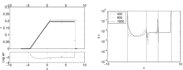
b

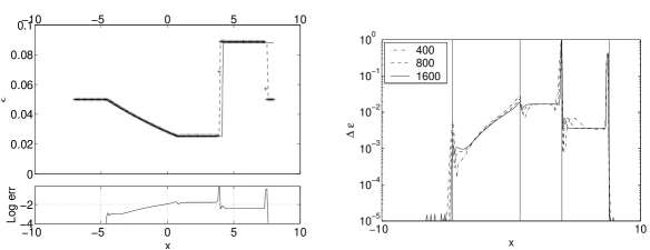
c

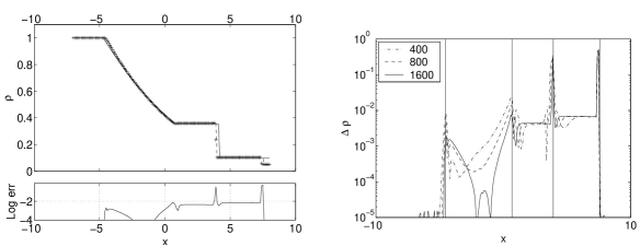
Figure 1: Shock tube results for a $\gamma=5/3$ gas. (a) The velocity. (b) The internal energy density $\varepsilon$. (c) The rest mass density $\rho$. Initial conditions were $\rho_{*l}=1$, $\rho_{*r}=0.05$, and $\varepsilon_{*}=0.05$ using 800 particles. On the left, each graph shows the Newtonian analytical results in a solid line, the relativistic analytical results in a dashed line and the (0+1)PN numerical points as crosses. Under each graph is the error in the (0+1)PN result as compared to the relativistic result. On the right the each graph shows the error relative to the analytic relativistic solution. The vertical lines mark the left edge of the rarefraction, the right edge of the rarefraction, the contact discontinuity and the shock going from left to right. The error is calculated for solutions with 400, 800 and 1600 particles. Except around the discontinuities the error converges to $\approx 10^{-2}$, which is the expected error resulting from neglecting 2PN and higher terms ($\varepsilon^{2}\approx\cdot 10^{-2}$).

(0+1)PN hydrodynamics (without gravity) were tested using the 1D shock tube problem. We have compared the results to both the Newtonian and the relativistic solutions (Taub, 1948; McKee & Colgate, 1973; Hawley et al., 1984). These tests were conducted with a 1D version of our code which differs from the 3D version used elsewhere in this paper only by the normalization of the SPH smoothing kernel. The results of the tests are presented in Figure 1. These tests demonstrate that our PN code gives better results than a Newtonian code for mildly relativistic problems, with shock velocities of $\sim 0.2c$. These conditions are at the upper limit of the validity of the (0+1)PN approximation as $\varepsilon\approx 0.1c^{2}$. We compare (0+1)PN calculation to the analytic Newtonian solution and the relativistic analytical solution. The error in the (0+1)PN velocity is smaller by an order of magnitude than the Newtonian error. This leads to a more accurate estimate of the shock’s position. The errors for the energy density and mass density are larger, but still better or comparable to the Newtonian error. We conclude that even in these extreme conditions for the (0+1)PN hydrodynamic approximation, it fares at least as well as Newtonian hydrodynamics, and is much better at estimating the velocity of the fluid. In all the quantities, the relative error of the (0+1)PN result as compared to the relativistic analytical solution is of the order of 1% except for single particles which reside at discontinuities. In Figure (1) we also show the convergence of the results. We show the relative error compared to the analytic relativistic results for different particle numbers. Except at the discontinuities the error relative to the (0+1)PN result converges to $\approx 10^{-2}$. The size of the zone around the discontinuities with a large error decreases when the number of particles increases, indicating, again, that the discontinuities affect only a fixed small ($\approx 10$), number of particles. The convergence of the error to $\approx 10^{-2}$ is consistent with the order of magnitude of the largest 2PN term - $\varepsilon^{2}/c^{4}$ which is the expected error of the (0+1)PN approximation. We point out that 3D tests of shocks with the particles positioned randomly, which are expected to model the conditions in a 3D run more realistically, give much poorer resolution (Rasio & Shapiro, 1991a).

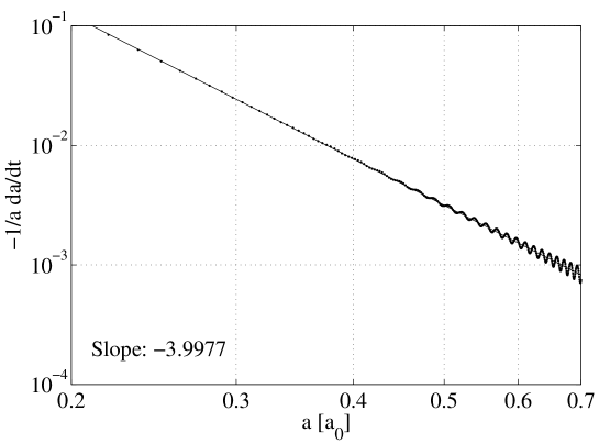
Figure 2: Results of (0+2.5)PN runs with point masses which check the accuracy of gravitational radiation damping: a plot of $-\dot{a}/a$ vs. $a$. The initial points with $a>0.7a_{0}$ (where $a_{0}$ is the initial separation) were excluded to allow for numerical relaxation. The expected slope is -4.

Gravitational radiation backreaction (the 2.5PN terms) was tested using two point masses in orbit. In this run, all the 1PN terms were discarded leaving only (0+2.5)PN terms. Since we used two point masses, hydrodynamics didn’t play any role in this test. The rate of change of the orbit’s radius was compared to the analytical result of $\dot{a}/a\propto-a^{-4}$ (see e.g. Shapiro & Teukolsky (1983), Chapter 16). Figure 2 depicts the results of this test. The two point masses were set initially in a Keplerian orbit. Since this is only an approximation to actual quasi-stationary orbits of (0+2.5)PN gravitation, a brief period of relaxation preceded the orbital decay after which the expected power law emerged.

The (0+1)PN gravity and hydrodynamics were tested using a static polytropic star with a polytropic index $\gamma=5/3$. Initial conditions were constructed using a (0+1)PN expansion of the Oppenheimer–Volkoff (OV) equations for a relativistic spherical star. We ran this test with two resolutions, 2151 and 5140 particles respectively, for approximately 50 hydrodynamic time scales (which we take to be $\sqrt{R^{3}/GM}$). for the initial conditions we use regularly placed unequal mass particles. The stars were constructed by placing the particles in a face-centred cubic (FCC) lattice, thus maximizing the number of neighbors each particle has. Using an iterative procedure, each particle is than assigned a mass so that the resulting density profile matches the OV density profile.

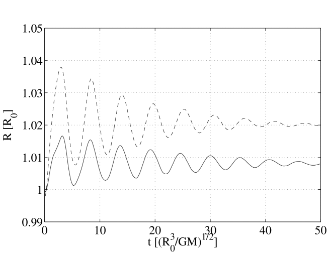
b

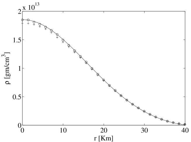
Figure 3: (0+1)PN $\gamma=5/3$ polytropic stars made out of 2151 and 5140 particles. The simulation ran for about 50 hydrodynamic time scales. The parameters of the star were $R_{0}=34$ Km and $M=0.49~{}{\rm M_{\odot}}$. (a) The radius inclosing 95% of the mass. The solid line and dashed line are for the 2151 and 5140 particle runs respectively. (b) Rest mass density profiles. The initial profile in a solid line and the final profiles of the 2151 and 5140 particle runs in crosses and circles respectively.

Figure 3a depicts the radius enclosing 95% of the mass. This radius oscillates with a decreasing amplitude converging to a constant value. There are less than 50 oscillation in the graphs since the oscillation period for these stars is some factor of order unity times $\sqrt{R^{3}/GM}$, which we take to be the hydrodynamical timescale. The oscillations are caused by several factors in the SPH algorithm. Every SPH particle adjusts it’s size $h$ so that it will have approximately 50 other particles as neighbors (within a sphere of radius $2h$). In our initial conditions all the particles have the same $h$, this causes the particles near the star’s surface to have only half the neighbors, and their $h$ is increased by the code. This in turn lowers the density and takes the star out of equilibrium. Another reason for the oscillations is that $\nabla P\neq 0$ on the boundary of the star due to numerical errors. Finally in the initial conditions the particles are positioned on a Cartesian grid which clearly conflicts with the spherical symmetry of the OV density profile assigned to them. The star begins to oscillate but the oscillations are damped by the artificial viscosity present in the SPH algorithm. The expected errors in all quantities (radius, central density, etc…) from the SPH discretisation error $(\langle h\rangle/R_{0})^{2}$ are 1.5% and 0.9% for the 2151 and 5140 particle runs respectively. As can be seen in Figure 3, the oscillations decrease when we increase the resolution. The final rest mass density, shown in Figure 3b, converges towards the analytical curve as the resolution increases.

4 PN BNS coalescence

BNS’s provide an excellent test-bed for gravitational and nuclear astrophysics. A binary pair of neutron stars will loose angular momentum and energy via gravitational wave emission as has been observed (see Taylor, 1994, and references therein). This process will ultimately lead to a coalescence of the two neutron stars. The gravitational waves emitted from the coalescence are expected to be observed by gravitational wave detectors coming on-line in the next decade, such as LIGO (Barish, 1998), VIRGO (Fidecaro & Collaboration, 1997), GEO (Hough et al., 1996) and TAMA (Kozai & Tama-300 Collaboration, 1999).

At the final stages of the coalescence the BNS system must be described using detailed 3D modeling of gravitational and hydrodynamic effects. This restricts the study of the last stages of coalescence to numerical methods. Many groups have performed numerical simulations using different approximations to this problem. Results have been obtained using Newtonian dynamics by Davies et al. (1994), Rasio & Shapiro (1995), Wang & Swesty (1997), Ruffert & Janka (1998) and Rosswog et al. (1999). Post Newtonian (PN) results have also been obtained by Shibata et al. (1997) and Oohara & Nakamura (1997). Recently an almost fully relativistic result was obtained by Mathews & Wilson (1997) who used the CFC approximation (although see Flanagan (1999) and Kley & Schäfer (1999) for cautionary remarks on the validity of this approximation).

Although sophisticated techniques were developed in order to obtain equilibrium binary configurations both in the (0+1)PN (Shibata, 1997, 1998) and general relativistic (Baumgarte et al., 1998) cases, converting the resulting density field into SPH particles is not a trivial task. Previous works using Newtonian SPH usually manufacture equilibrium configurations by relaxing the system in the co-rotating frame, in which the stars are stationary (e.g. Rasio & Shapiro, 1991b). This approach was unavailable to us because of the complicated nature of the (0+1+2.5)PN equations. Instead we assign two spherical stars with Keplerian velocity (as in Shibata et al. 1998), and after some oscillations the system settles down into a stationary state.

We model the binary NS system by two equal polytropes with zero spins relative to an inertial observer (For further discussion on the initial spins and their implications see Rosswog et al. (1999) and references therein). On top of this we made several other simplifying assumptions in our calculation which are already discussed in Davies et al. (1994), namely ignoring neutrino transport. The masses we use for each star are less than $\rm M_{\odot}$ for radii of about 30 Km. Although these parameters are far from realistic for NS’s, they allow us to investigate the effect of general relativity on the coalescence while still in the regime of applicability of the (0+1+2.5)PN approximation for the whole duration of the run. We compare the (0+1+2.5)PN results (hereafter denoted P) to (0+2.5)PN runs (hereafter denoted N) with the same mass and initial separation to highlight the 1PN effects. We make a total of 6 runs (3 pairs of P-N runs). The parameters for these different runs are summarized in Table 1.

Run	$\gamma$	M [$\rm M_{\odot}$]	$R_{*}$ [Km]		Particles	$m_{\rm esc}$ [$\rm M_{\odot}$] (# part.)
			P	N		P	N
1	$5/3$	0.52	29.8	33.9	4996	$<3.7\times 10^{-5}$ (0)	$<3.7\times 10^{-5}$ (0)
2	2.6	0.50	34.7	36.9	20562	$2.6\times 10^{-4}$ (8)	$6.9\times 10^{-4}$ (20)
3	2.6	0.92	30.5	35.6	18520	$<4.3\times 10^{-5}$ (0)	$4.5\times 10^{-4}$ (6)

Table 1: Summary of results and parameters for the various runs. M is the conserved mass per star, $R_{*}$ the radius encompassing 95% of the conserved mass of each star in the initial configuration, $m_{\rm esc}$ is the mass of unbound particles in the final configuration. The upper limits on $m_{\rm esc}$ are the masses of the lightest particles in the run.

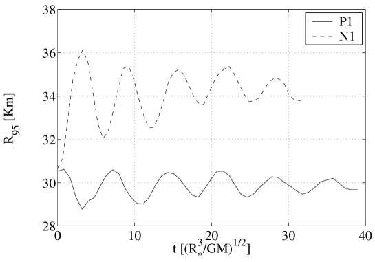
Figure 4: The radii of the stars as a function of time for the beginning of the P1 and N1 runs. The initial polytropes are static in the (0+1)PN approximation. The initial expansion in the N run reflects in the larger size of the N static polytrope. Based on this graph we take the radius of the P1 run to be 29.8Km and the radius of the N1 run to be 33.9Km. For the P1 run this is within 3% of the initial radius and for the N1 run this is 10% more than the initial radius. Note that in this graph the units are different than in all following graphs

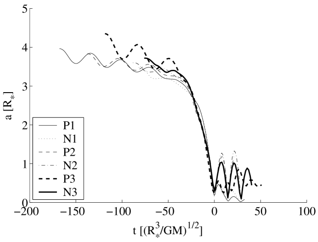
b

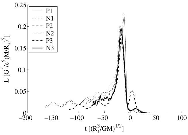
Figure 5: (a) The separation between the centers of mass of the stars (in units of initial radius) as a function of time for all the runs. (b) The gravitational wave luminosity of the system for all the runs.

When comparing a P run to a N run with the same mass, we must take into account that a polytrope that is static in (0+1)PN gravitation is not static in 0PN, Newtonian, gravitation. For the same mass, the Newtonian polytrope has a larger radius. This causes the initial polytrope to grow at the beginning of the N runs as demonstrated in Figure  4. Note that unlike Figure 3a where we show the radii of isolated starts, here we show the radii of the stars in the first timesteps of the coalescence. In order to differentiate between 1PN effects and the effects of these differences in initial conditions, we try to present all results scaled by the appropriate mass and initial radius. For instance, the dynamical orbital instability sets in at $a/R_{*}\approx 3$ (Rasio & Shapiro, 1995) where $a$ is the binary separation. For a N run this is at a larger separation than for a P run with similar mass. This means that the P runs will have to evolve longer with gravitational radiation damping as the only mechanism for decreasing the separation. This behavior can be seen in Figure 5a.

The scaling we use during the rest of the discussion is the following: distance is measured in units of $R_{*}$, luminosity is measured in units of $G^{4}/c^{5}(M/R_{*})^{5}$, rest mass density ($\rho_{*}$) is measured in units of $M/R_{*}^{3}$ and energy in units of the rest mass energy of the star $Mc^{2}$. Time is measured in hydrodynamic time scales $(R_{*}^{3}/GM)^{1/2}$ and is shifted so that for each run the minimal separation occurs at $t=0$. $R_{*}$ is the initial radius of the stars. $M=\int d^{3}x\rho_{*}$ is the conserved mass for each run. We emphasize that in the P runs the conserved mass is not the same as the rest mass.

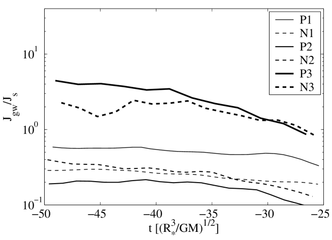
Figure 6: The ratio $J_{\rm gw}/J_{\rm s}$ of angular momentum in the gravitational radiation to angular momentum in stellar spins. The ration is shown up to the time of the dynamical orbital instability. In all runs but N3 and P3 spin-up of the stars is the dominant process for causing the merger.

We define the center of mass of each star to be the center of conserved mass of the particles belonging to the star at the initial time step. Since we use a particle based scheme we can follow particles throughout the simulation and use this definition even after the stars have touched. In Figure 5a we show the separation of the centers of mass of the two stars as a function of time. As can be seen, the runs start in a slightly elliptical orbit which slowly decays. Two distinct processes cause this decay. The first is the conversion of orbital angular momentum into stellar spins $J_{\rm s}$ via gravitational torques. This process is also present in Newtonian gravity. The second process is the emission of gravitational radiation, carrying with it angular momentum $J_{\rm gw}$. This is a 2.5PN process having no Newtonian parallel. The dynamical orbit instability sets in for both the P and N runs as the separation reaches $3R_{*}$, ($t\approx-25$). This causes a rapid plunge, and a merger in about one orbital period. In Figure 6 we show the ratio $J_{\rm gw}/J_{\rm s}$ up to the dynamical instability. In the runs N3 and P3 this ratio is close to unity near $t=-25$. In all other runs it is apparent that the spin-up of the stars plays a more important role than gravitational radiation in causing the merger. The stars touch at $t\approx-15$ (when $a/R_{*}\approx 2$). The minimal separation at $t=0$ is achieved when the cores, which hold most of the mass, have merged. At $t>0$ the centers of mass “bounce”. The bounce is more pronounced for the P2, N2 and N3 runs because of the stiffer EoS used in these runs. In the P3 run however, 1PN gravity is strong enough to counteract this stiffness and the bounce is comparable to that of the P1 and N1 runs.

In Figure 5b we depict the gravitational radiation luminosity (Eq. 4) of the merger. The characteristics of the luminosity peak are similar in all the runs once we allow for the different initial radii of the stars. The P3 run however exhibits a pronounced second peak at $t\approx 5$ at about the same luminosity of the system at the last orbits before the merger. This second peak is absent in all other runs. This distinct feature is a result of the strong 1PN gravity and stiff EoS of the P3 run.

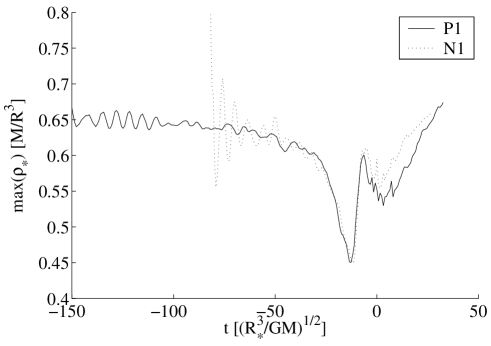
b

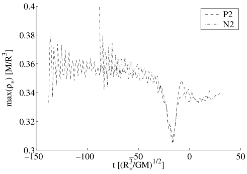
c

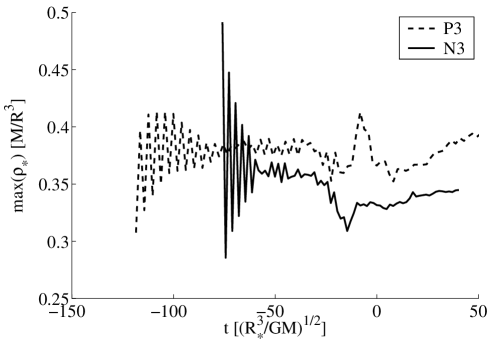
Figure 7: Maximum coordinate rest mass density $\rho_{*}$ in the P and N runs. (a) the P1 and N1 runs. (b) The P2 and N2 runs. (c) The P3 and N3 runs. The maximum drops during the merger and climbs back up afterwards. Notice the distinct rise at $t\approx-5$ in the P3 run

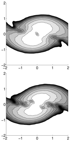
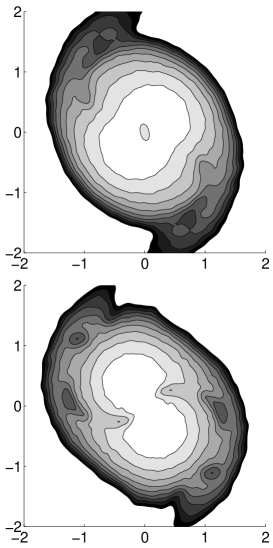
a b c

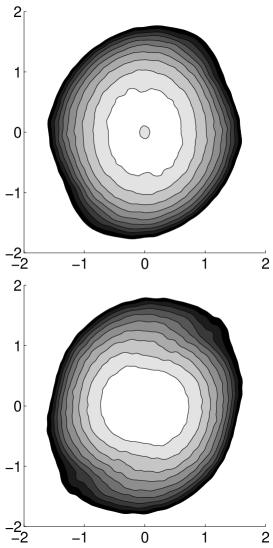
Figure 8: Rest mass density $\rho_{*}$ of the cores of the N3 (top) and P3 (bottom) run. The contours are logarithmic with a spacing of $10^{0.1}$. The length scale is in $R_{*}$. The minimal contour is at 10% of the maximum rest mass density so the spiral arms are not visible in this plot. The cores is shown at times (a) $t\approx-10$. (b) $t\approx 2$. (c) $t\approx 20$.

In order to explain this distinct feature of the P3 run we show in Figure 7 the maximum rest mass density $\rho_{*}$ for all the runs. The P1 and N1 runs exhibit a larger relative density because of their softer EoS. In all the runs we see a dip in the maximum density at the time of the rapid infall caused by the orbital instability. This corresponds to the stars shedding each other’s mass as they move closer together. This stage ends at $t\approx-15$, when the stars touch, and is followed by a fast rise up to $t\approx-7$. The difference between the N2 and N3 runs and the N1 run can be attributed to the softer EoS of the latter while the difference between them and their respective P runs is due to the stronger gravitational attraction in the P runs. The maximum density in the N2 and N3 runs does not have the peak at $t\approx-7$ which is evident in all other runs, most distinctly in the P3 run where it rises to about 10% more than it’s final value. It is in this run where the stiff EoS and the strong 1PN gravity combine to induce a large compression of the cores which delays their final merger into a single axisymmetric central object. This delay turns the merger into a two part process and produces the second peak in the luminosity at $t\approx 3$. This can be seen in Figure 8 where we compare the cores of the P3 and N3 runs at $t\approx-10,2,20$. $t\approx-10$, is just after the first peak in the luminosity. We see the in the N3 run the cores have almost merged. At $t\approx 2$ the cores in the N3 run have merged and formed an almost axisymmetric object which emits very little gravitational radiation, on the other hand the P3 cores are still almost separate and certainly far from axial symmetry. At $t\approx 20$ the cores of the P3 run have already merged completely and emit little gravitational radiation as well.

In this context it is interesting to note Ruffert et al. (1997) where there is a comparison of the gravitational wave luminosity produced by different numerical schemes. SPH is found to inhibit the second peak in the gravitational wave luminosity possibly because of the numerical viscosity. Using other numerical schemes the second peak in the luminosity is about one half the height of the first peak. This raises the possibility that 1PN terms, may in reality have an even more prominent effect on the luminosity.

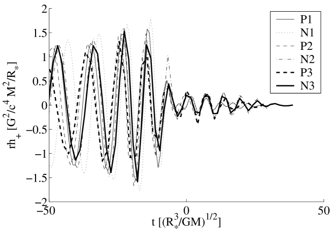
b

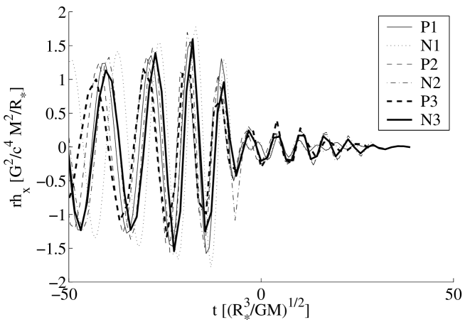
Figure 9: The gravitational radiation waveforms for an observer situated along the rotation axis (z axis) in geometrical units as a function of time. (a) The $+$ polarization. (b) The $\times$ polarization

The actual gravitational waveforms emitted by the systems are shown in Figure 9. Here we see a difference in the period of the waveforms between the P and N runs corresponding to a different orbital period before the actual merger. During and after the merger there is no qualitative difference between the waveforms.

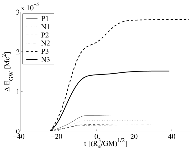
Figure 10: The energy emitted in gravitational waves for the P and N runs. The calculation was started at $t=-25$ when the runs had about the same relative separation.

In Figure 10 we compare the total energy emitted by gravitational waves. We start the comparison at $t=-25$ when all runs have roughly the same relative separation, before the stars touch. When comparing the similar mass runs P1, N1, P2, and N2 we see that a softer EoS implies more energy emitted in gravitational waves, while the more massive runs P3 and N3 emit an order of magnitude more energy as compared to run P2 and N2 which have a similar EoS. The P3 run emits almost twice the energy of the N3 run. We note that in this figure the axis scaling is different from Figure 5b e.g. run P3 and N3 have almost similar $L$ in Figure  5b, but since it is scaled by $R_{*}^{5}$ the actual P3 luminosity is a factor of $\approx 2$ higher than the N3 luminosity

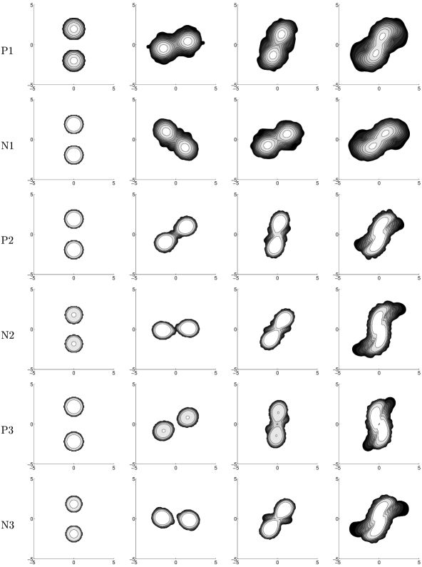
Figure 11: Coordinate rest mass density contours for the runs. Time increases to the right. The length scale is in $R_{*}$. The contours are taken at the initial time step, $t=-40$, $t=-25$ (beginning of dynamical instability) and $t=-15$ ($a=2R_{*}$). The rest mass density is in units of $M/R_{*}^{3}$ and the contours are logarithmic with a spacing of $2.3$ starting at 1

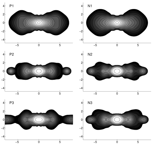
Figure 13: Coordinate rest mass density ($\rho_{*}$) in units of $(M/R_{*}^{3})$ for the final configuration ($t=20$) on the $x-z$ plane. The contours are logarithmic with a spacing of $2.1$ starting at 1. The length scale is in $R_{*}$

We now turn to look at the morphological differences between the runs. In Figures 11 and  12 we show the contours of coordinate rest mass density on the orbital ($x-y$) plane at various times. The difference due to the different EoSs is the most striking. The P1 and N1 runs lead to a final configuration with almost non-existent spiral arms, which are very prominent in the P2, N2, P3, and N3 runs. There is almost no difference between the N1 and P1 results, while we see that N2 and N3 result in longer spiral arms than P2 and P3 respectively. This is most prominent in the difference between N3 and P3. The central object at $t=20$ is approximately the same size in all the runs and is axisymmetric. For a closer look at this central object we show contours of the rest mass density at t=20 in the $x-z$ plane (Fig. 13). In all the runs we see a central core, with a density above $0.1M/R_{*}^{3}$ and which has an equatorial radius of approximately $1.5R_{*}$. The polar radius is smaller in the N1 and P1 runs than in the P2, N2, P3, and N3 runs. Surrounding this core is a halo with a radius of about $5R_{*}$. The halo is extended vertically in the N1 and P1 runs up to a distance of $3R_{*}$, while in the P2, N2, N3, and P3 runs it has a height of only $2R_{*}$. The P3 run resulted in the most compact object, as could be expected. In all runs, there is a funnel, a zone of low density, around the axis of rotation.

Finally, we calculate how much mass can escape the system. We do this by counting all the particles in the final configuration which are at a distance greater than $6R_{*}$ from the origin and which have positive total Newtonian energy. The total Newtonian energy of a particle is $E_{\rm Newt}=\frac{1}{2}mv^{2}+m\varepsilon-mU_{*}$ with $\varepsilon$ the specific internal energy and $U_{*}$ (Eq. A8) the Newtonian gravitational potential. Particles which are closer than $6R_{*}$ will surely interact with other particles before exiting the system and so their energy won’t be conserved. For particles further than this, the gravitational potential $U_{*}$ is of the order of 0.01 and the velocity is of the order of 0.1c which ensures that the Newtonian energy will be conserved. Only in run N2, P2 and N3 have any particles escaped, as shown in Table 1. The N2 has the highest escaped mass followed by N3. For the other runs we are only able to give upper bounds on the escaped mass by using the mass of the lightest particles in the run. It’s these minimal mass particles which escape since they are located at the surface of the stars in the initial conditions. We note that escaped mass is also given in Rosswog et al. (1999). However a comparison between our results is impossible since we use different initial conditions and EoSs.

5 Summary

We have introduced here a PN adaptation of the Tree+SPH algorithm. This adaptation is made possible by the BDS formalism which recasts the (0+1+2.5)PN equations of gravity and hydrodynamics in a form resembling the Newtonian equations. We have tested various aspects of our code by comparing the numerical results with known analytical solutions of relativistic problems. The (0+1)PN hydrodynamic part had been tested using a relativistic shock tube; the 2.5PN gravitational radiation reaction terms were tested using two point masses in orbit and the 1PN gravitation+hydrodynamic terms were tested using a spherical static OV polytrope. The code passes all these tests with the expected accuracy.

Using this code we have investigated the 1PN effects on BNS coalescence. We compare runs with identical initial conditions but different physics. In the N runs, we use only the (0+2.5)PN terms, in the P runs we include also the 1PN terms. In both runs we keep the 2.5PN gravitational radiation terms. These terms lead to a slow decreases of the orbital separation until a critical separations is reached. At this point a dynamical instability sets in and the stars merge within one orbital period. We use polytropes with a mass of less than $M_{\odot}$ and a radius of about 30Km for the runs. These are not typical NS parameters but the (0+1+2.5)PN approximation in the BDS formalism is valid only when the 1PN terms are small compared to the 0PN terms and this set an upper limit to the compactness of the stars. Therefore, Our results do not describe typical BNS coalescence, but rather the effect of the 1PN terms on this process.

Our results show that when going up to higher masses and thus to more relativistic conditions, there appears a prominent peak in the maximum rest mass density just before the cores merge in the P3 run. This peak is absent in the N3 run. This peak in rest mass density could mean a that the probability of the coalesced object collapsing into a black hole is larger than that estimated by Newtonian codes. Also, we see that the energy emitted in gravitational waves is almost twice as large in the P3 run as compared with the N3 run. This difference is also seen in the profile of the gravitational wave luminosity of the system. This result supports the suggested idea to use the gravitational wave signal as a probe on the details of the merger process. Our simulations show that the absence of a prominent second peak in the luminosity indicates a soft EoS.

Appendix A BDS Equations

We use the Lagrangian formulation of the BDS equations (Blanchet et al., 1990). First we define some auxiliary quantities

$$\alpha = 2U_{*}-\gamma_{*}\left({\textstyle\frac{1}{2}}{\bf w}^{2}+3U_{*}\right),$$ (A1)

$$\beta = {\textstyle\frac{1}{2}}{\bf w}^{2}+3U_{*}+\varepsilon_{*}+\frac{p_{*}}{\rho_{*}},$$ (A2)

$$\delta = {\textstyle\frac{3}{2}}{\bf w}^{2}+\varepsilon_{*}+3\frac{p_{*}}{\rho_{*}}-U_{*},$$ (A3)

$$A_{i} = 4U_{i}+{\textstyle\frac{1}{2}}C_{i}-{\textstyle\frac{1}{2}}x^{i}\partial_{s}U_{s},$$ (A4)

$$U_{5} = {\textstyle\frac{3}{2}}\left(R-Q^{[3]}_{ij}x^{i}\partial_{j}U_{*}\right),$$ (A5)

$$P_{ij} = 2\int d^{3}x\,\rho_{*}\left(3w_{i}\partial_{j}U_{*}-2\frac{w_{i}}{\rho_{*}}\partial_{j}p_{*}+x^{i}w_{s}\partial_{sj}U_{*}-x^{i}\partial_{sj}U_{s}\right),$$ (A6)

$$Q^{[3]}_{ij} = {\textstyle\frac{1}{2}}\left(P_{ij}+P_{ji}\right)-{\textstyle\frac{1}{3}}\delta_{ij}P_{ss},$$ (A7)

where $p_{*}=p(e_{*},\rho_{*})$ is the pressure, $\gamma_{*}=\partial\log p_{*}/\partial\log\rho_{*}$ is the adiabatic index and ${\bf w}^{2}=w_{i}w_{i}$. Using these quantities we solve the following Poisson equations

$$\triangle U_{*} = -4\pi G\rho_{*},$$ (A8)

$$\triangle U_{i} = -4\pi G\rho_{*}w_{i},$$ (A9)

$$\triangle C_{i} = -4\pi Gx^{i}\partial_{s}\left(\rho_{*}w_{s}\right),$$ (A10)

$$\triangle U_{2} = -4\pi G\rho_{*}\delta,$$ (A11)

$$\triangle R = -4\pi GQ^{[3]}_{ij}x^{i}\partial_{j}\rho_{*}.$$ (A12)

The forces and the velocity are defined next

$$v^{i} = w_{i}-\frac{1}{c^{2}}\beta w_{i}+\frac{1}{c^{2}}A_{i}+\frac{4}{5}\frac{G}{c^{5}}w_{s}Q^{[3]}_{is},$$ (A13)

$$F^{\mbox{\scriptsize press}}_{i} = -\frac{1}{\rho_{*}}\partial_{i}\left[\left(1+\frac{\alpha}{c^{2}}\right)p_{*}\right],$$ (A14)

$$F^{\mbox{\scriptsize 1PN}}_{i} = \left(1+\frac{\delta}{c^{2}}\right)\partial_{i}U_{*}+\frac{1}{c^{2}}\partial_{i}U_{2}-\frac{1}{c^{2}}w_{s}\partial_{i}A_{s},$$ (A15)

$$F^{\mbox{\scriptsize reac}}_{i} = \frac{G}{c^{5}}\partial_{i}U_{5}.$$ (A16)

We are now in position to advance the system in time using the evolution equations

$$\dot{\rho_{*}} = -\rho_{*}\partial_{i}v^{i},$$ (A17)

$$\dot{\varepsilon_{*}} = -\frac{p_{*}}{\rho_{*}}\partial_{i}v^{i},$$ (A18)

$$\dot{x^{i}} = v^{i},$$ (A19)

$$\dot{w_{i}} = F^{\mbox{\scriptsize press}}_{i}+F^{\mbox{\scriptsize 1PN}}_{i}+F^{\mbox{\scriptsize reac}}_{i},$$ (A20)

where the dot represents the Lagrangian time derivative $\dot{a}\equiv\partial_{t}a+v^{i}\partial_{i}a$.

Appendix B Adapting the Barnes-Hut tree to solve general Poisson equations

The Barnes-Hut tree is a method for calculating the gravitational force between $N$ particles in $N\log N$ operations. The force on a given particle is calculated by summing the forces from individual particles if they are close, and by using a multipole approximation for far away clusters of particles. A cluster is considered far away if $d/l<\theta$ where $d$ is the clusters size, $l$ is it’s distance and $\theta$ is an external parameter governing the degree of approximation of the method. The tree itself is a data structure specially adapted for efficient clustering of particles and calculations of the multipole moments. In practice the multipole approximation is accurate enough to be stopped at the quadrupole term.

Although it was originally invented for the calculation of gravitational forces, the Barnes-Hut tree can solve any compact supported Poisson equation with little modification. Given the multipole moments of the source of the equation, the potential and its derivatives can be calculated in an analogous way to the calculation of the gravitational potential and force in the following way:

Given a compact source $\eta$ and the masses and densities of each particle, we will solve the Poisson equation

$$\triangle U=-4\pi\eta.$$ (B1)

The first three multipole moments of a cluster of particles are

$$M^{\eta} = \sum_{p}\frac{m_{p}}{\rho_{p}}\eta_{p},$$ (B2)

$$D^{\eta}_{i} = \sum_{p}\frac{m_{p}}{\rho_{p}}\eta_{p}x^{i}_{p},$$ (B3)

$$Q^{\eta}_{ij} = \sum_{p}\frac{m_{p}}{\rho_{p}}\eta_{p}\left(x^{i}_{p}x^{j}_{p}-{\textstyle\frac{1}{3}}\delta_{ij}x^{n}_{p}x^{n}_{p}\right),$$ (B4)

where the index $p$ runs over the cluster particles, $m_{p}$ and $\rho_{p}$ are the particle mass and density (so that $m_{p}/\rho_{p}\approx V_{p}$ the particle volume) $\eta_{p}$ is the value of $\eta$ on the particle and $x^{i}_{p}$ is the $i$-th component of the particle coordinate.

Using these moments the cluster’s potential and it’s derivatives can be calculated as follows:

$$U^{\eta} = \frac{M^{\eta}}{r}-\frac{D^{\eta}_{i}x_{i}}{r^{3}}+\frac{1}{2}\frac{x_{i}x_{j}Q^{\eta}_{ij}}{r^{5}}$$ (B5)

$$\partial_{k}U^{\eta} = -\frac{M^{\eta}}{r^{3}}x_{k}$$

$$-\frac{1}{r^{3}}D^{\eta}_{k}+3\frac{D^{\eta}_{i}x_{i}}{r^{5}}x_{k}$$

$$+\frac{x_{j}Q^{\eta}_{jk}}{r^{5}}-\frac{5}{2}\frac{x_{i}x_{j}Q^{\eta}_{ij}}{r^{7}}x_{k}$$

$$\partial_{lk}U^{\eta} = -\frac{M^{\eta}}{r^{3}}\delta_{lk}+3\frac{M^{\eta}}{r^{5}}x_{k}x_{l}$$ (B6)

$$+3\frac{1}{r^{5}}\left(D^{\eta}_{k}x_{l}+D^{\eta}_{l}x_{k}-D^{\eta}_{i}x_{i}\delta_{lk}\right)+15\frac{D^{\eta}_{i}x_{i}}{r^{7}}x_{k}x_{l}$$

$$+\frac{Q^{\eta}_{kl}}{r^{5}}-10\frac{x_{i}x_{l}Q^{\eta}_{ik}}{r^{7}}-\frac{5}{2}\frac{x_{i}x_{j}Q^{\eta}_{ij}}{r^{7}}\delta_{kl}+\frac{35}{2}\frac{x_{i}x_{j}Q^{\eta}_{ij}}{r^{9}}h_{k}x_{l}$$

where $r$ is the distance to the cluster, $\delta_{ij}$ is the Kronecker delta and a double index is summed over.

a

a

a

a

a

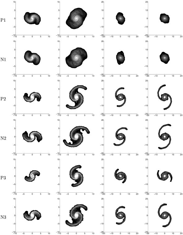
Figure 12: Coordinate rest mass density contours for the runs. Time increases to the right. The length scale is in $R_{*}$. The contours are taken at $t=-7$ (peak in Fig 7c), $t=0$ (minimal separation), $t=10$ and $t=20$. The rest mass density is in units of $M/R_{*}^{3}$ and the contours are logarithmic with a spacing of $2.3$ starting at 1

References

- Barish (1998) Barish, B. C. 1998, in New Worlds in Astroparticle Physics, Proceedings of the International Workshop, held 8-10 September, 1996, Faro, Portugal. Edited by Ana M. Mourao, Mario Pimenta, Robertus Potting, and Peter Sonderegger. World Scientific Publishers, 1998., p.391, 391+
- Barnes & Hut (1986) Barnes, J. & Hut, P. 1986, Nature, 324, 446
- Baumgarte et al. (1998) Baumgarte, T. W., Cook, G. B., Scheel, M. A., Shapiro, S. L., & Teukolsky, S. A. 1998, Phys. Rev. D, 57, 7299, gr-qc/9709026
- Benz (1990) Benz, W. 1990, in The Numerical Modeling of Nonlinear Stellar Pulsations: Problems and Prospects, ed. J. R. Buchelr (Dordrecht: Kluwer), 269–288
- Benz et al. (1990) Benz, W., Cameron, A. G. W., Press, W. H., & Bowers, R. L. 1990, ApJ, 348, 647
- Blanchet et al. (1990) Blanchet, L., Damour, T., & Schaefer, G. 1990, MNRAS, 242, 289
- Davies et al. (1994) Davies, M. B., Benz, W., Piran, T., & Thielemann, F. K. 1994, ApJ, 431, 742
- Davies et al. (1993) Davies, M. B., Ruffert, M., Benz, W., & Muller, E. 1993, A&A, 272, 430+
- Fidecaro & Collaboration (1997) Fidecaro, F. & Collaboration, V. 1997, in General Relativity and Gravitational Physics; Proceedings of the 12th Italian Conference, edited by M. Bassan, V. Ferrari, M. Francaviglia, F. Fucito, and I. Modena. World Scientific Press, 1997., p.163, 163+
- Flanagan (1999) Flanagan, E. E. 1999, Phys. Rev. Lett., 82, 1354
- Font et al. (1998) Font, J. A., M., M., Suen, W., & M., T. 2000, Phys. Rev. D, 61, 044011
- Hawley et al. (1984) Hawley, J. F., Wilson, J. R., & Smarr, L. L. 1984, ApJ, 277, 296
- Hernquist & Katz (1989) Hernquist, L. & Katz, N. 1989, ApJS, 70, 419
- Hough et al. (1996) Hough, J., Newton, G. P., Robertson, N. A., Ward, H., Campbell, A. M., Logan, J. E., Robertson, D. I., Strain, K. A., Danzmann, K., Lück, H., Rüdiger, A., Schilling, R., Schrempel, M., Winkler, W., Bennett, J. R. J., Kose, V., Kühne, M., Scultz, B. F., Nicholson, D., Shuttleworth, J., Welling, H., Aufmuth, P., Rinkleff, R., Tünnermann, A., & Willke, B. 1996, in Proceedings of the Seventh Marcel Grossman Meeting on recent developments in theoretical and experimental general relativity, gravitation, and relativistic field theories. Proceedings of the Meeting held at Stanford University, 24-30 July 1994. Edited by Robert T. Jantzen, G. Mac Keiser, and Remo Ruffini, River Edge, New Jersey: World Scientific, 1996., p.1352, 1352+
- Kheyfets et al. (1990) Kheyfets, A., Miller, W. A., & Zurek, W. H. 1990, Phys. Rev. D, 41, 451
- Kley & Schäfer (1999) Kley, W. & Schäfer, G. 1999, Phys. Rev. D, 60, 027501
- Kozai & Tama-300 Collaboration (1999) Kozai, Y. & Tama-300 Collaboration. 1999, in 4th East Asian Meeting on Astronomy (4th EAMA) - Observational Astrophysics in Asia and its Future (Yunnan Observatory, Chinese Academy of Sciences)
- Laguna et al. (1993) Laguna, P., Miller, W. A., & Zurek, W. H. 1993, ApJ, 404, 678
- Lombardi et al. (1999) Lombardi, J. C., Sills, A., Rasio, F. A., & Shapiro, S. L. 1999, J. Comp. Phys., 152, 687
- Mathews & Wilson (1997) Mathews, G. J. & Wilson, J. R. 1997, ApJ, 482, 929+
- McKee & Colgate (1973) McKee, C. R. & Colgate, S. A. 1973, ApJ, 181, 903
- Monaghan (1992) Monaghan, J. J. 1992, ARA&A, 30, 543
- Oohara & Nakamura (1997) Oohara, K. & Nakamura, T. 1997, in Relativistic Gravitation and Gravitational Radiation; Proceedings of the Les Houches School of Physics 26 Sept - 6 Oct, edited by J.A. March and J.P. Lasota, Cambridge University Press, 1997., p.309, 309+, astro-ph/9606179
- Rasio & Shapiro (1991a) Rasio, F. A. & Shapiro, S. L. 1991a, ApJ, 377, 559
- Rasio & Shapiro (1991b) —. 1991b, ApJ, 401, 226
- Rasio & Shapiro (1995) —. 1995, ApJ, 438, 887
- Rosswog et al. (1999) Rosswog, S., Liebendörfer, M., Thielemann, F. K., Davies, M. B., Benz, W., & Piran, T. 1999, A&A, 341, 499
- Ruffert & Janka (1998) Ruffert, M. & Janka, H. T. 1998, A&A, 338, 535
- Ruffert et al. (1997) Ruffert, M., Rampp, M., & Janka, H.-T. 1997, A&A, 321, 991
- Shapiro & Teukolsky (1983) Shapiro, S. L. & Teukolsky, S. A. 1983, Black holes. white dwarfs, and neutron stars (Wiley-Interscience)
- Shibata (1997) Shibata, M. 1997, Phys. Rev. D, 55, 6019
- Shibata (1998) —. 1998, Phys. Rev. D, 58, 024012, gr-qc/9803085
- Shibata et al. (1998) Shibata, M., Baumgarte, T. W., & Shapiro, S. L. 1998, Phys. Rev. D, 58, 023002, gr-qc/9805026
- Shibata et al. (1997) Shibata, M., Oohara, K., & Nakamura, T. 1997, Prog. Theor. Phys., 98, 1081
- Siegler & Riffert (1999) Siegler, S. & Riffert, H. 2000, ApJ, 531, 1053
- Taub (1948) Taub, A. H. 1948, Phys. Rev., 74, 328
- Taylor (1994) Taylor, J. H. 1994, Rev. Mod. Phys., 66, 711
- Wang & Swesty (1997) Wang, E. Y. M. & Swesty, F. D. 1997, American Astronomical Society Meeting, 190, 3803+
a
b
c
a
b
a
b
a
b
c
a b
b c
c
a
b