N-body simulations of globular cluster tides

Abstract

We present N-body simulations of globular clusters, in orbits around the Galaxy, in order to study quantitatively and geometrically the tidal effects they encounter. The clusters are modelised with multi-mass King-Michie models (Michie 1963), including mass segregation at initial conditions. The Galaxy is modelled as realistic as possible, with three components: bulge, disk and dark halo. The main finding is that there exist two giant tidal tails around the globuler cluster in permanence along its orbit, whatever this orbit. The length of these tails is of the order of 5 tidal radii, or greater. The escaped stars are distributed radially as a power law in density, with a slope of –4. The tails present substructures, or clumps, that are the relics of the strongest shocks. Due to the compressive disk-shocking, the clusters display a prolate shape which major axis is precessing around the z axis. The tails are preferentially formed by the lowest mass stars, as expected, so that the tidal truncation increases mass segregation. Internal rotation of the cluster increases the mass loss. The flattening of dark matter cannot influence significantly the dynamics of the clusters. The orientation and the strength of the tidal tails are signatures of the last disk crossing, so that observed tidal tails can constrain strongly the cluster orbit and the galactic model (vertical scale of the disc).

1 Introduction

Globular clusters are fascinating systems, since contrary to their apparent geometrical simplicity, they are the sites of many complex physical phenomena. The two-body relaxation time is on average of the order of 10⁹ yr, shorter than their life-time, so that the relaxation is very efficient especially in the core, where the memory of the cluster’s initial conditions is expected to be washed out (see the review by Spitzer 1987). The result of this relaxation is a slow collapse of the core, while the less bound stars in the envelope evaporate. Moreover, the relaxation tends to establish equipartition of energy, and mass segregation, so that the low-mass stars are preferentially expelled into the envelope. Mass loss due to stellar evolution is no longer significant for the old clusters in our Galaxy, but internal dynamical evolution alone could destroy a large fraction of the population (Hénon 1961). In terms of the half-mass relaxation time t_rh, the collapse of the core occurs in $\sim$ 15 t_rh, while total evaporation occurs in $\sim$ 100 t_rh. The core collapse is however unspectacular, involving less than 1% of the stars; it can be reversed, and gravothermal oscillations can happen, according to the amount of heating provided by binaries (Makino 1996, Kim et al. 1998).

External perturbations can considerably accelerate the evolution of globular clusters: compressive shocks at the crossing of the galactic plane, tidal interaction with the bulge, or the dark matter halo. These external perturbations do much more than a tidal limitation of a cluster in a circular orbit, corresponding to a time-independent external potential; they are also cause of tidal stripping and heating of the cluster (Allen & Richstone 1988). Paradoxically, they also accelerate the core collapse (Spitzer & Chevalier 1973). Much effort has been devoted to quantify the dynamical evolution of clusters, since it is crucial to be able to deduce their initial number and distribution and to go back to the Galaxy formation. This has been done with the Fokker-Planck method, orbit-averaging the relaxation effects, and estimating the tidal shocks through impulse approximations (Chernoff et al. 1986, Aguilar et al. 1988). It was already concluded that the number of remaining globular clusters now is a small fraction of those formed initially (Aguilar et al. 1988). The majority of them were destroyed in the early Galaxy evolution, through violent dynamical interactions. Kundić & Ostriker (1995) and Gnedin & Ostriker (1997) have revised these estimates, showing that the second-order tidal shocking ($<\Delta E^{2}>$) is even more important than the first order ($<\Delta E>$); the corresponding shock-induced relaxation could dominate the two-body relaxation. It ensues that about 75% of all present globular clusters will be destroyed in the next Hubble time, which is compatible with observational estimates (Hut & Djorgovski 1992). Since already the more fragile are missing today, and in particular there is a depletion of clusters orbiting within the central 3 kpc of the galaxy, it is likely that the initial cluster population was more than an order of magnitude more numerous than today.

Many uncertainties remain when trying to quantify the present mass loss of globular clusters. The effect of irregularitites in the disk potential on the clusters evolution have been studied: Giant Molecular Clouds (Chernoff et al. 1986), spiral arms and bars (Ostriker et al. 1989, Long et al. 1992) are found to be only a secondary effect in the destruction of the clusters, the crossing of a thin plane being the dominant factor (and also the bulge crossing in the inner parts, Nordquist et al. 1999). Multi-mass models undergo more rapid evolution than single-mass models (Lee & Goodman 1995): the rate of mass loss can be doubled per half-mass relaxation time. Internal rotation of clusters, that was more important in the past, might be a significant factor, too.

Recently Grillmair et al. (1995) observed the outer parts of 12 Galactic globular clusters, using deep two color star counts. They discovered huge tidal tails, consisting of stars escaping the clusters, that can help to quantify the mass loss, and to bring some constraints on the cluster orbits. We have also carried out such a photometric study on 20 Galactic clusters (Leon et al. 1999), and report about the characteristics of the tidal tails, once the main observational biases are taken into account (extinction, galaxy clusters, etc…). In the present work, we try to reproduce the observations, in order to better quantify the effect of external perturbations from the Galaxy on clusters, with mass segregation and rotation included. In particular we want to identify the fate of escaped stars, and relate the tidal tails morphology to the cluster orbits. In Section 2, we first describe the methods used, together with the models adopted for the globular clusters and the Galaxy potential, and describe the results of the simulations in Section 3. Section 4 summarizes the results.

2 Numerical methods

2.1 Overwiew

One of the most important problem in simulating the dynamical evolution of globular clusters, is the wide range of time-scales involved. Two kinds of methods have been used: either an N-body integration with various algorithms, following the internal stellar orbits, which have a dynamical time of the order 1 Myr; but the method is expensive since the total simulation must be carried out over Gyrs; also the two-body relaxation might be over- or under-estimated, according to the number of particles used and the softening. Alternatively, the Fokker-Planck or Monte-Carlo methods are used, with orbit-averaging and use of diffusion coefficients to take into account the two-body relaxation effects. But then external gravitational perturbations cannot be evaluated exactly, and approximations are used, as adiabatic invariants, impulse approximation, steady potentials, etc…

Weinberg (1994a,b,c) has shown that the adiabatic approximation, consisting in neglecting the effect of perturbations slow enough with respect to the internal stellar periods, is generally not valid for stellar systems, that are heated by slow perturbations. Widely used is also the impulse approximation, that assumes a very rapid perturbation (or shock) with respect to internal motions; however, this is only a crude estimate (Johnston et al. 1999). Adiabatic corrections are required, and are rather critical, since they can multiply the cluster destruction time by a factor two (Gnedin et al. 1998, 1999, Gnedin & Ostriker 1999).

Oh et al. (1992a,b, 1995) developped an hybrid method, using the Fokker-Planck equations for the cluster center, monitoring the effects of two-body relaxation, and a three-body integration for the envelope. They have been able to follow escaped particles up to 10 initial limiting radii after 20 orbits around the galaxy. Recently Johnston et al. (1999) used the SCF (self-consistent field) method developped by Hernquist & Ostriker (1992), allowing to simulate clusters with the actual number of stars (of the order of 10⁶). The Poisson noise is therefore exactly natural, however the two-body relaxation is under-estimated, except in rare cases when a Fokker-Planck diffusion scheme is added to the N-body code. For a long time, Fokker-Planck calculations appeared to yield much lower lifetimes for clusters in the Galaxy, compared to N-body simulations. Both methods are now converging (Takahashi & Portegies Zwart 1999).

Our aim here is to determine and quantify the tidal effects of the Galaxy on a globular cluster along one orbit, on a time-scale of the order of t_rh; we do not focus on long-term effects, and do not follow the cluster until its destruction. The two-body relaxation is only approximated, and we do not take into account dynamical friction, which occurs on very long time-scale and for very massive clusters only. We assume the globular cluster old enough so that the effects of stellar evolution are negligible. We however take into account the mass segregation inside the cluster, since it can affect the tidal tail behaviour or the mass loss, most of the small stellar masses being confined in the outer parts. We will focus on the characteristics of the tidal tails, their amplitude, and 3D shapes, in order to compare with observations, and therefore to put constraints on the globular clusters orbits and mass loss.

2.2 Algorithm

The N-body code used is an FFT algorithm, using the method of James (1977) to avoid the periodic images. This method finds correction charges on the 2D boundary surfaces, which, once convolved with the Green function, cancel out the effect of images. It increases considerably the efficiency of the FFT method, especially in 3D, since it avoids to multiply by 8 the volume where the FFT is computed. We used a 128³ grid with N=1.5 10⁵ particles, which required 2.7s of CPU per time step on a Cray-C94. The Green function used is the g₂ function from James (1977), so that the deviation from Newtonian law is of the order of $R^{-5}$, at large distance $R$; the resulting softening parameter is of the order of the grid size, i.e. 1pc. The units used in the simulations are pc, km/s, Myr, and G=1 (the corresponding unit of mass is then 2.32 10² M_⊙).

2.3 Cluster model

We used several initial cluster models, built from Michie-King multi-mass distributions. We divide the particules in 10 mass bins, distributed logarithmically. The stellar masses in old globular clusters range from 0.12 to 1.2 M_⊙ essentially, so we simulate a mass spectrum over one decade. Although the mass turn-over is around 0.8 M_⊙ for such old star populations, one should also take into account the remnants of massive stars that contribute to replenish the high-mass end. We adopt the Salpeter mass function for the spectrum, i.e. $dN/dm\propto m^{-2.35}$. With such a spectrum, which represents quite nicely the observations (Richer et al. 1991), the total number of stars is of the order of 1.2 10⁶ for a cluster mass of 3 10⁵ M_⊙ (or an average mass of 0.24 M_⊙). Since we use a constant total number of particles of 1.6 10⁵ for all our models, whatever their total mass, there will not be exact correpondence between particles and stars, but particles are statistically representative of the stars. Therefore, we ignore the possible depletion of stars at both ends, to only consider power-law mass spectra within the two mass limits.

To find the distribution function for each mass class, we integrate the Poisson equation iteratively, with the method described by da Costa & Freeman (1976). The starting solution for each mass is the single-mass distribution function

$$f(\epsilon)=\rho_{0}(2\pi\sigma_{0}^{2})^{-3/2}(e^{\epsilon/\sigma_{0}^{2}}-1)\quad\quad\epsilon>0$$

where $\epsilon=\Psi-\frac{1}{2}v^{2}$ and $\Psi(r)=-\Phi(r)+\Phi(r_{t})$, $\Phi$ being the gravitational potential, $\sigma_{0}$ the central velocity dispersion and $r_{t}$ the tidal radius. Each model is determined by three initial parameters, the King core radius r₀, the depth of the potential $W_{0}$, and the central velocity dispersion $\sigma_{0}$. The central density $\rho_{0}$ is then derived through the relation:

$$r_{0}^{2}={{9\sigma_{0}^{2}}\over{4\pi G\rho_{0}}}$$

The velocity dispersions for each mass class is determined through equipartition of energy. Only a few iterations are required for a relative accuracy of 10^-3, and the resulting solution gives the total mass, the limiting radius, and the final radial density distributions plotted in Fig. 1. The degree of mass segregation can be estimated from Fig. 3.

Figure 1: Volumic (upper panel) and surface (lower panel) radial total density distributions for five of our globular cluster models. The dotted lines correspond to models m5 and m6 (see Table 1.)

2.4 Rotation

Rotation is at present very weak in globular clusters. It has been measured convincingly only in the brightest cluster, $\omega$ Centauri (Meylan & Mayor 1986, Merritt et al. 1997), where the rotation is almost solid-body until about 15% of the tidal radius, and then falls off quickly. It seems that rotation is correlated with flattening (Meylan & Mayor 1986, Davoust & Prugniel 1990), which is compatible with the result of ”isotropic oblate rotator” found in $\omega$ Cen. The average observed flattening is $b/a$ = 0.9, but an important fraction of the clusters have axis ratios smaller than that, between 0.8-0.9. Since two-body relaxation is efficient in the core, and erases all possible primordial anisotropy, the flattening of globular clusters is likely due to rotation, contrary to elliptical galaxies.

The influence of rotation on the dynamical evolution of clusters has been investigated by Lagoute & Longaretti (1996) and Longaretti & Lagoute (1997a,b). The rate of evaporation is increased significantly (up to a factor of 3 to 4) per relaxation time, although the latter is somewhat lengthened. Stellar escape reduces the amount of rotation and flattening, a result compatible with the observation of decrease of flattening with age (Frenk & Fall 1982). Globular clusters with shorter relaxation time are also rounder (Davoust & Prugniel 1990), which supports the loss of rotation with relaxation.

Gravitational shocks at disk crossing produces an apparent flattening, mainly parallel to the galactic plane. It has long been argued that the observed flattening could not be due to the galactic tidal field, because its direction is not aligned with the galactic center (see Lagoute & Longaretti 1996); but this is not the expectation for compressive shocks. Also, it is possible that tidal interactions increase the rotation of the clusters. These effects are investigated below.

To incorporate rotation in the initial cluster models, a distribution function $f(\epsilon,L_{z})$ should be chosen, corresponding to a flattened density distribution $\rho(r,z)$; however, only a few studies have developped in this domain (cf Wilson 1975, Dejonghe 1986), and no analytic function has been found corresponding to the likely rotation curve of clusters. The density is only a function of the even distribution $f_{+}=0.5(f(\epsilon,L_{z})+f(\epsilon,-L_{z}))$, since of course the sense of rotation does not influence the spatial density, so that for a given flattened cluster, an infinite distribution functions could be chosen, the odd function $f_{-}=0.5(f(\epsilon,L_{z})-f(\epsilon,-L_{z}))$ indicating the rotational velocity. Since the rotation is only a very weak effect, we have selected another scheme to introduce it. From a non-rotating cluster model, we select a certain fraction of the particles, and reverse their sign of velocity ( ${\bf v}$ in $-{\bf v}$) if their projected angular momentum $L_{z}$ is not positive. This process consists in introducing and $L_{z}$-odd part $f_{-}$ in the initial distribution. This algorithm allows to control the amount of rotation by the fraction selected, as a function of radius. In practice, selecting particles whatever their radius already results in a rotation curve very compatible with that observer for $\omega$ Cen by Merritt et al. (1997). The cluster is not exactly in equilibrium at start, but is left to violently relax (varying potential) during a few crossing times ($\sim$ 10 Myr), and reaches quickly a flattened relaxed state, with flattening of the order $b/a\approx 0.9-0.95$. The resulting rotation profile is displayed in Fig. 2.

Figure 2: Rotational profile of the cluster model m2 (dash-line), velocity dispersion profile (dash-dot) and projected density profile (full line), as would be observed in projection perpendicular to the rotation axis.

Figure 3: Radial density law for the 10 mass bins for some of the globular cluster models. The highest curve corresponds to low masses, they are all normalised to it. For the case m6, owing to the higher concentration, the lower mass stars are less numerous in the center.

Table 1 displays the principal parameters of the cluster models: the mass, the concentration c = log ($r_{t}/r_{c}$), the core radius $r_{c}$ where the surface density is halved, the half-mass radius $r_{h}$, the tidal radius $r_{t}$ which is here the limiting radius of the King-Michie model initially, the depth of the central potential $W_{0}=\Psi_{0}/\sigma_{0}^{2}$, the central number density of stars n₀, the central relaxation time t_r0, and the half-mass relaxation time t_rh, as defined by Spitzer (1987):

$$t_{r0}={{0.065v_{m}^{3}}\over{n_{0}m^{2}G^{2}ln\Lambda}}$$

and

$$t_{rh}=0.138{{N^{1/2}r_{h}^{3/2}}\over{m^{1/2}G^{1/2}ln\Lambda}}={{1.710^{-4}r_{h}(pc)^{3/2}N^{1/2}}\over{m(M_{\odot})^{1/2}}}Gyr$$

where $N$ is the true star number, $m$ the mean stellar mass, and $v_{m}^{2}$ the mean square velocity (and $ln\Lambda\sim$ 12); the N_∗/N_s ratio is between the actual star number N_∗ and the simulated number of particles N_s. The nature of the orbit is also shown (together with the Galaxy model, see below), and the effective peri- and apocenter values. Let us note that the concentration chosen are in the low range, because of computing constraints: large concentrations require a high spatial resolution, i.e. a large number of particles.

Table 1: Parameters of the cluster models and orbits

Model	Mass	c	$r_{c}$	$r_{h}$	$r_{t}$	W0	n0	tr0	trh	N∗/Ns	Orbit	$r_{peri}$	$r_{apo}$
	105 M⊙		pc	pc	pc		pc-3	Gyr	Gyr			kpc	kpc
m1	3.	1.04	2.8	7.13	31	6	1090	0.82	3.0	8.2	Gal-1 + polar orbit	1.4	5.7
m20	4.9	0.89	7.8	16.2	60	4	114	10.7	15.3	13.4	isolated	–	–
m2	4.9	0.89	7.8	16.2	60	4	114	10.7	15.3	13.4	Gal-1 + disk orbit	3.1	5.0
m2r	4.9	0.89	7.8	16.2	60	4	114	10.7	15.3	13.4	same +rotation	3.1	5.0
m22	4.9	0.89	7.8	16.2	60	4	114	10.7	15.3	13.4	Gal-2 + disk orbit	2.8	3.2
m2ret	4.9	0.89	7.8	16.2	60	4	114	10.7	15.3	13.4	same+retro- rot.	2.8	3.2
m3	18.	1.05	9.2	23.7	104	6	174	12.2	44.1	48.7	Gal-1 + disk orbit	2.0	3.4
m4	4.9	0.89	7.8	16.2	60	4	114	10.7	15.3	13.4	Gal-2 + disk orbit	2.2	3.2
m4r	4.9	0.89	7.8	16.2	60	4	114	10.7	15.3	13.4	same +rotation	2.2	3.2
m5	0.9	1.00	7.2	17.9	71	5	18	2.94	6.9	2.5	Gal-2 + polar orbit	17.	30.
m6	1.2	1.41	2.0	10.1	51	10	870	0.08	2.5	3.4	Gal-2 + disk orbit	7.7	10.
m7	4.9	0.89	7.8	16.2	60	4	114	10.7	15.3	13.4	Gal-3 + disk orbit	2.8	3.2
m8	0.9	1.00	7.2	17.9	71	5	18	2.94	6.9	2.5	Gal-3 + polar orbit	21.8	30.

2.5 Galaxy model

We model the potential of the Galaxy by three components, bulge, disk and dark matter halo. The bulge is a spherical Plummer law:

$$\Phi_{b}(r)=-GM_{b}(r^{2}+a_{b}^{2})^{-1/2}$$

corresponding to the total mass $M_{b}$ and characteristic size $a_{b}$ ($r$ is the spherical radius); the disk is a Miyamoto-Nagai model, with mass $M_{d}$ and scale parameters $a_{d}$ and $h_{d}$:

$$\Phi_{d}(r_{c},z)=-GM_{d}(r_{c}^{2}+(\sqrt{z^{2}+h_{d}^{2}}+a_{d})^{2})^{-1/2}$$

where $r_{c}$ is the cylindrical radius. The dark matter halo is added to obtain a flat Galactic rotation curve $V=V_{h}$ in the outer parts, i.e.:

$$\Phi_{h}(r)=-\frac{1}{2}V_{h}^{2}ln(r^{2}+a_{h}^{2})$$

We tried some extreme models, maximum disk or not, to explore all possibilities for the disk mass, that can give very different disk shocking efficiencies, for the same rotation curve. The first two models (Gal-1 and Gal-2, see Tables 1 and 2) have spherical dark matter haloes, but Gal-2 has the most concentrated disk, so that the disk surface density is much higher towards the center. Both have comparable rotation curves in the Galaxy plane. The thickness of Gal-2 is equivalent to that of an exponential of scale-height 300pc, still somewhat higher than the recent estimations of 250pc (Haywood et al. 1997) for the Milky Way. A summary of all parameters used is displayed in Table 2, and the resulting rotation curve of Gal-2 is compared in Fig. 4 to the observed Milky Way rotation curve. The density distribution in the first two models of the galaxy is displayed through density contours in central cuts in Fig. 5.

Figure 4: Rotation curve resulting from the choice of the three mass components (parameters Gal-2 displayed in Table 2), compared with the data points for the Milky Way, as summarised by Fich & Tremaine (1991).

The third model Gal-3 has been run to test an extreme flattening of the dark matter halo component. For that reason, we have not chosen to generalise the above spherical logarithmic potential to isopotentials on concentric ellipsoids, since at large flattening, it corresponds to unphysical density distributions. In this third model, the visible components are of the same form as previously, and the dark halo mass density is given by a pseudo-isothermal ellipsoid (Sackett & Sparke 1990):

$$\rho_{h}(R,z)=\rho_{0}\Bigl{[}1+{{(r_{c}^{2}+z^{2}/q^{2})}\over{a_{h}^{2}}}\Bigr{]}^{-1}$$

where $\rho_{0}$ is the central density, $a_{h}$ the core radius, and $q$ is the axial ratio of the isodensity curves, which vary from spherical ($q$ = 1) to flattened ellipsoids ($q<$ 1).

The potential corresponding to this density is:

$$\Phi_{h}(r_{c},z)=-2\pi Gq\rho_{0}a_{h}^{2}\int_{0}^{1/q}{{ln\Bigl{[}1+\frac{x^{2}}{a_{h}^{2}}(\frac{r_{c}^{2}}{x^{2}\epsilon^{2}+1}+z^{2})\Bigr{]}dx}\over{x^{2}\epsilon^{2}+1}}$$

where $\epsilon^{2}=1-q^{2}$. Forces can be derived analytically, in cylindrical coordinates (Sackett et al. 1994) and in ellipsoidal coordinates (de Zeeuw & Pfenniger 1988). This model also gives an asymptotically flat rotation curve ($V_{h}$), that we will refer to, instead of the central density $\rho_{0}$:

$$V_{h}^{2}=4\pi G\rho_{0}a_{h}^{2}qArccos(q)/\epsilon$$

and the mass included in the ellipsoid of axes $a$ and $aq$ is:

$$M_{h}={{V_{h}^{2}a_{h}\epsilon}\over{GArccos(q)}}\Bigl{[}\frac{a}{a_{h}}-Arctan\frac{a}{a_{h}}\Bigr{]}$$

The model used (Gal-3, parameters in Table 2) is chosen with an extreme flattening of $q=0.2$ to probe the effect.

Figure 5: Vertical cuts of the visible density distribution for two of the models tested for the Galaxy: top the Gal-1 model ($h_{d}$ = 1 kpc), and bottom the Gal-2 model ($h_{d}$ = 0.4 kpc). The bulge is included. Scale is in kpc.

Table 2: Parameters of the mass models for the Galaxy

Model Gal-1	Bulge	Disk	Dark Halo (log)
Radial Scale (kpc)	0.5	6.0	10.
Mass (109 M⊙)	19.8	72.	190. ($V_{h}$ km/s)
Vertical Scale (kpc)	–	1.0	–
Model Gal-2	Bulge	Disk	Dark Halo (log)
Radial Scale (kpc)	0.25	3.5	20.
Mass (109 M⊙)	9.9	72.	220. ($V_{h}$ km/s)
Vertical Scale (kpc)	–	0.4	–
Model Gal-3	Bulge	Disk	Dark Halo (isoth)
Radial Scale (kpc)	0.25	3.5	10.
Mass (109 M⊙)	9.9	72.	220. ($V_{h}$ km/s)
Vertical Scale (kpc)	–	0.4	$q$ = 0.2

In these potentials, essentially two kinds of orbits were selected; the nearly polar orbits, and the ”disk” orbits, where the cluster crosses the disk very frequently (see Fig. 6).

Figure 6: A sample of orbits used in the simulations, polar and disk orbits, projected in the xy (solid lines) and xz (dash) planes. The scale is in kpc. The orbits are integrated for one Gyr.

3 Results and Discussion

3.1 Relaxation

First we want to estimate the degree of relaxation provided by our N-body scheme. The relaxation in actual star clusters is due to the granularity of the potential created by the finite number of stars. This granularity is larger with a reduced number of particles, so the relaxation is accelerated by simulating a number of particles inferior to the real one. On the contrary, the two-body relaxation is reduced by the softening of the potential at small scale. The two effects are somewhat compensating in a complex way, and we can only estimate the resulting rate of relaxation numerically. In any case, even if the resulting relaxation time is comparable to the actual one, the effects will not be the same in terms of spatial frequency. In Table 1 are indicated the real relaxation times, and the N_∗/N_s ratio between the actual star number N_∗ and the simulated number of particles N_s; without softening, the expected relaxation time in the simulations is shorter than t_rh by the factor N_∗/N_s. We have run the model m20 isolated to measure the rate of evaporation precisely due to the relaxation. The measured mass loss after 0.86 Gyr is 0.3% (see Fig. 7). Since the expected loss by evaporation alone is of the order of 4% per t_rh (Hénon 1961, Gnedin & Ostriker 1997), we infer that the equivalent t_rh is 12 Gyr, not so far from the actual one (15.3 Gyr). At least, rapid relaxation in the simulations are not perturbing too much the dynamical evolution we want to follow here.

Figure 7: Fraction of unbound mass as a function of time, for run m20 (isolated cluster), m2 (without rotation), and m2r with rotation and the same orbit.

3.2 Mass loss

The computation of the amount of unbound particles at a given epoch is delicate. The concept of a tidal radius separating the bound and unbound stars is clear only when the globular cluster is embedded in a steady potential, which is the case for an ideal circular orbit in the galactic plane for instance, without any disk crossing (e.g. Spitzer 1987). Globular clusters are observed with a limiting radius, where the surface density drops (e.g. Freeman & Norris, 1981). Attempts have been made through cluster modelling to relate this observed cut-off to the tidal radius, as defined by King (1962). Keenan (1981) found that the limiting radius was close to the tidal radius at pericenter, while it was interpreted as the local tidal radius by Innanen et al. (1983). Since globular clusters orbits are not precisely known, and also the limiting radii are only determined with large uncertainties, the situation remains unclear. However, for very excentric orbits, the tidal radius varies considerably along the orbit, and not all particles which become unbound at pericenter are still so at apocenter.

Moreover, the strongest tidal force is in fact the force perpendicular to the plane, felt by particles at disk crossing, everywhere except in the bulge (see Fig. 8). Although the vertical forces always correspond to a compression, they yet give energy to the particles, and trigger a rebound or oscillation, produce a vertical tidal tail and can unbind the particles. The vertical force gradient is therefore dominant in the Galaxy, except for the bulge and the remote regions dominated by the halo.

Figure 8: Differences between the intensity of the tidal force ($F_{tid}$) felt by stars at the surface of the globular cluster (r_t), and the proper attracting force of the cluster ($F_{gc}$) as a function of galactic radius, for the various cluster models. The full line corresponds to the radial tidal force, and the dash line to the vertical one (at $z=0$). When the curves cross the horizontal axis (i.e. the differences vanish), they define the minimum pericenter distance corresponding to the limiting radius of the cluster. The corresponding runs are indicated (m1,m2,m3,m6).

For each cluster model, we have taken into account the required galactic force gradient to explain its limiting radius, to choose its corresponding orbit. This ensures that the cluster is not launched in a completely un-realistic manner, with its limiting radius much larger (or much smaller) than its tidal radius, in which case it would quickly have lost a large fraction of its mass (or it would have relaxed in a long time to another limiting radius, without mass loss). We therefore hope to reach quickly a quasi-steady state, and determine the corresponding tidal tail, while estimating the mass loss rate.

In determining the mass loss at a given epoch, we take into account the dynamical evolution of the cluster (in concentration and mass), but keep the force gradients of the galaxy constant, and equal to that at pericenter. We solve at each epoch the equation for the tidal radius, which slightly decreases as evolution proceeds, and consider stars unbound when their relative energy is positive, i.e. $\epsilon<$0, where:

$$\epsilon=\Phi(r_{t})-\Phi(r)-\frac{1}{2}v^{2}$$

The lost-mass fraction for the model m2, m2r (with rotation), m20 the comparison isolated cluster, is plotted in Fig. 7, and for all other runs in Fig. 9. For almost all the runs, the gravitational shocks are more efficient than the evaporation by a factor 1 to 100. Only the run m1 which has a very short relaxation time (3 Gyr) has an evaporation time scale lower than the gravitational shock time-scale in the thick disk Galaxy model Gal-1. Moreover the relatively low concentration of the clusters simulated here locates them in the most sensitive branch of the curve of the evaporation time versus concentration shown by Gnedin & Ostriker (1997), namely $T_{evap}/T_{rh}$ varies between 20 and 30 for our set of simulations. The disk/bulge shocking is very efficient to destroy in a very rapid phase the cluster m22 because of the thinner disk of the Gal-2 model. In the similar case of run m3, in spite of the Gal-1 model, the mass loss is important, because of the large size of the cluster. Observational studies of mass loss combined with cluster parameters and reliable orbits will constrain strongly the disk/bulge parameters.

Figure 9: Fraction of unbound mass as a function of time, for the different runs. Note that the retrograde rotation (m2ret) of the globular cluster has no effect, nor the flattening of the dark halo for inner orbits (m7) since the curves are then almost coinciding with the standard run (m22). The flattening of the dark halo, however, plays a role for outer orbits (cf m8/m5).

3.3 Influence of rotation

Merritt et al. (1997) have studied in details the rotation of $\omega$ Centauri, from radial velocity data of about 500 stars. The cluster is in axisymmetric, non cylindrical rotation, with a peak of 7.9 km/s (at 11 pc from the center, i.e. 0.15 $r_{t}$). Their rotational velocity corresponds well with our rotating model (see Fig. 2). Drukier et al. (1998) also analysed in details the kinematics of 230 stars in M15, and found that a model with rotation is marginally favored over one without rotation. They discover that the velocity dispersion increases slightly in the outer parts, indicating the possible heating by the galactic tides.

Keenan & Innanen (1975) have shown that clusters rotating in a retrograde sense are more stable in the tidal field of the Galaxy than direct rotating or non-rotating clusters. They also followed the orbits of escaped stars, and found that they can stay in the tidal tail for a large part of the cluster orbit. However, they use the three-body integration scheme, taking no account of self-gravity and relaxation.

We have run several models with and without rotation, to test the effect on the mass loss of globular clusters in the Galaxy. When the rotation of the cluster is in the direct sense with respect to its orbit, the mass loss appears higher than for models without rotation: it is the case for m2/m2r (Fig. 7), and m4/m4r (Fig. 9). However, the difference is negligible when the rotation of the cluster is in the retrograde direction (cf m22/m2ret, Fig. 9). This phenomenon has been seen and explained in many circumstances, including galaxy interactions. It comes from the fact that particles rotating in the direct sense in the cluster resonate more with the galaxy potential, while the relative velocities of cluster stars and the Galaxy are higher in the retrograde case, and the perturbation is then more averaged out. As a consequence, the directly rotating clusters are disrupted earlier, and there should remain today an excess of retrograde clusters. This is difficult to check statistically (it can be noted that the angular momentum of $\omega$ Cen is anti-parallel to that of the Galaxy, and therefore compatible with predictions).

3.4 Influence of the cluster concentration and of its orbit

Fig. 7 and 9 demonstrate clearly the effect of disk shocking: between 1 and 20 kpc in radius, the z-acceleration of the disk close to the plane decreases by 100, and between the models of Gal-1 and Gal-2 (maximum disk) the acceleration is multiplied by 4 near the center. This explains that the run m4 and m4r lead to the destruction of the cluster, while only a slight mass loss is observed for m2 and m2r. The more concentrated clusters (m1 and m6) are also much less affected, even at low pericenter, and with maximum disk. For polar orbits, the mass loss curves show clear flat stages, between steps corresponding to each disk crossing (m1, m5, m8). There is even some bouncing effect: the particles unbound to the cluster by a disk shocking can be re-captured during a more quiet phase (m5). Less steep ondulations are observed for the disk orbits, at each disk crossing (m3, m4). To better quantify the disk shocking effects, and to compare it to the heating expected from the impulse approximation, the heating per disk crossing, at the beginning of the runs is estimated in Fig. 10. The shock strength is defined as the shock heating per unit mass in the impulsive approximation $\Delta E_{imp}$, normalized to the internal velocity dispersion of the cluster, i.e. (Spitzer 1987):

$$\Delta E_{imp}=2z^{2}g_{m}^{2}/V^{2}$$

where $g_{m}$ is the maximum z-acceleration due to the disk, $z^{2}=r_{h}^{2}/3$ characterizes the typical size of the cluster, and $V$ is the z-velocity at which it crosses the disk. To estimate the heating per unit mass and per shock in the simulations, we computed the total energy of the cluster in the first 100-200 Myr of their orbits, averaging the heating over 3-7 shocks (except for the polar runs m5 and m8, where we considered only one disk crossing, since the second occurs after 400 Myr).

Fig. 10 (upper panel) shows that there is a rough correlation between the two quantities, $\Delta E/\sigma_{0}^{2}$ and $\Delta E_{imp}/\sigma_{0}^{2}$, expected if the impulsive approximation is applicable. The polar runs m5 and m8 are however outside this correlation, since their interaction with the Galaxy cannot be approximated at all by shocks at disk crossing, given the weakness of the disk they encountered on their orbits. All other runs display a heating rate below that from the impulse approximation, which is expected if an adiabatic correction is added. We define this correction as usual from the product of the internal frequency $\omega$ by the time-scale of the perturbation $\tau=H/V$ (crossing-time of the disk height $H$), and $\omega$ is related to the central density $\rho_{0}$ such that

$$\omega^{2}=G4/3\pi\rho_{0}$$

The ratio of the observed heating rate to the expected one for the impulse approximation is plotted versus this adiabatic parameter in Fig. 10 (lower panel). It shows clearly that a negative adiabatic correction should be added. This correction appears not as steep as an exponential, as predicted by Spitzer (1987), and corresponds more to a power-law as found by Gnedin & Ostriker (1999). A more detailed estimate of this correction should involve individual stellar orbits in the cluster, and is beyond the scope of this study.

Figure 10: Upper panel: total energy change per disk crossing ($\Delta$E) for the different runs, as a function of shock strength ($\Delta$E_imp), defined from the expected heating rate in the impulse approximation (both normalised to the internal velocity dispersion $\sigma_{0}$, cf text). Lower panel: ratio $\Delta$E /$\Delta$E_imp as a function of the adiabatic parameter $\omega\tau$.

3.5 Influence of the dark matter flattening

Two models were run with an extreme flattening for the dark halo (an axis ratio of $q$ = 0.2). In the first one (m7), the small radius of the orbit places it in a region where the dark halo contribution to the potential is not large, and the difference with a spherical halo is not significant. For the second one (m8) the orbit peri- and apocenters are both in a region dominated by the dark halo, and the orbit is polar, so that the halo flattening effect should be maximum. The difference with the comparable run (m5) with a spherical halo is easily seen (Fig. 9), but the overall mass loss rate are comparable. This means that the tidal shocks at the crossing of the flat halo are not strong enough to compete with disk shocking. Also, there is less mass in the flattened halo model, with respect to the spherical model, for the same rotation curve. Inside R = 26 kpc, the dark halo mass is 1.1 and 1.8 10¹¹ M_⊙ for the flattened and spherical models, respectively. Near the plane, the force per unit mass can be approximated as $K_{z}$z, and the value of $K_{z}=-{{\partial^{2}\Phi}\over{\partial z^{2}}}$ is about 5 times higher for the flattened than for the spherical dark halo. But the disk $K_{z}$ is always larger than that of the flattened dark halo; they begin to equalize only at radii of 30 kpc. That explains why the halo shocking is not significant. The globular cluster dynamics is not useful to constrain the flattening of dark haloes, nevertheless the halo geometry will affect the destruction rate of the remote clusters.

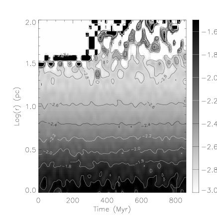
Figure 11: Slope of the mass distribution power-law as a function of time and radius in the cluster, for run m1. Since the low-mass stars are concentrated in the outer parts, they are preferentially stripped.

3.6 Mass segregation

It is well known that the mass distribution function for low-mass stars in an old globular cluster is very close to the IMF; this is specially true at the radius $r_{h}$, region which is more robust against mass segregation and tidal stripping (Vesperini, 1997), the two processes somewhat compensating at this radius to preserve the IMF. In the multi-mass King-Michie model that we adopted as initial conditions, the mass function varies with radius, as sketched in Fig. 12. It is also expected that the tidal stripping increases the mass segregation, in acting together with the relaxation of the central parts. Since the envelope is preferentially populated by low-mass stars, they are more stripped than the high-mass ones. This is shown in Fig. 11, where the value of the slope of the mass function is plotted (in gray-scale and in contours) as a function of time and radius in the cluster. Core relaxation is a way to replenish the low-mass stars content of the envelope. Recent HST results have discovered that some globular clusters have indeed mass functions depleted in low-mass stars (Sosin & King 1997, Piotto et al. 1997); the depleted clusters are very likely candidates for recent tidal shocking, from their presumed present galactic position and orbit (Dauphole et al. 1996).

The evolution through its dynamical life of the mass function of a globular cluster has been widely studied, in the goal of deriving the IMF slope at low mass of the galactic halo itself, which has important implications for the nature of dark matter. Gnedin & Ostriker (1997) showed that about 75% of the present globular cluster population will be destroyed in a Hubble time, and therefore that the majority of initial clusters is now destroyed and forms a large fraction of the stellar halo and bulge. Vesperini (1998), using an analytical scheme for the destruction processes, estimated the initial population of globular clusters to be about 300 clusters and the contribution of disrupted clusters to the halo would be about $5.5\leavevmode\nobreak\ 10^{7}M_{\odot}$, of the same order as the stellar mass in the halo (Binney & Merrifield, 1998). This means that the remaining clusters must have evolved considerably, and in particular their mass function. Capaccioli et al. (1993) have observed that the mass function slope is correlated with the position of the globular cluster in the galactic plane, and in particular with its height. The mass function is steeper at large distance. They show through analytical and N-body calculations that this could be due to disk shocking, that flattens the mass function. Johnston et al. (1999) have studied through N-body simulations the mass loss rates in mass-segregated systems. They confirm that the mass function is considerably flattened during tidal evolution; the slope x can fall from 1.35 to almost 0 for the more tide-vulnerable cases (small clusters in disk orbits).

Figure 12: Mass distribution function at different radii for model m2 (without rotation). The mass spectrum inside the radius containing 10% of the mass is compared with that outside the radius containing 90% of the mass. Dash lines correspond to the beginning of the simulation, and full lines at the end.

3.7 Tidal tails

Once the particles are unbound, they slowly drift along the globular cluster path when they were launched, and form a huge tidal tail. They can still form a recognizable features well outside the cluster envelope, and hundreds of pc away, as is observed on the sky (Grillmair et al. 1995, Leon et al. 1999). The tidal tails for 9 different models are displayed in Fig. 13, at the same spatial scale.

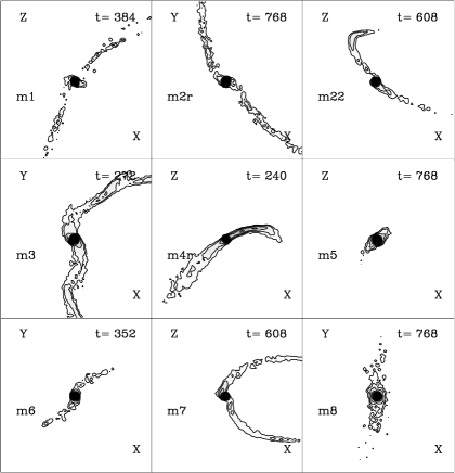
Figure 13: Contours of the projected density of particles (either onto xy, or xz planes) in logarithmic scale, with various clipping to show the tidal tails for the 9 different models indicated. Each square is 3.6 kpc in size. The epoch is indicated in Myr.

The unbound particles, and therefore the tails, are a tracer of the cluster orbit. The tails look asymmetrical, with a heavier tail on one side with respect to the other, but this is a projection effect, due to the particular shapes of the tails. There are sometimes special wiggles at the basis of the tails, in the cluster envelope, that are not due to the rotation of the clusters, since they are seen around non-rotating clusters as well (Fig. 13). These will be interpreted in Section 3.8.

Analysis of the faint tails is best performed with the wavelet decomposition, that can achieve multi-resolution, as in Fig. 14. The tidal tails can contain a few percents of the mass of the cluster. Fig. 13, 14 and especially Fig. 20 show the clumpy structure in the tidal tails. The denser unbound clumps are the tracers of the strongest phase of the gravitational shocks: the two symmetrical counterparts are visible on each side of the tails. Although these clumps are not bound, but transient caustics, the structure of the tail remains clumpy all over the simulations, even if it is not the same stars in the same clumps. We have followed in the simulations a group of particules that formed a clump at a given epoch: the group stays together for some time, until the packet of particules moves away from the cluster, then another clump is formed by a new tidal shock. It takes more than 800 Myr for a clump to disperse. A typical clump can contain 0.5% of the cluster stars. Some observed clusters (Leon et al. 1999) show evidence for such features in their tidal tails (e.g. NGC 5264, Pal 12). These overdensities in tidal tails are related to the ”streamers” or moving groups in the halo (Aguilar, 1997). These symmetrical features have been detected as well for open clusters oscillating in the galactic plane (Bergond et al. 1999).

How close tails trace the globular cluster orbit can be clearly seen on Fig. 15, showing a large-scale view of the globular cluster of the run m4, in a disk-like orbit. This cluster experienced strong disk shocks, due to the thin-disk model chosen, and was disrupted in 0.5 Gyr.

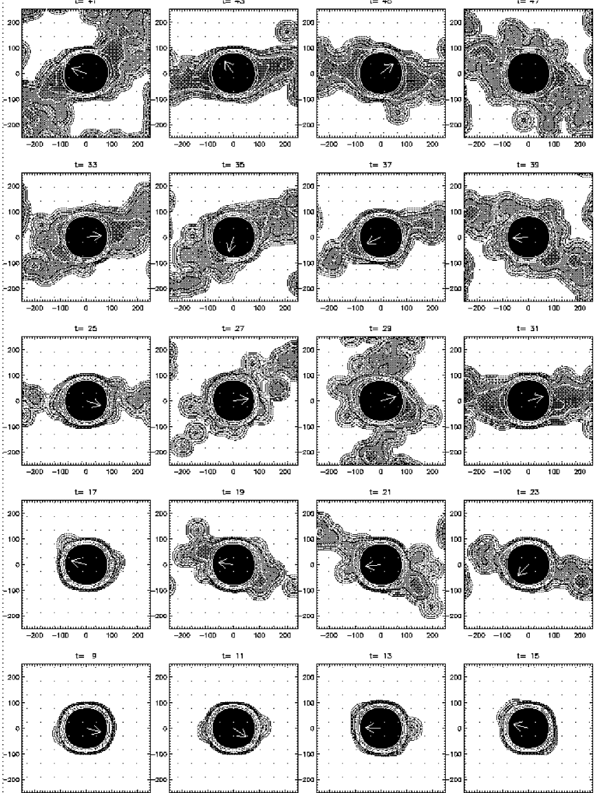
Figure 14: Tidal tails mapped at different epochs with the wavelet algorithm, for the model m2; the direction of the galactic center is indicated by the arrow. The maps are projected in the (X,Z) axes, OZ being perpendicular to the galactic plane.

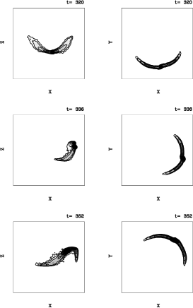
Figure 15: Contours of the projected density of particles in the run m4, in the logarithmic scale, showing the fate of the globular cluster in the thin-disk galaxy model. The squares shown are 8 kpc across, centered on the galactic center. The huge tidal tails trace perfectly the cluster orbit, even the loops in the x-z projection. Time is indicated in Myr.

Unbound particles, outside the tidal radius of the cluster, spread out in density like a power law, with a slope in average of –4. (Fig. 16). This kind of behaviour has been found for tidal extensions in numerical simulations of interacting galaxies (cf Aguilar & White 1986), and is that expected of an unbound cloud of particles in an 1/r potential, with a continuous spread in energy (with an almost constant probability, N(E), since then N(r)dr $\propto\rho r^{2}dr\propto$ N(E)dE $\propto r^{-2}$) starting from just zero relative energy, since at large distance, the globular cluster can be considered as a point mass, with 1/r potential. It does not depend on the source of the mass loss, and not significantly on the Galaxy potential either, since the latter gradients develop on larger scales.

The corresponding surface density around the cluster falls as $r^{-3}$ or steeper, which is far from the predictions of Johnston et al. (1999) for independent tidal debris, free to move and spread in the Galaxy potential: their expected slope of surface density is –1. Although these particles are in majority unbound to the cluster (have positive energy, as defined in Section 3.2), they cannot be considered as completely free, but still under the influence of the cluster potential; in particular, the closest ones can still be re-captured by the cluster. The discrepancy with the observations (Grillmair et al. 1995, Leon et al. 1999) where most of the slopes are around –1 is likely the consequence of noisy background-foreground subtraction.

Figure 16: Density profiles of two of the runs (m2 and m8), at t=768 Myr, both as a function of radius (left) or radius log (right). The dash line is the density at t=16 Myr for comparison. Note the clear change of slope at the tidal radius $r_{t}$. The slope in volumic density of the tail is around –4 (and in surface density, –3).

3.8 Flattening

At smaller scale, closer to the tidal radius, the just escaping particles are in general oriented perpendicular to the plane, just after a disk crossing. Monitoring the flattening of the cluster can be done through a Fourier analysis. Fig. 17 shows the resulting of even harmonics ($m=$ 2, 4, and 6) of the surface density projected in the plane, or perpendicular to the plane. When the cluster has no rotation, periodic compression of the cluster at its crossing of the plane, and subsequent relaxation, corresponding sometime in an extension of the cluster in the vertical direction is easily seen through the orientation of density maxima.

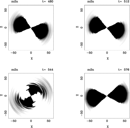
Figure 17: Fourier components (even harmonics $m=$2, 4 and 6) of the surface density projected into the x-z plane for the model m22 (no rotation). The scale is in pc, and time is in Myr.

In the case of a rotating cluster (m2r), the flattening in the xz plane is dominated by the rotation, although it varies slightly at the disk crossings. In the equatorial plane (xy), there is also an $m=2$ perturbation, which appears to tumble in the sense of rotation (Fig. 18).

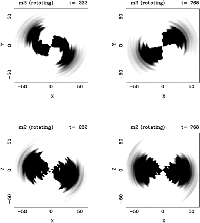
Figure 18: Fourier components (even harmonics $m=$2, 4 and 6) of the surface density projected into the x-z plane, and x-y plane for the model m2r (with rotation).

To better characterize the deformation of the globular cluster and the direction of the flattening, we have computed the (3x3) inertia momentum tensor

$$I_{xy}={{\Sigma_{n}m(n)xy/r^{2}}\over{\Sigma_{n}m(n)}}$$

with all combinations (x,y,z) taken into account. This computation is carried out on the globular cluster and its immediate envelope and avoids the tidal tails. The diagonalisation of this matrix gives the three eigen values plotted in Fig. 19 and the eigen vectors give the orientation of the major axis ($\theta$ and $\phi$ in spherical coordinates). In most of the models the eigen values are all almost equal to 1/3 (no large perturbations with respect to spherical shape). In the most perturbed cases, it is possible to see a clear prolate shape (the two almost equal axes are the smallest ones) with the major axis, located at an almost constant angle with the z-direction, and precessing around this z-axis (perpendicular to the plane) with retrograde sense (see Fig. 19). Some bouncing effects can also be noted, for example in model m4. The period of precession does not depend on the nature of the orbit, and has nothing to do with the time-scale between two crossings of the plane (it is in general much larger). On the contrary, the periods are similar for runs with the same initial state for the clusters. We interprete this period as an eigen value of the cluster itself: once a perturbation is excited, it develops with these proper frequencies (see e.g. Prugniel & Combes 1992).

Figure 19: The three eigen values of the inertia tensor, as a function of time (top), together with the ($\theta$, $\phi$) orientation of the major axis in spherical coordinates (middle and bottom, in radians) for the model m3 (left) and for the model m4 (right).

It is interesting to remark that this prolate shape taken by the globular clusters due to the tidal forces orients the mass loss just at the beginning of the tidal tails: unbound stars preferentially escape in the direction of the major axis, which gives the crooked shape of the global tail, that follows at large scale the cluster orbit (see Fig. 20).

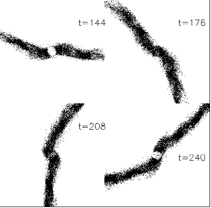
Figure 20: Plot of the particles just outside the tidal radius, at four epochs of the run m4 (in Myr). The particles inside the tidal radius of 85pc have not been plotted, for clarity. The particles are projected on the x-y galaxy plane.

4 Conclusions

We have carried out about a dozen N-body simulations of the tidal interactions between a globular cluster and the Galaxy, in order to characterize the perturbations experienced at disk crossing, to determine the geometry and density distribution of the tidal tails and quantify the mass loss as a function of cluster properties and Galaxy models. Our main conclusions can be summarised as follows:

• All runs show that the clusters are always surrounded by tidal tails and debris, even those that had only a very slight mass loss. These unbound particles distribute in volumic density like a power-law as a function of radius, with a slope around –4. This slope is much steeper than in the observations where the background-foreground contamination dominates at very large scale.

• These tails are preferentially composed of low mass stars, since they are coming from the external radii of the cluster; due to mass segregation built up by two-body relaxation, the external radii preferentially gather the low mass stars.

• The mass loss is enhanced for a cluster in direct rotation with respect to its orbit. No effect is seen for retrograde rotation.

• For sufficiently high and rapid mass loss, the cluster takes a prolate shape, whose major axis precess around the z-axis.

• When the tidal tail is very long (high mass loss) it follows the cluster orbit: the observation of the tail geometry is thus a way to deduce cluster orbits. Stars are not distributed homogeneously through the tails, but form clumps, and the densest of them, located symmetrically in the tails, are the tracers of the strongest gravitational shocks.

• Mass loss is highly enhanced with a “maximum disk” model for the Galaxy. On the contrary, the flattening of the dark halo has negligible effect on the clusters, for a given rotation curve.

Finally, these N-body experiments help to understand the recent observations of extended tidal tails around globular clusters (Grillmair et al. 1995, Leon et al. 1999): the systematic observations of the geometry of these tails should bring much information on the orbit, dynamic, and mass loss history of the clusters.

- (1) Aguilar L.: 1997, in “ ”Galaxy Interactions at low and high redshift” IAU Symposium 186, Kyoto, Japon, ed. D. Sanders, p. 8
- (2) Aguilar L., Hut P., Ostriker J.P.: 1988, ApJ 335, 720
- (3) Aguilar L., White S.D.M.: 1986, ApJ 307, 97
- (4) Allen A.J., Richstone D.O.: 1988, ApJ 325, 583
- (5) Bergond G., Leon S., Guibert J.: 1999, in prep
- (6) Binney J., Merrifield M.: 1998, “Galactic Astronomy” Princeton Series in Astrophysics, Princeton University Press.
- (7) Capaccioli M., Piotto G., Stiavelli M.: 1993, MNRAS 261, 819
- (8) Chernoff D., Kochanek C., Shapiro S.: 1986, ApJ, 309, 183
- (9) da Costa G.S., Freeman K.C.: 1976, ApJ 206, 128
- (10) Dauphole B., Geffert M., Colin J. et al.: 1996, A&A 313, 119
- (11) Davoust E., Prugniel P.: 1990, A&A 230, 67
- (12) Dejonghe H.: 1986, Phys. Rep. 133, 217
- (13) de Zeeuw T., Pfenniger D.: 1988, MNRAS 235, 949
- (14) Drukier G.A., Slavin S.D., Cohn H.N., et al.: 1998, AJ 115, 708
- (15) Fich M., Tremaine S.: 1991, ARAA 29, 409
- (16) Freeman K.C., Norris J.: 1981, ARAA 19, 319
- (17) Frenk C.S., Fall S.M.: 1982, MNRAS 199, 565
- (18) Gnedin O.Y., Ostriker J.P.: 1997, ApJ 474, 223
- (19) Gnedin O.Y., Ostriker J.P.: 1999, ApJ 513, 626
- (20) Gnedin O.Y., Hernquist L., Ostriker J.P.: 1999, ApJ 514, 109
- (21) Gnedin O.Y., Lee H.M., Ostriker J.P.: 1998, astro-ph/9806245
- (22) Grillmair C.J., Freeman K.C., Irwin M., Quinn P.J.: 1995, AJ 109, 2553
- (23) Haywood M., Robin A.C., Creze M.: 1997 A&A 320, 428
- (24) Hénon M.: 1961, Ann. d’Ap. 24, 369
- (25) Hernquist L., Ostriker J.P.: 1992, ApJ 386, 375
- (26) Hut P., Djorgovski S.: 1992, Nature 359, 806
- (27) Innanen K.A., Harris W.H., Webbink R.F.: 1983, AJ 88, 338
- (28) James R.A.: 1977, J. Comput. Phys. 25, 71
- (29) Johnston K.V., Sigurdsson S., Hernquist L.: 1999, MNRAS 302, 771
- (30) Keenan D.W.: 1981, A&A 95, 340
- (31) Keenan D.W., Innanen K.A.: 1975, AJ 80, 290
- (32) Kim S.S., Lee H.M., Goodman J.: 1998, ApJ 495, 786
- (33) King I.R.: 1962, AJ 67, 471
- (34) Kundić T., Ostriker J.P.: 1995, ApJ 438, 702
- (35) Lagoute C., Longaretti P-Y.: 1996, A&A 308, 441
- (36) Lee H.M., Goodman J.: 1995, ApJ 443, 109
- (37) Leon S., Meylan G., Combes F.: 1999, A&A preprint
- (38) Long K., Ostriker J.P., Aguilar L.: 1992, ApJ 388, 362
- (39) Longaretti P-Y., Lagoute C.: 1997a, A&A 308, 453
- (40) Longaretti P-Y., Lagoute C.: 1997b, A&A 319, 839
- (41) Makino J.: 1996, ApJ 471, 796
- (42) Merritt D., Meylan G., Mayor M.: 1997, AJ 114, 1074
- (43) Meylan, G., Mayor, M.: 1986, A&A 166, 122
- (44) Michie R.W.: 1963, MNRAS 125, 127
- (45) Nordquist H.K., Klinger R.J., Laguna P., Charlton J.C.: 1999, MNRAS 304, 288
- (46) Oh K.S., Lin D.N.C., Aarseth S.J.: 1992, ApJ 386, 506
- (47) Oh K.S., Lin D.N.C.: 1992, ApJ 386, 519
- (48) Oh K.S., Lin D.N.C., Aarseth S.J.: 1995, ApJ 442, 142
- (49) Ostriker J.P., Binney J., Saha P.: 1989, MNRAS, 241, 849
- (50) Piotto G., Cool A.M., King I.R.: 1997, AJ 113, 1345
- (51) Prugniel P., Combes F.: 1992, A&A 259, 25
- (52) Richer H.B., Fahlman G.G., Buonanno R. et al.: 1991, ApJ 381, 147
- (53) Sackett P.D., Sparke L.S.: 1990, ApJ 361, 408
- (54) Sackett P.D., Rix H-W., Jarvis B.J., Freeman K.: 1994, ApJ 436, 629
- (55) Sosin C., King I.R.: 1997, AJ 113, 1328
- (56) Spitzer L.J., Chevalier R.A.: 1973, ApJ, 183, 565
- (57) Spitzer L.J.: 1987, Dynamical Evolution of Globular Clusters, Princeton Series in Astrophysics
- (58) Takahashi K., Portegies Zwart S.F.: 1999, ApJ preprint (astro-ph/9903366)
- (59) Vesperini E.: 1997, in “The Combination of Theory, Observations, and Simulation for the Dynamics of Stars and Star Clusters in the Galaxy”, 23rd meeting of the IAU, Joint Discussion 15, 25 August 1997, Japan, p. 12
- (60) Vesperini E.: 1998, MNRAS, 299, 1019
- (61) Weinberg M.D.: 1994a, AJ 108, 1398
- (62) Weinberg M.D.: 1994b, AJ 108, 1403
- (63) Weinberg M.D.: 1994c, AJ 108, 1414
- (64) Wilson C.P.: 1975, AJ 80, 175