Extragalactic planetary nebulae as mass tracers: biases in the estimate of dynamical quantities

Abstract

Planetary nebulae (PNe) are very important kinematical tracers of the outer regions of early-type galaxies, where the integrated light techniques fail. Under ad hoc assumptions, they allow measurements of rotation velocity and velocity dispersion profile from descrete radial velocity fields. We present the results on the precision allowed by different set of radial velocity samples, discuss the hypotheses in the analysis of descrete velocity fields and their impact on the inferred kinematics of the stellar population.

Osservatorio Astronomico di Capodimonte, Naples, Italy

Osservatorio Astronomico di Capodimonte, Naples, Italy

Università “Federico II”, Naples, Italy

1. Introduction

With 4m telescopes and multi-object and/or multifiber spectrographs it has been possible to obtain information on the kinematics of the outer regions of ellipticals by measuring the radial velocities of individual stars during their phase of planetary nebulae. This is crucial because PNe are found at very large distances from galaxy centers where kinematical measurements based on standard integrated stellar light techniques are no longer possible. These radial velocity samples obtained from the PNe 5007 Å[OIII] emission in giant Es and S0s (D=15-17 Mpc) contain up to 50 PNe radial velocities (Arnaboldi et al. 1998), and larger samples are available only for nearer objects (i.e. NGC 5128, Sombrero, NGC 3115). Therefore there might be biases introduced by small number statistics that need to be investigated and understood.
Based on a statistical approach, we investigate the possibility of re-building the actual kinematics of spherical systems starting from descrete radial velocity fields. We build equilibrium systems for which dynamical and kinematical parameters are known (spherical model + known velocity field). By Montecarlo simulations we produce 100 “observational sets”, each for a given sample size, i.e. 50, 150 or 500 randomly chosen stars, and then analyse each sample to determine the rotation curves and velocity dispersion profiles. We account also for the measuring errors ($\sim$30% of the maximum rotational velocity). The aim of this work is to address the following questions: what is it the precision allowed by the different statistical samples in determining the kinematical quantities? Furthermore, may the hypotheses on the internal rotational structure introduce any biases?

2. Model procedure

We assume a constant M/L ratio and the Hernquist model (Hernquist 1990) for the dimensionless mass density distribution

$$\rho(r)=N\frac{1}{2\pi r(1+r)^{3}}$$ (1)

where $r$ is in units of a core radius $a$ and $N$ is a normalisation constant chosen as to have a total mass M_t=1 within a distance of 18$a$ from the center ($\sim 10R_{e}$). The cumulative mass distribution is

$$M_{l}(x)=4\pi\int_{0}^{x}x^{\prime 2}\rho(x^{\prime})dx^{\prime}$$ (2)

In spherical models with dark matter, we consider an additional mass contribution coming from an isothermal halo, and can write the dark matter density as (Dubinsky & Carlberg 1991):

$$\rho_{d}(r)=\frac{M_{d}}{2\pi}\frac{d}{r}\frac{1}{(r+d)^{3}}$$ (3)

where $M_{d}$, $d$ and $r$ have the same meaning as in eq. (1). In eq. (3), we take $d=10a$ and $M_{d}=7.7.M_{l}$. The cumulative mass distribution is defined as in eq. (2) with total mass:

$$M_{t}(r)=M_{l}(r)+M_{d}(r).$$ (4)

The model for the rotational velocity is

$$V_{rot}(x)=\frac{V_{0}x}{\sqrt{r_{0}^{2}+x^{2}}}$$

where $V_{0}$ is the maximum rotational velocity, $r_{0}$ is a scale factor and $x$ is the distance from the rotational axis (cylindrical rotation).
The PNe distribution is computed taking into account the selection effects of the bright continuum background from the stars in the central region of the galaxy. This selects a projected radius $R_{lim}$ onto the sky plane out of which the PNe sample is complete.

3. The descrete radial velocity field

From the mass density in space, $\rho(r)$, we extract via Montecarlo a star at position $(x_{p},y_{p},z_{p})\,=\,(r_{p},\theta_{p},\phi_{p})$. We check if $R_{p}^{2}=X_{p}^{2}+Y_{p}^{2}$, where ($X_{p},Y_{p}$) are the star projected coordinate onto the Sky Plane, is greater that the $R_{lim}$, the completeness limit radius. In the 3D space, we assign to the selected star its velocity vector under the hypothesis of “local isothermal approximation”, i.e. the observed distribution of radial velocity profiles in Es are Gaussian with maximum deviation of 10% (Bender et al. 1994). This is consistent with taking F(r,v) as product of three Gaussians. The $\sigma_{r},\sigma_{\theta},\sigma_{\phi}$ components are derived from the Jeans equation with the adopted $\rho(r)$ for the mass distribution, assuming isotropy for the velocity ellipsoid and the adopted rotation curve.
Once the 3D velocity vector is computed, the radial velocity is derived by projection of the velocity vector along the line-of-sight. This procedure is iterated for all the stars in a given sample and the 2-D descrete velocity field $V_{obs}(X,Y)$ is derived; a 500 PNe sample is shown in fig.1.

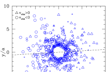
Figure 1.: A simulated radial velocity field: the dotted line indicates the direction of maximum gradient.

4. The analysis procedure

For each given V${}_{obs}(X,Y)$ sample, we perform a simple analysis of the velocity field as follows: we fit a rigid rotator (bilinear function) $v_{rad}=a+bX+cY$ and the results of this fit are compared with the results of a flat rotational curve fit (flat-fit) of the form $v_{rad}=v_{sys}+v_{0}\cos(\varphi-\varphi_{0})$ then we obtain the field of the residuals for each of the two interpolated fields $\Delta v=V_{obs}-v_{rad}$.
The aim of this procedure is to determine the characteristics of the velocity field: systemic velocity, direction of the maximum velocity gradient (Z1), velocity gradient and maximum rotational velocity. Along $Z1$, we select a slice of width $dZ1$ in order to trace the kinematics along this relevant axis; $dZ1$ must be small enough to trace the kinematics related to Z1 and large enough to allow a significant statistical sample. To describe the velocity dispersion profile, we analyse the residual fields from the two adopted fits, by computing averages along Z1 in bins, which contains at least 10 points.
As a check for the presence of biases, along the direction Z1 of maximum gradient, we obtain the rotation curve and the velocity dispersion profile simply as the average and radial velocity RMS in each of the given bins used in the analysis of the residuals, and we refer to this as the “No-fit” procedure.

5. Results and conclusions

As a first result we obtained that the direction of maximum gradient is independent of the rotational structure adopted for fit. For simulated samples with 500 PNe, the comparison between the simulated results with the expected model values show that the bilinear fit may introduce an over estimate of the velocity dispersion in the outer bins, depending on the intrinsic rotational structure of the galaxy. This bias is a function of the $v/\sigma$ ratio as shown in fig. 2. The no-fit procedure does not introduce biases in the determination of the velocity dispersion profile.

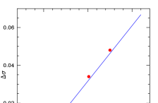
Figure 2.: The grey points are the values of the difference between the velocity dispersion determined in the last bin along Z1 and the expected value (weight average). The continuous line indicates the linear regression. The behaviour showed by the residuals indicates that higher rotation in the model causes the bilinear fit to introduce a larger bias in the velocity dispersion determination.

For samples with 50 PNe, in the outer bins we over-estimate the velocity dispersion by an amount which is dependent from the underlying mass distribution. If we take into account the weight effects in the binning, using the surface brightness distribution (i.e. surface density distribution via M/L ratio), we found a better consistency with the simulated data. The precisions obtained for the kinematical quantities depend on the selection performed along Z1. Our best mean estimate is 15% for 500 PNe and 22% for 50 PNe.
PNe can be used very efficiently as kinematical probes to trace the dynamics of the outer stellar halos in giant early-type galaxies provided that the analysis of the descrete radial velocity fields avoids any systematics depending on the assumption of the internal angular momentum distribution.

References

Arnaboldi, M., Capaccioli, M., Freeman, K.C. et al. 1998, ApJ, 507, 759

Bender, R. Saglia, R.P., Gerhard, O.E. 1994, MNRAS, 269, 785

Dubinsky, J., Carlberg, R.G. 1991, ApJ378, 496

Hernquist, L., 1990, ApJ, 356, 359