An Imaging and Spectroscopic Survey of
Galaxies within Prominent Nearby Voids I.
The Sample and Luminosity Distribution

Abstract

We study the optical properties of a large sample of galaxies in low-density regions of the nearby universe. We make a $5h^{-1}$ Mpc-smoothed map of the galaxy density throughout the Center for Astrophysics Redshift Survey (CfA2, Geller & Huchra (1989)) to identify galaxies within three prominent nearby “voids” with diameter $\gtrsim 30h^{-1}$ Mpc. We augment the CfA2 void galaxy sample with fainter galaxies found in the same regions from the deeper Century (Geller et al. (1997)) and 15R (Geller et al. (2000)) Redshift Surveys. We obtain $B$ and $R$ CCD images and high signal-to-noise longslit spectra for the resulting sample of 149 void galaxies, as well as for an additional 131 galaxies on the periphery of these voids.

Here we describe the photometry for the sample, including B isophotal magnitudes and $B\!-\!R$ colors. For the 149 galaxies which lie in regions below the mean survey density, the luminosity functions in $B$ and $R$ are well-fit by Schechter functions with respective parameters ($\alpha_{B}=-0.5\pm 0.3$, $B_{*}=-18.9\pm 0.2$) and ($\alpha_{R}=-0.9\pm 0.3$, $R_{*}=-20.4\pm 0.3$). The $B$ luminosity function (LF) is consistent with typical survey LFs (e.g. the Southern Sky Redshift Survey; Da Costa et al. (1998)), and the $R$ LF is consistent with the Century Survey. The $B$ and $R$ LFs of 131 galaxies in the “void periphery”, regions between the mean density and twice the mean, have similar Schechter parameters. The CfA2 LF is inconsistent with both samples at the $3.5\sigma$ level.

When we narrow our analysis to the 46 galaxies in regions below half the mean density, the LF is significantly steeper: $\alpha\sim-1.4\pm 0.5$. The typical survey LFs are inconsistent with this subsample at the $\sim\!2\sigma$ level. The $B\!-\!R$ color distribution of galaxies in the lowest-density regions is also shifted significantly ($\sim\!3\sigma$) blue-ward of the higher density samples. The most luminous red galaxies ($R\lesssim-21$) are absent from the lowest density regions at the $2.5\sigma$ level.

1 Introduction

Wide-angle redshift surveys during the last decade have provided a picture of galaxies distributed within large, coherent sheets, with clusters embedded in these structures, bounding vast ($10^{5-6}$ Mpc³) and well-defined “voids” where galaxies are largely absent. The relationship between local density in these structures and galaxy properties are of interest for constraining galaxy formation models. One of the most obvious indications of environmental dependence is the morphology-density relation (e.g., Dressler (1980); Postman & Geller (1984)), which quantifies the increasing fraction of ellipticals and lenticulars with increasing local density. In the lowest density regions, the voids, the observational evidence of trends in morphological mix, luminosity distribution, star formation rate, etc., is still rudimentary because of the intrinsic scarcity of void galaxies and the difficulties in defining an unbiased sample for study. Here we use a broadband imaging and spectroscopic survey of a large optically-selected sample to compare “void” galaxies with their counterparts in denser regions.

A better understanding of the properties of void galaxies is useful to constrain proposed theories of galaxy formation and evolution. For example, the peaks–bias paradigm of galaxy formation in a flat, cold dark matter universe (Dekel & Silk (1986); Hoffman, Silk, & Wyse (1992)) predicts that the voids should be populated with “failed galaxies” identified as diffuse dwarfs and that the $3\sigma$ massive galaxies in voids should have extended, unevolved, low surface-brightness (LSB) disks like Malin I (Bothun et al. (1987)). Unfortunately for this theory, dwarf galaxies are observed to trace the distribution of the more luminous galaxies (Bingelli (1989)), the environments of the observed Malin 1-type objects are not globally underdense (Bothun et al. (1993)), and Hi searches in voids have not turned up LSB giants (Szomoru et al. (1996); Weinberg et al. (1991); Henning & Kerr (1989)). Two recent efforts to measure redshifts for faint galaxies toward nearby voids, one comprising 185 optically-selected galaxies (Kuhn, Hopp, & Elsässer (1997)) and the other comprising 234 emission-line objects selected from objective prism plates (Popescu, Hopp, & Elsässer (1997)), both failed to discover faint galaxies filling the voids. However, the sky coverage in both cases was modest.

Balland, Silk, and Schaeffer (1998) recently proposed a variation on the peaks–bias model in which collision-induced galaxy formation drives the morphological biasing. This new model quantitatively recovers the cluster morphology-density relation, predicts essentially no difference in the morphological mix from the field to the voids, and predicts that non-cluster ellipticals must have all formed at high redshift ($z\gtrsim 2.5$). Similarly, Lacey et al. (1993) have proposed a model for the evolution of the galaxy luminosity function (LF) in which the rate of star formation is controlled by the frequency of tidal interactions. Their model predicts that luminous galaxies should not have formed in underdense regions for want of tidal interactions to trigger star formation.

There have been few previous measurements of the galaxy LF in low density regions, i.e., in the voids. Park et al. (1994) found two indications of luminosity bias in volume-limited samples from the Center for Astrophysics Redshift Survey (Geller & Huchra (1989), hereafter CfA2). For samples with $B_{\rm lim}=-19.1$ and $-18.5$, the power spectrum for the brighter half of the sample has $\sim\!40\%$ larger amplitude, independent of scale. Furthermore, the lower-density regions appear to be deficient in the brightest galaxies ($B\sim-20$) at the $\sim\!2\sigma$ level. El-Ad and Piran (1997) mapped out voids in the Southern Sky Redshift Survey (Da Costa et al. (1998), hereafter SSRS2), comparable in depth to CfA2. They identify 61% of the survey volume out to $80h^{-1}$ Mpc as “voids”; this volume contains 19% of the fainter $B>-19$ galaxies in the sample but only 5% of the brighter $B\leq-19$ galaxies. The significance of this result is difficult to interpret, because the void-detection algorithm depends only on the brighter galaxies.

Bromley et al. (1998) also investigated the environmental dependence of the LF in their recent spectral analysis of the Las Campanas Redshift Survey (Shectman et al. (1996), hereafter LCRS). Their density discriminant is a friends-of-friends algorithm (Huchra & Geller (1982)) to separate cluster and group galaxies from the rest. Their absorption-line objects have a much shallower LF in lower-density regions ($\alpha=0.19$ versus $-0.40$), and they observed a strong LF dependence on spectral type coupled with a substantial change in the spectroscopic-type mix with local density (akin to the morphology-density relation).

Most previous studies of the properties of individual void galaxies have focused on emission line-selected and $IRAS$-selected objects in the Boötes void at $z\sim 0.05$ (Kirshner et al. (1981, 1987)), and all studies have been limited to a few dozen objects. Broadband multicolor imaging of 27 Boötes void galaxies (Cruzen, Weistrop, & Hoopes (1997)) showed that they are brighter on average than emission-line galaxies at similar redshift. Moreover, a large fraction ($\approx 40$%) of this sample shows unusual or disturbed morphology. Weistrop et al. (1995) obtained H$\alpha$ images for a subset of 12 galaxies and reported star formation rates ranging from 3–55 $\cal M_{\odot}$ yr^-1, with the most active galaxies producing stars at almost three times the rate found in normal field disk systems. This finding confounds the naive expectation for void galaxies in the Lacey et al. (1993) model.

Szomoru, van Gorkom, & Gregg (1996) surveyed $\sim\!1\%$ of the Boötes void volume in Hi with the VLA around 12 $IRAS$-selected void galaxies. They detected these galaxies along with 29 companions. Szomoru et al. (1996) then argue that the Boötes void galaxies are mostly late-type gas-rich systems with optical and Hi properties and local environments similar to field galaxies of the same morphological type. They conclude that the void galaxies formed as normal field galaxies in local density enhancements within the void and that the surrounding global underdensity is irrelevant to the formation and evolution of these galaxies. These findings are in concert with the conclusions of Thorstensen et al. (1995), who examined an optically-selected sample of 27 galaxies within a nearby CfA2 void. The fraction of absorption-line galaxies in their sample is typical of regions away from cluster cores, and the local morphology-density relation appeared to hold even within the global underdensity.

Our goal is to try to resolve some of the apparent inconsistencies among previous studies by collecting high-quality optical data for a large sample of void galaxies with well-defined selection parameters. We thus obtained multi-color CCD photometry and high signal-to-noise spectroscopy for $\sim\!150$ optically-selected galaxies within prominent nearby voids. We work from the CfA2 Redshift Survey, which has the wide sky coverage and dense sampling necessary to delineate voids for $cz\lesssim 10000$ km s^-1. These conditions are not met for the Boötes void, making the definition of Boötes void galaxies in previous studies harder to interpret.

Using a straightforward density estimation technique, we identify three large ($\gtrsim 30h^{-1}$ Mpc) voids within CfA2. In addition to the void galaxies from CfA2, we include fainter galaxies found in the same regions by the deeper Century Survey (Geller et al. (1997); hereafter CS) and 15R Survey (Geller et al. (2000)). At the cost of mixing $B$-selected and $R$-selected samples, we thereby gain extra sensitivity at the faint end of the void luminosity distribution.

Our large sample, which covers essentially the entire volume of three distinct voids, should afford better constraints on the morphology, luminosity distribution, and star formation rate of void galaxies. Moreover, our sample drawn from $B$- and $R$-selected redshift surveys may be more broadly representative than the previous studies of emission-line, IRAS-selected, and Hi-selected void galaxies.

Here we introduce the sample, describe the broadband imaging survey, and derive the void galaxy luminosity distribution and the broad-band color distribution as a function of local density. Grogin & Geller (2000, hereafter Paper II ) will address the morphologies and spectroscopic properties of the galaxies in our sample. In §2 we describe the selection of the void galaxy sample. We discuss the multiple redshift surveys involved, describe the density estimation technique for identifying voids, and show maps of the galaxy density field. Section 3 describes the observations, reduction, and photometry. In §4 we derive a method for fitting luminosity functions in $B$ and $R$ to our heterogeneous galaxy sample. We apply the method to various density cuts through the sample and compare with typical redshift survey LFs. We discuss our results in §5 and conclude in §6.

2 Sample Selection

In §2.1 we briefly describe the three redshift surveys, CfA2, Century, and 15R, from which we select the void galaxies for this study. In §2.2 we review the estimator of the smoothed galaxy number density field within CfA2 (Grogin & Geller (1998)). In §2.3 we display maps of the density field around voids in this study.

2.1 Redshift Surveys

The Center for Astrophysics Redshift Survey of galaxies in the Zwicky Catalog (Zwicky et al. 1961– (1968)) now contains more than 14000 homogeneous redshifts and is 98% complete to $m_{\rm Zw}\leq 15.5$ (where Zwicky estimated his catalog was complete) over the regions ($8^{\rm h}\leq\alpha_{1950}\leq 17^{\rm h}$, $0\arcdeg\leq\delta_{1950}\leq 50\arcdeg$: CfA2 North) and ($20^{\rm h}\leq\alpha_{1950}\leq 4^{\rm h}$, $-2\fdg 5\leq\delta_{1950}\leq 50\arcdeg$: CfA2 South). These redshifts are all contained in the Updated Zwicky Catalog (Falco et al. (1999), hereafter UZC), which also includes arcsecond coordinates for all objects with $m_{\rm Zw}\leq 15.5$. We use the coordinates and redshifts from the UZC as the basis for the density field estimation of §2.2.

The Century Survey is a complete photometric and spectroscopic survey covering the region $8^{\rm h}30^{\rm m}\leq\alpha_{1950}\leq 16^{\rm h}20^{\rm m}$ and $29\arcdeg\leq\delta_{1950}\leq 30\arcdeg$ (0.03 steradians) to a limiting $m_{R}=16.13$. The CS catalog was constructed from POSS E plate scans (Kurtz et al. (1985)) and calibrated with drift-scan and pointed CCD photometry. The best-fit Schechter (1976) luminosity function to the 1762 CS galaxies has $M_{*}=-20.73\pm 0.18$ and $\alpha=-1.17\pm 0.19$. The CS $M_{*}$ is consistent with the red-selected Las Campanas Redshift Survey (Shectman et al. (1996), hereafter LCRS) of $>18000$ galaxies. The faint-end slope of the LCRS is significantly shallower than the CS: $\alpha_{\rm LCRS}=-0.70\pm 0.05$. This discrepancy may arise from the additional central surface-brightness cut used in LCRS, which may preferentially reject the faintest galaxies. Strong dependence of $\alpha_{\rm LCRS}$ on spectral type may also be the explanation, as suggested by Bromley et al. (1998). Similarly deep blue-selected surveys such as AUTOFIB (Ellis et al. (1996)) and the ESO Key Project (Zucca et al. (1997)) have faint-end slopes indistinguishable from the CS. We therefore take the CS as our fiducial $R$ galaxy LF in comparisons with the $R$ luminosity distribution of our void-selected samples.

The 15R Survey is an $R$-limited photometric and spectroscopic survey of two wider declination strips: ($8^{\rm h}30^{\rm m}\leq\alpha_{1950}\leq 16^{\rm h}30^{\rm m}$, $26\arcdeg 30\arcmin\leq\delta_{1950}\leq 32\arcdeg 30\arcmin$), which almost entirely overlaps the original CfA “Slice of the Universe” (de Lapparent, Geller, & Huchra (1986)); and a smaller region within CfA2 South ($20^{\rm h}\leq\alpha_{1950}\leq 4^{\rm h}$, $10\arcdeg 30\arcmin\leq\delta_{1950}\leq 13\arcdeg 30\arcmin$). The survey was originally intended to identify and measure redshifts of all galaxies down to a limiting $m_{R}=15.4$ in the 0.2 steradians covered by the survey. The photometric catalog was constructed from POSS E plate scans analogously to the CS, and plate magnitudes in 15R North were calibrated using galaxies common to both surveys. The Southern 15R survey magnitudes still require calibration: in §3.3.2 we use the photometry of our 15R South void galaxies to calibrate roughly the magnitude limit for each of the plates in 15R South.

Longslit CCD spectra of the 15R survey galaxies were obtained with the FAST spectrograph on the F. L. Whipple Observatory (FLWO) 1.5 m Tillinghast reflector over the period 1994–1997. The spectra were reduced as part of the Center for Astrophysics redshift survey pipeline and radial velocities were extracted via template cross-correlation (Kurtz & Mink (1998)). In the northern strip, the 15R redshift survey is complete to a limiting magnitude $m_{R}=15.42$. In the south, our calibrations indicate that most surveyed plates are complete to $m_{R}\approx 16$; none are shallower than $m_{R}\approx 15.4$.

2.2 Density Estimation Method

To identify regions of low galaxy density, we first transform the point distribution of the CfA2 survey into a continuously-defined number density field in redshift space. We smooth each CfA2 galaxy in redshift space with a unit-normalized Gaussian kernel $W$ of width $\sigma=5h^{-1}$ Mpc:

$$W\left({{\bf r}-{\bf r}_{\rm gal}}\right)=\left({2\pi\sigma^{2}}\right)^{-3/2}\exp\left({\left|{{\bf r}-{\bf r}_{\rm gal}}\right|^{2}/2\sigma^{2}}\right),$$ (1)

where ${\bf r}$ is the 3D redshift-space coordinate. We choose a $5h^{-1}$ Mpc smoothing length to coincide with the galaxy-galaxy correlation length (Peebles (1993); Marzke et al. (1995); Jing, Mo, & Boerner (1998)) and with the pairwise velocity dispersion in the survey (Marzke et al. (1995)).

We correct the redshift survey heliocentric velocities to the rest frame of the Local Group,

$$cz=cz_{\sun}+(300\,\hbox{\rm km s}^{-1})\sin l\cos b,$$ (2)

for a galaxy at Galactic longitude $l$ and latitude $b$. Otherwise, we make no attempt to remove peculiar velocity distortions (cluster “fingers”, etc.) from the redshift survey. We place each object at a comoving distance $r$ appropriate for a $q_{0}=0.5$ universe with pure Hubble flow:

$$r(z)=\left({{2c}\over{H_{0}}}\right)\left[{1-(1+z)^{-1/2}}\right].$$ (3)

For the low redshifts of interest here, $q_{0}$ has little effect on $r(z)$. Our smoothing kernel effectively washes out peculiar velocities $\lesssim 500$ km s^-1, close to the $540\pm 180$ km s^-1 pairwise velocity dispersion measured by Marzke et al. (1995) for the combined CfA2 and SSRS2. We underestimate spatial overdensities associated with clusters, which are broadened in the radial direction.

Because the CfA2 Redshift Survey is flux-limited, an increasing fraction of the galaxies at larger redshift fall below the magnitude limit and do not appear in the survey. In computing the density field, we compensate for the magnitude-limited sample by assigning each galaxy a weight $1/\psi$, where the selection function $\psi$ is

$$\psi(\alpha,\delta,z)={{\displaystyle\int_{-\infty}^{M_{\rm lim}(\alpha,\delta,z)}{\phi(M)\,dM}}\over{\displaystyle\int_{-\infty}^{M_{\rm cut}}{\phi(M)\,dM}}}.$$ (4)

Here $M_{\rm lim}$ is the effective absolute magnitude limit at the galaxy position and $\phi(M)$ is the differential luminosity function. For $M_{\rm lim}$ fainter than a fixed luminosity cutoff $M_{\rm cut}=-16.5$ (MHG (94)), we assign galaxies unit weight. Unless otherwise noted, all magnitudes in this section refer to Zwicky magnitudes. Numerical values for absolute magnitudes throughout this paper implicitly include the $h$-dependence in equation (3).

MHG (94) fit the CfA2 LF to a Schechter function $\phi_{\rm SF}$ (Schechter (1976)), convolved with a Gaussian error of $\sigma_{M}=0.35$ mag (Huchra (1976)) in the Zwicky magnitudes:

$$\phi_{\rm SF}(M) = \phi_{*}\,(0.4\ln 10)\,10^{0.4\,(M_{*}-M)\,(1+\alpha)}\exp\left[{-10^{0.4(M_{*}-M)}}\right];$$

$$\phi_{\rm CfA2}(M) = {1\over{\sqrt{2\pi}\sigma_{M}}}\int_{-\infty}^{\infty}{\phi_{\rm SF}(M^{\prime})\exp\left[{-(M^{\prime}-M)^{2}/2\sigma_{M}^{2})}\right]\,dM^{\prime}}.$$ (5)

We adopt the values $\phi_{*}=0.04\,({\rm Mpc}/h)^{-3}$, $M_{*}=-18.8$, and $\alpha=-1.0$ (MHG (94)). These values have not changed as a result of the revisions to the redshift catalog between 1994 and the release of the UZC (Marzke 1999). For computational convenience in determining $\psi$, we replace the convolution of equation (5) with $\phi_{\rm CfA2}(M)\approx\phi_{\rm SF}(M+0.1\,{\rm mag})$. This approximation recovers the true $\psi$ to better than 5% for $cz\lesssim 12000$ km s^-1.

For a galaxy at position ($\alpha,\delta$) and at luminosity distance $D_{L}(z)=(1+z)\,r(z)$ in a survey of limiting apparent magnitude $m_{\rm lim}$, we estimate the absolute limiting magnitude $M_{\rm lim}$ according to

$$M_{\rm lim}(\alpha,\delta,z)=m_{\rm lim}-5\log\left[{{(1+z)\,r(z)}\over{1h^{-1}\,\rm{Mpc}}}\right]-25-\Delta m_{\rm K}(z)-\Delta m_{\rm ext}(\alpha,\delta).$$ (6)

In equation (6), $\Delta m_{\rm K}$ is a $K$-correction, and $\Delta m_{\rm ext}$ is a correction for Galactic extinction. For the density estimation technique, $m_{\rm lim}$ represents the CfA2 flux limit in Zwicky magnitudes. Photoelectric photometry of Zwicky galaxies (Takamiya, Kron, & Kron (1995)) suggests that Volume I of the Zwicky catalog goes $\approx 0.4$ mag fainter than the other volumes at the CfA2 magnitude limit, $m_{\rm Zw}=15.5$. To correct for this Volume I scale error, we adopt $m_{\rm lim}=15.9$ for all CfA2 North galaxies with $\delta\leq 14\fdg 5$.

Lacking precise morphological types for the majority of CfA2, we apply a generic $K$-correction appropriate for the median type Sab (Pence (1976)): $\Delta m_{\rm K}(z)=3z$ for the Zwicky magnitudes. To obtain the correction $\Delta m_{\rm ext}(\alpha,\delta)$ for Galactic extinction along a particular line of sight, we first interpolate the Hi map of Stark et al. (1992). We then convert from Hi to reddening with the relation $\left<{N({\rm H}{\sc i})/E(\bv)}\right>=4.8\times 10^{21}$ cm^-2 mag^-1 (Zombeck (1990)). We adopt an extinction law $\Delta m_{\rm ext}\equiv A_{B}=4.0E(\bv)$ (Zombeck (1990)).

We also employ equation (6) for the luminosity function fitting of §4. In that case, $m_{\rm lim}$ represents the limiting magnitude of the appropriate redshift survey (CfA2, 15R, or Century Survey), corrected to the isophotal magnitude system used here (cf. §§3.3.1 and 3.3.2). We again adopt generic $K$-corrections of $\Delta m_{\rm K}(z)=3z$ for the CCD $B$ magnitudes and $\Delta m_{\rm K}(z)=0.8z$ for the CCD $R$ magnitudes (Frei & Gunn (1994)). Because we are only interested in the 15R and CS galaxies within the CfA2 redshift range ($z\lesssim 0.05$), the error in the $K$-correction will be small in any case. We use $\Delta m_{\rm ext}\equiv A_{B}=4.0E(\bv)$ to correct for extinction in the CCD $B$ magnitudes, and $\Delta m_{\rm ext}\equiv A_{R}=2.8E(\bv)$ to correct the CCD $R$ magnitudes (Zombeck (1990)).

We compute the smoothed galaxy number density $n$ at a given point ${\bf r}\equiv(\alpha,\delta,r(z))$ by summing the contributions from all $i$ galaxies in the CfA2 survey:

$$n({\bf r}) = \sum_{i}{{W({\bf r}-{\bf r}_{i})}\over\psi_{i}}$$ (7)

$$= \sum_{i}{{W({\bf r}-{\bf r}_{i})\displaystyle\int_{-\infty}^{M_{\rm cut}}{\phi(M)\,dM}}\over{\displaystyle\int_{-\infty}^{M_{\rm lim}({\bf r}_{i})}{\phi(M)\,dM}}}$$

$$= \bar{n}\sum_{i}{{W({\bf r}-{\bf r}_{i})\over{\displaystyle\int_{-\infty}^{M_{\rm lim}({\bf r}_{i})}{\phi(M)\,dM}}}}.$$

For the CfA2 Survey, MHG (94) derive a mean density $\bar{n}\equiv\int_{-\infty}^{M_{\rm cut}}{\phi(M)\,dM}=0.07\,({\rm Mpc}/h)^{-3}$ with $M_{\rm cut}=-16.5$. This analysis yields a continuous field of dimensionless galaxy density contrast, $n({\bf r})/\bar{n}$, which we use as the basis of our void galaxy selection.

2.3 The Sample

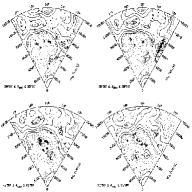
Figure 1: Cont’d.

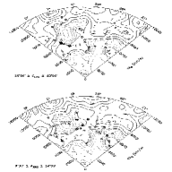
Figure 3: Cont’d.

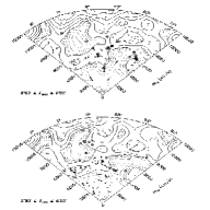
Figure 3: Cont’d.

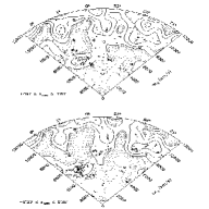
Figure 3: Cont’d.

We restrict our study to galaxies within three of the largest underdense regions in CfA2 ($\gtrsim 30h^{-1}$ Mpc diameter). This selection minimizes the contamination by interlopers with large peculiar velocities. Table 1 lists the approximate redshift-space boundaries of the three voids: “NV1” in CfA2 North, and in CfA2 South “SV1” (western) and “SV2” (eastern). In Figures 1 and 3 we display successive $3\arcdeg$ declination slices of CfA2 North and South, respectively, which contain NV1, SV1, and SV2. We superpose contours of the CfA2 galaxy density field $n$, with underdensities in linear decrements of $0.2\bar{n}$ (dotted contours) and overdensities in logarithmic intervals (solid contours) denoting $\bar{n}$, $2\bar{n}$, $4\bar{n}$, etc. The declination thickness of each slice exceeds the $5h^{-1}$ Mpc density smoothing length for $cz\gtrsim 10,000$ km/s; at lower redshifts there is density-field redundancy between adjacent slices. We indicate the locations of CfA2 galaxies with crosses and the subset chosen for this study with larger circles.

We attempted to include all survey galaxies within the $(n/\bar{n}=1)$ contour around each of the three voids. We define these galaxies as the “full void sample”, hereafter FVS. Because the FVS includes $\approx 150$ galaxies, we also examine the properties of two FVS subsamples: the lowest-density void subsample (hereafter LDVS) of 46 galaxies with $(n/\bar{n}<0.5)$, and the complementary higher-density void subsample (hereafter HDVS) with $(0.5n/\bar{n}<1)$.

Our sample also includes some of the galaxies around the periphery of the voids where $n/\bar{n}>1$. Typically the region surrounding the voids at $1<n/\bar{n}<2$ is narrow (cf. Fig. 1), intermediate between the voids and the higher-density walls and clusters. An exception is in the eastern half of our southern region of interest (cf. Fig. 3), where this contour is comparatively wide. Although our void periphery sample (hereafter VPS) is far from complete, we have selected these galaxies based only upon their proximity to the voids. We thus should not have introduced any luminosity selection bias between the FVS and the VPS. We use the VPS as a higher-density reference for the FVS and its subsamples.

In Figure 7 we show declination slices of the combined CS and 15R North (top) and of 15R South (bottom) where they intersect the three voids, along with superposed CfA2 isodensity contours. We plot the same span in right ascension as the CfA2 slices, denoting the survey boundaries with radial dotted lines. We indicate the 15R galaxy locations with crosses, the CS galaxies with triangular crosses, and the subset chosen for the current study with larger circles. It is striking to note the absence of 15R North galaxies within the NV1 region. Unfortunately we do not include the four 15R galaxies in NV1 at $\alpha_{1950}\gtrsim 16^{\rm h}$ because the measurement of POSS plate 329 redshifts was completed near the end of the 15R survey, after most of the observations for this study. We therefore set the magnitude limit for our study in this section of 15R North ($\alpha_{1950}>15^{\rm h}58^{\rm m}$) to the CfA2 limiting magnitude limit $m_{\rm Zw}=15.5$ rather than the magnitude limit $m_{R}=15.42$ for the rest of 15R North. The apparent magnitude limit of the CS allows detection of galaxies in NV1 down to absolute magnitudes of $R\approx-18$, some three magnitudes fainter than $L_{*}$.

3 Observations and Photometry

We acquired Johnson-Cousins $B$ and $R$ images of the 297 galaxies in our sample (cf. Tab. 3 below) over the course of several observing runs at the FLWO 1.2 m telescope: May/June 1995, October 1995, March 1996, June 1996, September 1996, April 1997, June 1997, and September/October 1997. Typical exposure times for each galaxy were 300 s in $R$ and $2\times 300$ s in $B$. The median seeing was $\approx 2\farcs 0$ and varied between $1\farcs 4$ and $3\farcs 3$. In May/June 1995 we used a thick, front-side illuminated, Ford $2048\times 2048$ CCD. We read out the data in $2\times 2$ binned mode, giving an $\approx 11\arcmin$ field with $0\farcs 64$/pixel. For all following observations we used a thinned, back-side illuminated, antireflection-coated Loral $2048\times 2048$ CCD. Again we had $2\times 2$ binned readout to obtain an $\approx 11\arcmin$ field at $0\farcs 63$/pixel.

3.1 Reduction Steps

We reduced our images using IRAF with the standard CCDRED tasks, subtracting the overscan and bias, interpolating across bad columns and pixels, and dividing by nightly combined dome or twilight sky flat fields to correct for pixel-to-pixel sensitivity variations. The dark counts on both chips were negligible; thus we did not subtract dark frames in the reduction. We passed the flatfielded images through the COSMICRAYS task to remove cosmic ray hits above $\sim\!60$ counts or a 7.8% flux ratio. We then fit a world coordinate system (WCS) to each frame by matching stars from the US Naval Observatory UJ1.0 Catalog (Monet, Canzian, & Henden (1994)) against stars in each field that we extracted with the SExtractor program (Bertin & Arnouts (1996)) and placed onto a global tangent projection. The typical rms deviation in the matched UJ1.0 objects was $0\farcs 3$. We stacked the two $B$ frames for each galaxy using offsets determined from the fitted WCS and re-fit a WCS to the combined image.

For images taken under photometric conditions, we calibrated the photometry with $B$ and $R$ images of several photometric standard fields (Landolt (1992)) taken at varying air-mass throughout the night. To obtain our photometric solution, we used the PHOTCAL task to fit to an instrumental zero point term, an air-mass term, and a $B\!-\!R$ color term to the instrumental (large aperture) magnitudes of the standard stars as obtained with the PHOT task. The scatter in a photometric solution fit is typically 0.015–0.020 mag. Because of poor weather during much of our observing time in 1996 and 1997, roughly half our our images required follow-up photometric calibration.

For images taken under nonphotometric conditions, we calibrated the photometry with follow-up ”snapshot” images of the same fields taken during photometric conditions with the Loral CCD on the FLWO 1.2 m from 1996–1998. We used the same procedure to reduce these snapshots, typically 120 s exposures, as for the longer exposures, including WCS fitting. We then ran SExtractor on both the uncalibrated and calibration frames, extracting stars common to both images by WCS position-matching. This procedure yielded $\gtrsim 30$ calibration stars per frame, enabling us to the recover the magnitude zero-points of the nonphotometric images to $\lesssim 0.02$ mag. This uncertainty is commensurate with the typical scatter in the photometric solutions.

We used a modified version of the GALPHOT surface photometry package (Freudling (1993)) to obtain galaxy isophotal magnitudes from our flatfielded images. We first estimated and subtracted the sky background around the target galaxies by interactive marking of sky boxes on the images. Because our galaxies only span $\lesssim 2\arcmin$ within $10\arcmin$ images, we typically marked $\sim\!10,000$ sky pixels around each galaxy for local sky subtraction. All the galaxies in our sample are comparatively bright ($m_{B}\gtrsim 17.5$), high surface-brightness objects for which the isophotal magnitude uncertainty due to sky subtraction is at worst on par with the 0.02–0.03 mag uncertainties from the photometric calibration.

Next we interactively masked foreground stars near the galaxies with the IMEDIT task. In the few rare cases when a star appeared too close to a galaxy center for simple masking, we used the DAOPHOT package to model the image point spread function (PSF) and to interactively fit and subtract a scaled PSF from the star’s position. We then masked any obvious residual in the PSF-subtracted stellar core with IMEDIT.

We determined the galaxy surface brightness profiles with the IRAF isophotal analysis package ISOPHOTE, part of the Space Telescope Science Data Analysis System. The package’s contour fitting task ELLIPSE takes an initial guess for an isophotal ellipse, then steps logarithmically in major axis. At each step it finds the optimal isophotal ellipse center, ellipticity, and positional angle. Masked pixels are ignored by ELLIPSE. Because the ELLIPSE algorithm averages pixels within an elliptical annulus, it is capable of fitting isophotes out to a surface brightness well below the sky noise. Far enough from the galaxy center, the fitting algorithm will ultimately fail to converge, and ELLIPSE enters a non-fitting mode which fixes larger ellipses to be similar to the largest convergent isophote. We generally ran ELLIPSE non-interactively, but in cases where a peculiar galaxy surface brightness profile sent the task into non-fitting mode prematurely, we stepped through the isophote fitting interactively.

Rather than fitting $R$ isophotal ellipses to the galaxy $R$ images, we determined the galaxies’ $R$ aperture magnitudes through overlaid $B$ image isophotes. We transferred the $B$ isophotal ellipses using the images’ fitted WCS, thereby compensating for variations in image scale and orientation. As a final step, we color-corrected the resulting $B$ and $R$ surface-brightness profiles at each isophote with the color term from the photometric solution. We do not correct for internal extinction. Our limiting $B$ isophote was governed by the early images taken with the thick Ford CCD, which had less sensitivity in $B$ than the Loral CCD. These images could not be fit by ELLIPSE beyond $\mu_{B}\sim 26$ mag arcsec^-2; we adopt this limit for the entire sample. The uncertainty in the $\mu_{B}=26$ mag arcsec^-2 isophote is $\lesssim 0.15$ mag arcsec^-2 on the thick chip images and $\lesssim 0.05$ mag arcsec^-2 on the thin chip. Although this procedure gave us the detailed surface brightness profiles of each galaxy, we defer that analysis and focus here solely on the isophotal magnitudes and colors.

3.2 Magnitudes and Colors

Table 3 lists the isophotal $B$ magnitudes ($b_{B26}$) and corresponding $R$ aperture magnitudes ($r_{B26}$) for the galaxies in our study. The uncertainty in these magnitudes is conservatively $\approx 0.05$ mag. We empirically verified this error from photometry of galaxies imaged in more than one observing run. We segregate the table by survey: CfA2 (Zwicky catalog) galaxies followed by 15R galaxies followed by Century Survey galaxies. We note that some of the galaxies are common to more than one of these overlapping surveys. For each galaxy we also provide arcsecond B1950 coordinates, the redshift corrected to the local standard of rest (cf. eq. [2]), and our estimate of the $5h^{\rm-1}$-smoothed galaxy density $(n/\bar{n})$ at the galaxy location. The typical error in this large-scale density estimator is $\lesssim 0.1$ for $cz\lesssim 10000$ km s^-1 (Grogin & Geller (1998)).

In Figure 8 we plot the absolute magnitudes (as determined with eq. [6]) $B_{B26}$ (top) and $R_{B26}$ (bottom) versus the $(\hbox{$B\!-\!R$})_{B26}$ colors for galaxies in the VPS (upper panel), the HDVS (middle panel), and the LDVS (lower panel). For notational convenience, we shall refer to the absolute magnitudes henceforth as $B$ and $R$. We also superpose onto Figure 8b the histograms of the various samples’ $B\!-\!R$ distribution (solid lines). Clearly there is a shift toward bluer galaxies in the LDVS, although the VPS and HDVS samples have similar color distributions. A Kolmogorov-Smirnov (K-S) test between the VPS and LDVS colors gives only a 0.3% probability of their being drawn from the same underlying distribution. The corresponding probability for the VPS and HDVS colors is 55%, but only 3.2% between the HDVS and LDVS colors.

One concern in interpreting the color distributions is that the distribution of absolute magnitudes may differ from sample to sample. Thus we must investigate color-magnitude correlation as a possible source of the LDVS color shift in Figure 8. To model the effect of a color-magnitude correlation, we select galaxies from the VPS according to the LDVS $R$ luminosity distribution and then compare the resulting color distribution of the galaxies selected from the VPS (lower panel, dotted line) with the LDVS colors (lower panel, solid line). The clear difference between the solid and dotted histograms (K-S probability of 0.08%) demonstrates that the blueward shift of the LDVS is not attributable to a difference in the absolute magnitude distribution for the sample galaxies.

One may also be concerned by a possible systematic color difference between the $B$-selected and $R$-selected galaxies in these samples, i.e. an $R$-limited sample should include redder objects near the magnitude limit than a $B$-limited sample. In our study, the $R$-selected galaxies are from deeper surveys (15R and CS) than the $B$-selected galaxies from CfA2, and thus disproportionately populate the faint end of our $R$ magnitude range. We note from Figure 8b that the faintest $R$ galaxies are also slightly bluer in the mean: $\left<{\hbox{$B\!-\!R$}}\right>=1.11\pm 0.25$ mag for $R>-20$ mag compared with $\left<{\hbox{$B\!-\!R$}}\right>=1.32\pm 0.25$ mag for $R<-20$ mag. Because the intrinsically less luminous galaxies tend to be $R$-selected and these galaxies are not particularly red, we do not see the anticipated red-ward shift of the $R$-selected galaxy colors. A K-S test of the $B\!-\!R$ colors for the $B$-selected and $R$-selected galaxies cannot distinguish between the two distributions ($P_{\rm KS}=72$%). We therefore employ the overall color distribution, regardless of selection filter, in our derivation of the $B$ and $R$ LFs.

For an external check on our color distributions, we compare with the $B\!-\!R$ CCD colors of 193 galaxies from the Nearby Field Galaxy Survey of Jansen et al. (1999). Their survey also used the FLWO 1.2 m, and with an observing setup identical to ours. Their distribution of field galaxy colors is indistinguishable from the HDVS ($P_{\rm KS}=71$%), and is similarly skewed redward of the LDVS at the $\approx\!2\sigma$ confidence level ($P_{\rm KS}=5.6$%).

3.3 Calibration of Redshift Survey Limiting Magnitudes

To analyze the luminosity dyistribution of the void galaxies, we need to convert the various redshift survey limiting magnitudes into the isophotal system used here. This task is simplest for CfA2 and the Century Survey, where the entire survey is characterized by a single magnitude limit. For the northern 15R Survey, calibrated against the CS, we assume that the whole strip is again described by a single magnitude limit. We use galaxies in this survey to calibrate the 15R South magnitudes on a plate-by-plate basis and obtain the limiting $r_{B26}$ magnitude on each of the plates. Section 3.3.1 describes our calibration of the void galaxy Zwicky magnitudes. We examine the Century Survey and 15R magnitude calibrations in §3.3.2.

3.3.1 Calibration of Void Galaxy CGCG Magnitudes

There have been suggestions that Zwicky deviated from a Pogson scale when assigning magnitudes to his faintest ($m_{\rm Zw}\gtrsim 15$) galaxies (Bothun & Schommer (1982); Giovanelli & Haynes (1984)). Such a scale error would have a significant impact on luminosity functions derived for the CfA2 survey (cf. MHG (94)). The largest previous investigation of the faint CGCG magnitudes with CCD photometry was by Bothun & Cornell (1990), who studied 107 cluster spirals of which 66 have $m_{\rm Zw}\geq 15.0$. They found that in the mean, $m_{\rm Zw}$ corresponds well to $b_{B26}$ with a scatter of 0.31 mag, comparable to the scatter at brighter $m_{\rm Zw}$ (Huchra (1976)). Although Bothun & Cornell observed that the Zwicky magnitudes were not closely isophotal, they found a linear relation between the magnitude systems with a slope $db_{B26}/dm_{\rm Zw}=1.05\pm 0.05$, consistent with zero scale error.

From Table 3 we have 230 isophotal $B$ magnitudes of Zwicky catalog galaxies down to the estimated catalog completeness limit of $m_{\rm Zw}\leq 15.5$. Of that number, 165 have $m_{\rm Zw}\geq 15.0$ and furnish an excellent dataset with which to gauge the accuracy of Zwicky’s magnitude estimates near the CfA2 survey limit. Our sample is complementary to that of Bothun & Cornell because we look at CGCG galaxies outside of clusters, comprising both early and late types. In Figure 9 we plot $b_{B26}$ versus $m_{\rm Zw}$ for the $m_{\rm Zw}\leq 15.5$ galaxies (crosses) along with an additional 8 Zwicky galaxies with $m_{\rm Zw}=15.6$–15.7 (open squares) from 15R and CS. The solid line in the figure is $b_{B26}=m_{\rm Zw}$; the dotted line is a linear least-squares fit to our data (with one outlier at $>3\sigma$ removed), which has slope $1.09\pm 0.06$ and an offset of $+0.10\pm 0.03$ mag from $b_{B26}=m_{\rm Zw}$ at $m_{\rm Zw}=15.5$.

Our slope is consistent with the Bothun & Cornell (1990) measurement, and represents the detection of a modest (0.09 mag mag^-1) scale error in the faint Zwicky magnitudes at a $1.7\sigma$ significance. The scatter in the linear fit is 0.32 mag, remarkably close to the scatter found by Bothun & Cornell. We do not include the $m_{\rm Zw}>15.5$ galaxies in the fit because these galaxies are not in CfA2. We are chiefly interested in converting the CfA survey limit ($m_{\rm Zw}=15.5$) to the $b_{B26}$ scale. Even with only 8 galaxies at $m_{\rm Zw}>15.5$, we can see from Figure 9 that Zwicky, just as he claimed, included substantially fainter objects in his last two magnitude bins.

With the redshifts for these Zwicky galaxies (Tab. 3), we can also investigate the Zwicky magnitude error ($b_{B26}-m_{\rm Zw}$) as a function of absolute Zwicky magnitude $M_{\rm Zw}$ (Figure 10). The Spearman rank correlation between the magnitude error and $M_{\rm Zw}$ is a negligible 0.02. A linear least-squares fit to the points in Figure 10 (with $2\sigma$-clipping) yields a Zwicky absolute magnitude scale error of $0.06\pm 0.04$ mag mag^-1 with a scatter of 0.28 mag. Thus we conclude that the Zwicky’s magnitude estimation was not biased by the intrinsic brightness of the galaxy over the range $-20.5\lesssim M_{\rm Zw}\lesssim-18$.

MHG (94) found a highly significant discrepancy in the maximum-likelihood LF parameters $\alpha$ and $M_{*}$ between CfA2 North and CfA2 South subsamples, with the CfA2 North $M_{*}$ some $0.26$ mag fainter. In addition to the possibility that the shape of the $cz\lesssim 10,000$ km s^-1 LF really does vary between the two Galactic caps, the authors suggest a number of potential systematic differences between the North and South Zwicky magnitudes that could reproduce the discrepancy (cf. Fig. 6 of MHG (94)): scale error offset, zero-point offset, varying faint-end incompleteness, and variation in the estimated Zwicky magnitude scatter. For example, they suggest that a differential scale error of 0.1 mag mag^-1 coupled with modest extra incompleteness of $\sim\!15\%$ by $m_{\rm Zw}=15.5$ would bring the CfA2 North and South LFs into agreement.

Our sample is sufficiently large to constrain most of the proposed Zwicky magnitude discrepancies between northern and southern Galactic caps. We repeat the linear fit between $b_{B26}$ and $m_{\rm Zw}$ on subsamples of 84 CfA2 North galaxies and 146 CfA2 South galaxies. We summarize the results in Table 5. Although the differential slope and offset in the linear fits to the North and South $m_{\rm Zw}$ have relatively large errors, they have roughly equal and opposite effects on the North/South LF discrepancy (MHG (94)). It is curious that the CfA2 North galaxies in our study have a noticeably smaller scatter than in CfA2 South (0.24 mag versus 0.35 mag). Huchra (1976) did not see this north/south difference in scatter with a somewhat smaller sample of photoelectric photometry. Bothun and Cornell (1990) did not address the issue. If the reduced dispersion is representative of the entire CfA2 North, this difference would drive the North and South $M_{*}$ estimates closer, but only by $\sim\!0.1$ mag.

3.3.2 Calibration of Century Survey and 15R Magnitudes

For the 13 Century Survey galaxies in our study, we find a linear fit between $r_{B26}$ and $m_{\rm CS}$ with slope $1.13\pm 0.07$ mag mag^-1 and offset of $+0.08\pm 0.07$ mag at the CS limiting magnitude $m_{\rm lim,CS}=16.13$. The scatter in the fit is 0.18 mag, near the $\sim\!0.25$ mag scatter estimated by Geller et al. (1997) between the CS plate magnitudes and CCD calibrations. Table 6 summarizes these results, along with the 15R calibrations below.

15R North is calibrated from the Century Survey, thus we simply use the linear fit to the CS magnitudes to find the 15R North $r_{B26,\rm lim}$. The offset at the 15R North magnitude limit $m_{\rm lim,N15R}=15.42$ is $-0.01\pm 0.05$ mag. The scatter in the 15R North magnitudes about the Century Survey fit is 0.25 mag, not appreciably worse than the CS scatter.

The situation for 15R South is less straightforward because the survey is uncalibrated except for the measurements here. Seven of the 12 POSS plates containing 15R void galaxies in this study have four or more members (cf. Tab. 6). In these cases we fit a linear model for $r_{B26}$ as a function of $r_{\rm 15R}$. We find that the scatter about these plate-specific calibrations is typically low, $\sim\!0.1$ mag, but the number of galaxies involved is far too small to comment on the accuracy of the plate scan magnitudes.

Five other 15R South plates contain only one or two galaxies from our sample, giving us minimal constraints on those plates’ limiting magnitudes. For these plates we adopt a linear relation with fiducial slope 0.75 mag mag^-1 and passing through the single calibration datum or the mean of the two data as appropriate. Where there are two calibrators per plate, we see that the “scatter” of those points about the fiducial linear model is similar to the $N\geq 4$ plates. Although the $r_{B26,\rm lim}$ estimates for these plates are highly uncertain, there are only eight galaxies in our sample of $\sim\!300$ which are affected.

Figure 11 summarizes the results of our 15R calibrations. On the left we plot $r_{B26}$ versus $r_{\rm 15R}$ for all the 15R galaxies in our sample, with the (dotted) line $r_{B26}=r_{\rm 15R}$ for comparison. We represent galaxies from different plates with unique symbols as indicated in the figure. On the right we plot $r_{B26}$ versus the “corrected” 15R magnitudes $r_{\rm 15R^{\prime}}$ using the plate-specific linear models for 15R South galaxies and the CS linear model for the 15R North galaxies (from plates 324 and 325). The linear corrections are sufficient to bring the discrepant $r_{\rm 15R}$ into good agreement with $r_{B26}=r_{\rm 15R^{\prime}}$ (dotted line, right panel).

4 Luminosity Function Fitting

Here we use our two-color photometry to analyze the void galaxy luminosity function in both $B$ and $R$. Because we have drawn the sample from both $B$-selected and $R$-selected redshift surveys, however, the procedure for fitting a luminosity function is more involved than for a sample selected from a single magnitude-limited survey. We describe the technique in §4.1 and the results in §4.2.

4.1 Technique

We follow the method of Sandage, Tammann, and Yahil (1979, hereafter STY), who solve for an optimal parametric luminosity function $\phi$ by varying the parameters to maximize the likelihood of the observed luminosity distribution. With a sample of N galaxies located at $r_{i}$, the likelihood ${\cal L}$ is given by the product of the probability $p$ that the observed absolute magnitude $M_{i}$ of each is drawn from $\phi$:

$${\cal L}=\prod_{i=1}^{N}{p(M_{i},r_{i}|\phi)}=\prod_{i=1}^{N}{{\phi(M_{i})}\over{\int_{-\infty}^{M_{\rm lim}(r_{i})}{\phi(M)\,dM}}},$$ (8)

where $M_{\rm lim}$ is given by equation (6). The STY technique is particularly well-suited to our void sample because it is independent of the survey geometry, easily accommodates variations in survey magnitude limit, and is minimally biased by nonuniform density fields (Efstathiou, Ellis, & Peterson 1988, hereafter EEP ).

The STY likelihood of equation (8) assumes that the survey limiting magnitude at each galaxy location, $M_{\rm lim}(r_{i})$, is always in the same passband as the LF we are estimating. Our sample does not satisfy this assumption: our heterogeneous collection of void galaxies is drawn from surveys that are $B$-limited (CfA2) as well as $R$-limited (15R and CS). Rather than attempting to fit a bivariate LF in $B$ and $R$ to our modest sample, we use the color distribution of the sample to transform a limiting absolute magnitude in filter Y into an approximate distribution of limiting magnitudes in filter X as necessary. We then perform an appropriate summation in the denominator of equation (8) over this distribution of limiting magnitudes:

$$\sum_{j}^{n_{j}}{f\left[{(M_{X}\!-\!M_{Y})_{j}}\right]\times\int_{-\infty}^{M_{Y,{\rm lim}}(r_{i})+(M_{X}\!-\!M_{Y})_{j}}{\phi(M_{X})\,dM_{X}}},$$ (9)

where $f\left[{(M_{X}\!-\!M_{Y})_{j}}\right]$ is the fraction of sample galaxies with color $(M_{X}\!-\!M_{Y})_{j}$.

In practice, we set $f[(\hbox{$B\!-\!R$})_{j}]$ equal to the sample’s ($B\!-\!R$) histogram in 0.1 mag intervals (comparable to our color uncertainty for 5% photometry). As a purely notational convenience for the following derivations, we introduce the terms $B_{\rm lim}^{\rm eff}$ and $R_{\rm lim}^{\rm eff}$ as shorthand for the summation in (eq. [9]):

$$\int_{-\infty}^{B_{\rm lim}^{\rm eff}(r_{i})}{\phi_{B}(B)\,dB} \equiv \sum_{j}^{n_{j}}{f\left[{(B\!-\!R)_{j}}\right]\times\int_{-\infty}^{R_{\rm lim}(r_{i})+(B\!-\!R)_{j}}{\phi_{B}(B)\,dB}},$$

$$\int_{-\infty}^{R_{\rm lim}^{\rm eff}(r_{i})}{\phi_{R}(R)\,dR} \equiv \sum_{j}^{n_{j}}{f\left[{(B\!-\!R)_{j}}\right]\times\int_{-\infty}^{B_{\rm lim}(r_{i})-(B\!-\!R)_{j}}{\phi_{R}(R)\,dR}}.$$

This treatment assumes that within a given sample, there is negligible color-magnitude correlation in the data over the range of limiting absolute magnitude. One may worry that this assumption is violated by the data, as we have already seen in §3.2 that the color distribution is correlated with density environment. In fact there is little color-magnitude correlation in $B$ for any of the samples (Tab. 4). Although Table 4 shows that $R$ is more strongly correlated with $B\!-\!R$, the correlation largely vanishes for $R\gtrsim-20$, a range which includes all $R$-selected limiting magnitudes. Despite the color variation with density, we may safely assume that the colors and magnitudes remain uncorrelated, at least near the absolute magnitude limits, for any particular density subsample.

Inserting the cross-color magnitude limit correction (eq. [9]) into the likelihood equation (eq. [8]) and taking the logarithm, we arrive at the expression for the log-likelihood of the $B$ luminosity function $\phi_{B}$:

$$\ln({\cal L}_{B}) = \sum_{i}^{N}{\ln[\phi_{B}(B_{i})]}-\left\{{\sum_{i}^{N_{B}}{\ln\int_{-\infty}^{B_{\rm lim}(r_{i})}{\phi_{B}(B)\,dB}}}\right\}_{B-\rm selected}$$

$${}-\left\{{\sum_{i}^{N_{R}}{\ln\int_{-\infty}^{B_{\rm lim}^{\rm eff}(r_{i})}{\phi_{B}(B)\,dB}}}\right\}_{R-\rm selected},$$

where the numbers of $B$-selected and $R$-selected galaxies in the sample are respectively $N_{B}$ and $N_{R}$ ($=N-N_{B}$). Similarly, the log-likelihood of the $R$ luminosity function $\phi_{R}$ is given by:

$$\ln({\cal L}_{R}) = \sum_{i}^{N}{\ln[\phi_{R}(R_{i})]}-\left\{{\sum_{i}^{N_{R}}{\ln\int_{-\infty}^{R_{\rm lim}(r_{i})}{\phi_{R}(R)\,dR}}}\right\}_{R-\rm selected}$$

$${}-\left\{{\sum_{i}^{N_{B}}{\ln\int_{-\infty}^{R_{\rm lim}^{\rm eff}(r_{i})}{\phi_{R}(R)\,dR}}}\right\}_{B-\rm selected}.$$

The quantity $-2\ln({\cal L})$ for a parametric luminosity function of $n_{p}$ fitted parameters is distributed about its minimum as a $\chi^{2}$ with $(N-n_{p})$ degrees of freedom.

Although our photometry is accurate to $\approx 0.05$ mag, the magnitude limits appearing in equations (4.1) and (4.1) are derived from redshift survey magnitudes that have a much larger scatter. We correct for the resulting Malmquist bias by convolving the integrals in equations (4.1) and (4.1) with Gaussians in the limiting magnitudes of respective width $\sigma_{B}=0.35$ mag (appropriate for CfA2) and $\sigma_{R}=0.25$ mag (appropriate for 15R and CS).

We test our STY implementation with Monte Carlo realizations of the sample magnitudes. We preserve the sample’s heterogeneous selection criteria and draw colors from the sample’s $B\!-\!R$ distribution. We test both $B$ and $R$ input luminosity functions, using Schechter functions with parameters ($\alpha_{B}=-1.0$, $B_{*}=-18.8$) and ($\alpha_{R}=-1.17$, $R_{*}=-20.73$). In 1000 simulations of the FVS, we recover the input LF in both passbands to 0.03 in $\alpha$ and 0.02 mag in $M_{*}$ in the mean. The Monte Carlo parameter dispersion is consistent with the parameter confidence intervals predicted for the actual data (§4.2).

Although the STY technique can find the optimal parametric LF and its parameter uncertainties, it does not provide information about the goodness of fit. The goodness of fit is typically estimated by comparison of a nonparametric LF maximum likelihood with the parametric LF maximum likelihood (Eadie et al. (1971)). The most commonly used nonparametric LF is from the stepwise maximum-likelihood (SWML) method of EEP and consists of a series of steps $\phi_{k}$ at regular luminosity intervals $M_{k}$ separated by $\Delta M$.

The stepwise maximum likelihood found by independently varying the step heights $\phi_{k}$ is then compared, not to the STY maximum likelihood, but to the stepwise likelihood of the expected steps from $\phi_{\rm STY}$ (cf. eq. [2.15] of EEP ):

$$\phi_{k,\rm STY}\approx{{\int^{M_{k}+\Delta M/2}_{M_{k}-\Delta M/2}\phi_{\rm STY}^{2}10^{-0.6M}\,dM}\Bigg{/}{\int^{M_{k}+\Delta M/2}_{M_{k}-\Delta M/2}\phi_{\rm STY}10^{-0.6M}\,dM}},$$ (12)

where the approximation assumes that the survey volume in which galaxies of luminosity $L$ are seen above the magnitude limit scales as $L^{3/2}\propto 10^{-0.6M}$. This assumption is reasonable for the typical sample of galaxies from a single redshift survey to a given flux limit in a single passband within a simple spatial geometry. It is not accurate for our samples, which are restricted to disjoint irregular volumes at varying distances and drawn from multiple redshift surveys with varying sky coverage and magnitude limits in two filters.

Because of the difficulty in obtaining $\phi_{k,\rm STY}$ for our sample, we do not use SWML to evaluate the STY goodness of fit. Instead we directly compare the observed luminosity cumulative distribution function (CDF) of the data with the luminosity CDF $C(M|r_{i},\phi)$ predicted for the sample from the parametric LF. For the case of a sample selected in a single filter, the predicted luminosity CDF has the form

$$C(M|r_{i},\phi)={1\over N}\sum_{i}^{N}{\min\left({{{\int_{-\infty}^{M}{\phi(M^{\prime})\,dM^{\prime}}}\over{{\int_{-\infty}^{M_{\rm lim}(r_{i})}{\phi(M^{\prime})\,dM^{\prime}}}}},1}\right)}$$ (13)

By preserving the observed redshift distribution, this model-predicted luminosity CDF is independent of variations in the galaxy density. We introduce a cross-color correction to the magnitude limit (eq. [9]) in the denominator of (eq. [13]), analogous to our treatment of the likelihood equation (eq. [8]). We may then express the model-predicted luminosity CDF for a $B$ luminosity function as

$$C(B|r_{i},\phi_{B}) = \left\{{{1\over N_{B}}\sum_{i}^{N_{B}}{\min\left({{{\int_{-\infty}^{B}{\phi_{B}(B^{\prime})\,dB^{\prime}}}\over{\int_{-\infty}^{B_{\rm lim}(r_{i})}{\phi_{B}(B^{\prime})\,dB^{\prime}}}},1}\right)}}\right\}_{B-\rm selected}$$

$${}+\left\{{{1\over N_{R}}\sum_{i}^{N_{R}}{\min\left({{{\int_{-\infty}^{B}{\phi_{B}(B^{\prime})\,dB^{\prime}}}\over{\int_{-\infty}^{B_{\rm lim}^{\rm eff}(r_{i})}{\phi_{B}(B^{\prime})\,dB^{\prime}}}},1}\right)}}\right\}_{R-\rm selected},$$

where the $\min()$ operation on the ratio of integrals is to be performed within the summation implied by $B_{\rm lim}^{\rm eff}$. Swapping all instances of $B$ and $R$ in equation (4.1) yields the corresponding model-predicted luminosity CDF in $R$. As in our treatment of the STY technique, we account for the Malmquist bias of the redshift surveys by convolving the denominator integrals of $C()$ above with Gaussians in the limiting magnitude.

We compare an observed luminosity CDF with the model-predicted CDF $C(M|r_{i},\phi)$ using the Kolmogorov-Smirnov (K-S) test. From the resultant K-S $D$-statistic, we may obtain the probability $P_{\rm KS}(\phi)$ of the null hypothesis that the sample was drawn from $\phi$. Because our computation of $C()$ incorporates the observed color distribution via $M_{\rm lim}^{\rm eff}$, we cannot use the standard approximation for $P_{\rm KS}$ in terms of $D$ (cf. Press et al. (1992)). This limitation pertains even when comparing the observed luminosity CDF against the predictions from survey LFs (e.g., $\phi_{\rm SSRS2}$) with parameters not fit to our data. We explicitly compute the probability of the null hypothesis by generating the distribution of the K-S $D$-statistic between $C()$ and Monte Carlo realizations of the sample’s luminosity CDF. Our realizations satisfy the same absolute magnitude limits as the sample, with magnitudes drawn from the model LF and colors drawn from the sample’s color distribution.

4.2 Results

We carry out the LF analysis of §4.1 identically for the FVS ($n/\bar{n}<1$), the VPS ($1<n/\bar{n}<2$), the LDVS ($n/\bar{n}<0.5$), and the HDVS ($0.5<n/\bar{n}<1$). For each sample, we show separate figures for the $B$ and $R$ LF determination. The upper plot of each LF figure (Figs. 12a–19a) shows the joint-probability intervals (solid contours) of the Schechter function parameters $\alpha$ and $M_{*}$. We also display the likelihood intervals (dashed contours) which project onto the individual $n$-$\sigma$ bounds of $\alpha$ and $M_{*}$. For comparison with the maximum-likelihood parameters (plus symbol), we indicate the Schechter function parameters of various survey LFs. For $B$ we mark the CfA2 LF ($\alpha_{B}=-1.0$, $B_{*}=-18.8$; MHG (94)) with a square, the SSRS2 LF ($\alpha_{B}=-1.12$, $B_{*}=-19.43$; Marzke et al. (1998)) with a diamond, and the Stromlo-APM Redshift Survey LF ($\alpha_{B_{J}}=-0.97$, $B_{J,*}=-19.50$; Loveday et al. (1992)) with a cross. For $R$ we mark the Century Survey LF ($\alpha_{R}=-1.17$, $R_{*}=-20.73$; Geller et al. (1997)) with a triangle and the LCRS LF ($\alpha_{R}=-0.70$, $R_{*}=-20.64$; Lin et al. (1996)) with an asterisk.

The lower plot of each LF figure (Figs. 12b–19b) indicates the goodness of fit for various Schechter functions to the given sample’s luminosity CDF (jagged solid line). We overplot the model-predicted $C(M|r_{i},\phi)$ for our best-fit Schechter function (dotted curve) as well as the Schechter functions for various survey LFs. For $B$ we show the predictions for CfA2 (long-dashed curve) and SSRS2 (short-dashed curve). For $R$ we show the prediction for the Century Survey (dashed curve). In all cases we give the K-S probability (from Monte Carlo simulation) of the null hypothesis between the Schechter LF and the data. We summarize the results in Table 7.

Figures 12a and 13a show our results for the STY Schechter function analysis of the 149 galaxies comprising the FVS. The SSRS2 LF is brighter and steeper than the best-fit $B$ LF, but in the direction poorly constrained by the data ($\sim\!1.5\sigma$ exclusion). The CfA2 LF deviates less from the maximum-likelihood values, but in a better-constrained direction ($>3.5\sigma$ exclusion). For the $R$ LF, we find best-fit parameters close to the Century Survey LF, which lies within the 68% likelihood contour. Figures 12b and 13b show the goodness of fit of various Schechter functions to the FVS. We find a high K-S probability of the data being drawn from the either the best-fit $B$ Schechter function or the SSRS2 LF. The CfA2 Schechter function, however, significantly underestimates the fraction of bright galaxies actually observed and results in a $P_{\rm KS}(\phi_{\rm CfA2})=0.07\%$. The best-fit $R$ Schechter function predicts a luminosity CDF which is indistinguishable from the FVS $R$ magnitudes, as does the Century Survey LF. We find little evidence for an FVS luminosity distribution significantly fainter than typical survey LFs.

Figures 14a and 15a show the STY Schechter function analysis of the 131 galaxies comprising the VPS. The maximum-likelihood Schechter function parameters are highly consistent with the FVS (cf. Tab. 7) and similarly close to SSRS2 and CS. Figures 14b and 15b show the goodness of fit of various Schechter functions to our VPS. The K-S probabilities are close to those for the FVS: the VPS luminosity distribution is indistinguishable from the predictions of the optimal Schechter functions in each filter or from the survey LFs from SSRS2 and CS ($P_{\rm KS}\approx 60\%$). These results, which suggest that the VPS is in fact representative of the overall galaxy LF, appear to argue against significant LF variation between a general redshift survey and void galaxies. Again the CfA2 Schechter function is a very poor fit to the data. We discuss this issue in §5.

It is only when we look to the galaxies in the very lowest density regions that we see a deviation from typical survey LFs (SSRS2 and Century). Figures 16a and 17a show the STY analysis of the 46 galaxies comprising the LDVS. Although the parameter uncertainties are much larger in this smaller sample, we find a significantly steeper $B$ LF of $\alpha_{B}=-1.4\pm 0.6$. This subsample only excludes the SSRS2 LF at $\lesssim 2\sigma$, while the CfA2 LF is well within the $1\sigma$ likelihood contour. The maximum-likelihood $R$ LF has a similarly steep $\alpha_{R}=-1.4\pm 0.5$ and excludes the Century Survey LF at $\approx 2\sigma$.

Figures 16b and 17b show the goodness of fit of various Schechter functions to the LDVS. The K-S probability of the data being consistent with the best-fit $B$ Schechter function is reasonable ($<1\sigma$ discrepancy) although smaller than for the other samples. The probability of the CfA2 LF being consistent with the LDVS is comparably high, while SSRS2 LF is mildly discrepant ($P_{\rm KS}=16\%$). We see from Figure 16b that the SSRS2 LF overpredicts the observed CDF at essentially all magnitudes. All three Schechter LFs predict a steeper luminosity CDF around $B_{*}$ than we observe. The maximum-likelihood Schechter function in $R$ predicts a luminosity CDF consistent with the data ($P_{\rm KS}=66\%$), while the Century Survey LF overpredicts the fraction of bright galaxies. In this respect, the CS LF is more discrepant with the $R$ magnitudes ($P_{\rm KS}=3.5\%$) than SSRS2 in $B$.

In light of the steeper LDVS, it is not surprising that we see a shallower LF for the 103 galaxies comprising the complementary HDVS (Figs. 18a and 19a). As we found for the FVS, the HDVS discrepancy with SSRS2 and CS is in the poorly-constrained direction, while the CfA2 LF is strongly excluded ($>4\sigma$). Although the observed luminosity CDF is fit well by the $B$ and $R$ maximum-likelihood Schechter functions (Figs. 18b and 19b), the survey LFs underpredict the observed number of $\sim\!M_{*}$ galaxies at the $\sim\!2\sigma$ level.

An interesting feature of Figure 17b is the sharp cutoff of the LDVS CDF for the brightest red galaxies ($R<-21$). The survey LF predicts that $\approx 10\%$ of the sample should be brighter than the brightest observed $R$, a $>2.5\sigma$ discrepancy. We conclude from Figure 20 that there is evidence for a steepening in the faint-end slope of the void galaxy LF at the lowest densities and a relative deficit of red objects (cf. Fig. 8), particularly at the bright end.

5 Discussion

The luminosity distribution of 149 galaxies within underdense ($n<\bar{n}$) regions of CfA2 is very similar to the predictions of typical survey LFs from SSRS2 ($\alpha_{B}=-1.12$; $B_{*}=-19.43$) and the Century Survey ($\alpha_{R}=-1.17$; $R_{*}=-20.73$). The 131 galaxies in our study surrounding the voids at $\bar{n}<n<2\bar{n}$ also show a luminosity distribution consistent with these survey LFs. These two results (cf. Tab. 7), as well as the similarity in colors between the HDVS and the VPS (cf. Fig. 8), suggest that the influences of environment upon galaxy formation and evolution that shape a survey LF also pertain in regions of at least moderate global underdensity.

Oddly, the CfA2 LF as fit by MHG (94) is a poor match to the $B$ magnitudes of our higher-density samples, which are largely drawn from CfA2 but agree instead with the SSRS2 LF. The discrepancy of ($\Delta B_{*}\approx 0.6$ mag) between the LFs of these disjoint wide-angle surveys to similar depth ($m_{B(0)}\approx 15.5$) has recently received attention from Marzke et al. (1998). In fitting type-dependent LFs to SSRS2, they observe a deficit of bright CfA2 galaxies across all morphological types and suspect some systematic error in the Zwicky magnitudes. Our CCD photometry of 230 CGCG galaxies places the best current limits on such errors.

Our CfA2 North magnitudes do have a lower scatter (0.24 mag) than the 0.35 mag assumed by MHG (94) when fitting the CfA2 LF, although this effect would only brighten the North LF by $\sim\!0.1$ mag. We see a modest faint-end CGCG scale error of $0.09\pm 0.06$ mag mag^-1 and zero-point offset of $\lesssim 0.10\pm 0.03$ with an overall scatter of 0.32 mag. Our scale error and zero-point offset have roughly equal and opposite effects on the derived LF parameters. In a recent preprint Gaztañaga & Dalton (1999) report that their CCD photometry of 204 Zwicky galaxies yields a large scale error of $\gtrsim 0.3$ mag mag^-1, highly discrepant with our findings and those of Bothun & Cornell (1990). Possible explanations of the difference may include the larger scatter of their CCD photometry or their method of compensating for Malmquist bias in their fitting.

We have established that the Zwicky magnitude error does not correlate with absolute magnitude. The deficit of bright CfA2 galaxies noted by Marzke et al. (1998) is not trivially explained by Zwicky haing systematically overestimated the magnitudes of intrinsically bright objects.

6 Conclusions

Using a large-scale ($5h^{-1}$ Mpc) density estimator applied to the CfA2 redshift survey, we construct an optically-selected, magnitude-limited sample of galaxies in and around three prominent nearby voids. With CCD photometry for these galaxies in $B$ and $R$, we assess the luminosity and color distributions of void galaxies with a much larger sample than previous studies. We also have less selection bias against early-type galaxies than most previous void galaxy studies, which chose objects based on strong Hi, infrared, or line emission. A goal of this study is to compare the data against model predictions which, for instance, suggest void galaxies should be underluminous relative to the field due to lack of tidal interactions (Lacey et al. (1993)).

The luminosity and color distributions for regions with $n\leq 0.5\bar{n}$ (the LVDS) differ significantly from those for denser regions. The shift toward blue galaxies in the LVDS is particularly pronounced compared with our highest density sample (the VPS) at $1<n/\bar{n}\leq 2$, with a K-S probability of 0.6% that the samples’ $B\!-\!R$ colors are drawn from the same underlying distribution. It is noteworthy that these two samples are well separated in density; the uncertainty in the density estimator is $\lesssim 0.1$ at the distance of the three voids in this study. We rule out a difference in absolute magnitude distribution as the cause of the color shift.

Both the $B$ and $R$ LFs are significantly steeper ($\alpha\approx-1.4$) in the lowest-density regions. Despite our optically-selected sample having less bias against the inclusion of early-type void galaxies than previous studies based on IRAS, Hi, or emission-line identifications, we observe that the brightest red galaxies ($R\lesssim-21$) are missing from the LDVS at $2.5\sigma$ relative to predictions from the field LF (cf. Fig. 17b). The deviations of color and LF suggest that the processes which account for luminous ellipticals are ultimately suppressed at a sufficiently low global density threshold ($\sim\!0.5\bar{n}$). Perhaps such galaxies can only form in regions of high local density enhancement (via mergers or otherwise) and require too great a density contrast in regions of extreme global underdensity.

Our observed shift in galaxy properties at the lowest densities has some precedent in recent theoretical models, although the differences are more subtle than the models predict. For example, the tidally-triggered galaxy formation model of Lacey et al. (1993) produces too few luminous red galaxies and a present-day LF somewhat steeper than the field. On the other hand, underdense regions in their model do not contain any luminous galaxies. Even in the LDVS we find many galaxies with $M\gtrsim M_{*}$ (cf. Figs. 16b and 17b), in agreement with previous studies of the Boötes void (Szomoru et al. (1996); Cruzen, Weistrop, & Hoopes (1997)). A more recent simulation by Kauffmann et al. (1999) with semi-analytic galaxy formation does predict blue galaxies in the voids, but fails to produce the red galaxies we observe in the LDVS.

Because the centers of voids are so empty of galaxies, it is difficult to increase the significance of the LDVS results further without deeper, wide-angle redshift surveys like the Sloan Digital Sky Survey (Bahcall (1995)) and the 2dF Galaxy Redshift Survey (Folkes et al. (1999)). Including the galaxies within the lowest density portions of other large CfA2 and SSRS2 voids could increase the low density sample to $\sim\!100$ galaxies.

Table 1: Approximate Bounds of Target Voids

Label	Right Ascension		Declination		Velocity  [km/s]
NV1	$13^{\rm h}45^{\rm m}$ $\leq\alpha_{1950}\leq$	$16^{\rm h}45^{\rm m}$	$22\arcdeg$ $\leq\delta_{1950}\leq$	$44\arcdeg$	5300 $\leq cz\leq$	8200
SV1	$21^{\rm h}$ $\leq\alpha_{1950}\leq$	$23^{\rm h}35^{\rm m}$	$-2\fdg 5$ $\leq\delta_{1950}\leq$	$20\arcdeg$	4500 $\leq cz\leq$	7500
SV2	$23^{\rm h}30^{\rm m}$ $\leq\alpha_{1950}\leq$	$2^{\rm h}$	$-1\arcdeg$ $\leq\delta_{1950}\leq$	$20\arcdeg$	5900 $\leq cz\leq$	10300

Table 3: Coordinates and Magnitudes of Galaxies in this Study

	R.A.	Decl.	$cz$	Density	$b_{B26}$	$r_{B26}$
Name	(B1950.0)	(B1950.0)	(km/s)	$(n/\bar{n})$	(mag)	(mag)
CfA2 Survey Galaxies
IC 5378	00 00 03.98	$+$16 21 56.9	6554	1.19	14.59	13.20
00012$+$1555	00 01 10.32	$+$15 54 30.2	6636	1.14	15.79	14.75
00017$+$1030	00 01 39.12	$+$10 30 42.5	8134	0.91	15.13	14.00
NGC 7825	00 02 32.74	$+$04 55 31.1	8220	1.45	15.34	13.76
00055$+$0926	00 05 32.74	$+$09 26 22.6	6606	1.18	14.80	13.28
00059$+$0956	00 05 54.05	$+$09 55 37.9	6608	1.16	15.52	13.97
$\cdots$
15R Survey Galaxies
464.015505	00 01 02.21	$+$10 19 30.4	8085	0.91	15.64	14.07
464.040541	00 05 19.08	$+$11 34 57.7	6685	1.06	16.43	15.19
464.069313	00 11 08.35	$+$12 55 00.1	8059	0.77	16.62	15.40
465.011685	00 26 35.78	$+$10 19 10.9	9887	1.78	16.23	15.19
467.045084	01 11 34.99	$+$12 24 11.5	5894	1.18	16.00	15.05
467.017701	01 19 00.91	$+$10 36 51.8	9989	1.99	16.18	14.61
$\cdots$
Century Survey Galaxies
c20.CJ	13 33 32.59	$+$29 28 09.1	6414	1.38	17.41	16.46
c14.FB	13 56 20.90	$+$29 37 54.1	5748	0.65	16.85	16.04
c14.HQ	14 02 20.71	$+$29 24 50.0	7624	1.51	16.41	15.37
c14.JA	14 06 04.70	$+$29 15 11.9	7412	1.01	17.07	15.79
c14.JK	14 07 58.01	$+$29 40 08.0	6574	0.38	16.74	15.75
e1390.CX	14 44 36.60	$+$29 23 06.0	8316	1.21	16.36	15.43
$\cdots$

Note. — Right ascension in hours, minutes, and seconds of time. Declination in degrees, minutes, and seconds of arc. Velocities are Galactocentric. Table 3 is available in its entirety by request from the authors. A portion is shown here for guidance regarding its form and content.

Table 4: Color-Magnitude Correlation of Various Samples

Sample:	VPS	HDVS	LDVS
Correlation
$r_{s}(B,\hbox{$B\!-\!R$})$	$-0.04$	$-0.17$	$0.03$
$r_{s}(R,\hbox{$B\!-\!R$})$	$-0.33$	$-0.52$	$-0.27$
$r_{s}(R>-20,\hbox{$B\!-\!R$})$	$-0.06$	$-0.24$	$-0.09$

Table 5: Linear Fits Between CfA2 Isophotal and Zwicky Magnitudes

	$N$	Slope		$m_{\rm Zw}=15.5$		RMS
Sample		[mag mag-1]		Offset [mag]		[mag]
North	84	1.133 $\pm$	0.075	0.048 $\pm$	0.040	0.24
South	146	1.069 $\pm$	0.073	0.137 $\pm$	0.040	0.35
Combined	230	1.092 $\pm$	0.055	0.104 $\pm$	0.030	0.32

Table 6: Calibration of Century Survey and 15R Magnitude Limits

	$N$	$r_{\rm lim}$	$d(r_{B26})/d(r)$		$r_{B26,\rm lim}$		RMS
Region		[mag]	[mag mag-1]		[mag]		[mag]
Century	13	16.13	1.128 $\pm$	0.067	16.21 $\pm$	0.07	0.18
15R North	5	15.42	1.128 $\pm$	$\cdots$	15.41 $\pm$	0.05	0.25
15R South
Plate 464	9	15.3	0.760 $\pm$	0.053	15.78 $\pm$	0.08	0.12
Plate 465	5	14.5	0.669 $\pm$	0.233	15.39 $\pm$	0.37	0.40
Plate 466	1	16.1	0.75 $\pm$	$\cdots$	16.16 $\pm$	$\cdots$	$\cdots$
Plate 467	8	14.9	0.795 $\pm$	0.035	15.63 $\pm$	0.05	0.07
Plate 468	4	15.2	0.756 $\pm$	0.038	15.75 $\pm$	0.07	0.07
Plate 469	2	15.4	0.75 $\pm$	$\cdots$	15.81 $\pm$	$\cdots$	0.09
Plate 518	7	15.9	0.925 $\pm$	0.033	16.02 $\pm$	0.05	0.06
Plate 519	1	16.0	0.75 $\pm$	$\cdots$	15.97 $\pm$	$\cdots$	$\cdots$
Plate 520	2	15.8	0.75 $\pm$	$\cdots$	16.14 $\pm$	$\cdots$	0.11
Plate 521	2	15.0	0.75 $\pm$	$\cdots$	16.43 $\pm$	$\cdots$	0.07
Plate 522	9	15.6	0.967 $\pm$	0.041	15.94 $\pm$	0.06	0.08
Plate 523	15	14.6	0.318 $\pm$	0.058	15.95 $\pm$	0.08	0.17

Table 7: Summary of Luminosity Function Analyses

Sample	$N$	$\alpha$	$M_{*}$ [mag]	$P_{\rm KS}(\phi_{\rm BF})$	$P_{\rm KS}(\phi_{\rm CfA2})$	$P_{\rm KS}(\phi_{\rm SSRS2})$	$P_{\rm KS}(\phi_{\rm CS})$
FVS, $B$	149	$-0.53\pm 0.3$	$-18.91\pm 0.2$	0.795	0.0007	0.594
FVS, $R$	149	$-0.92\pm 0.25$	$-20.43\pm 0.25$	0.547			0.661
VPS, $B$	131	$-0.75\pm 0.3$	$-19.02\pm 0.2$	0.659	0.0006	0.583
VPS, $R$	131	$-0.92\pm 0.3$	$-20.41\pm 0.25$	0.619			0.644
LDVS, $B$	46	$-1.42\pm 0.6$	$-19.08^{+0.5}_{-0.6}$	0.375	0.469	0.159
LDVS, $R$	46	$-1.44\pm 0.5$	$-20.35^{+0.5}_{-0.7}$	0.660			0.035
HDVS, $B$	103	$-0.09\pm 0.4$	$-18.79\pm 0.2$	0.962	0.0001	0.145
HDVS, $R$	103	$-0.54\pm 0.3$	$-20.31^{+0.2}_{-0.3}$	0.871			0.258

Figure 1: Eight successive $3\arcdeg$ declination slices through CfA2 North delineating the northern void. CfA2 galaxies are plotted with crosses; galaxies included in this study are circled. We overplot $5h^{-1}$ Mpc-smoothed number density contours as determined from CfA2. Underdensities in $0.2\bar{n}$ decrements are marked with dotted contours; overdensities in logarithmic intervals of $\bar{n}$, $2\bar{n}$, $4\bar{n}$, etc., are marked with solid contours.

Figure 3: Eight successive $3\arcdeg$ declination slices through CfA2 South delineating the two southern voids: void SV1 is to the right and void SV2 is to the left. CfA2 galaxies are plotted with crosses; galaxies included in this study are circled. We overplot $5h^{-1}$ Mpc-smoothed number density contours as determined from CfA2. Underdensities in $0.2\bar{n}$ decrements are marked with dotted contours; overdensities in logarithmic intervals of $\bar{n}$, $2\bar{n}$, $4\bar{n}$, etc., are marked with solid contours.

Figure 7: At the top are the southern (left) and northern (right) halves of 15R North (crosses) and the Century Survey (triangular crosses) in the region of NV1. At the bottom is 15R South (crosses) in the region of SV1 and SV2. Galaxies included in this study are circled. The dotted radial lines indicate R.A. limits of the surveys. We overplot $5h^{-1}$ Mpc-smoothed number density contours from CfA2 (cf. Fig. 1). The uncircled void galaxies at $\gtrsim 16^{\rm h}$ in 15R North are from POSS plate 329 (cf. §2.3).

Figure 8: Color-magnitude diagrams in $B$ (top) and $R$ (bottom) separated by global density environment: the VPS, at $0.5\bar{n}<n<\bar{n}$ (open stars); the HDVS, at $0.5\bar{n}<n<\bar{n}$ (open squares); and the LDVS, at $n<0.5\bar{n}$ (filled triangles). In the $R$ plot, we also show the histogram of $B\!-\!R$ (solid line) to highlight the blue-ward color shift of the LDVS. The dotted histogram shows the color distribution obtained from sampling the VPS colors with the LDVS $R$ magnitudes.

Figure 9: Comparison between isophotal $b_{B26}$ and CGCG magnitude $m_{\rm Zw}$ for 230 galaxies with $m_{\rm Zw}\leq 15.5$ (crosses) and 8 galaxies with $m_{\rm Zw}=15.6$–15.7 (open squares). The solid line shows $b_{B26}=m_{\rm Zw}$; the dotted line is the linear fit to the $m_{\rm Zw}\leq 15.5$ galaxies.

Figure 10: Zwicky magnitude error as a function of the Zwicky absolute magnitude $M_{\rm Zw}$ for the 230 galaxies in this study with $m_{\rm Zw}\leq 15.5$.

Figure 11: Calibration of the 15R catalog (plate-scanned) magnitudes with our isophotal photometry. The left panel plots the $r_{B26}$ magnitudes of the 15R galaxies in our sample against their catalog magnitudes $r_{\rm 15R}$. Objects are assigned a plate-specific symbol, given by the legend to the lower right. In the right panel, we plot the $r_{B26}$ magnitudes against “corrected” 15R magnitudes $r_{\rm 15R^{\prime}}$ where we have subtracted out a plate-specific linear fit (cf. Tab. 6). For the 15R North magnitudes (plates 324, 325, and 328) we calibrate with the linear fit to the Century Survey.

a) b)

Figure 12: a) Likelihood contours from our STY analysis of the full void sample LF in $B$. Solid contours denote the joint probability distribution of Schechter function parameters $\alpha_{B}$ and $B_{*}$. Dotted contours project onto the $n$-$\sigma$ confidence intervals for each parameter individually. We indicate the location of the best-fit LF (plus symbol), the CfA2 LF (square symbol), the SSRS2 LF (diamond symbol), and the Stromlo-APM LF (cross symbol). b) The cumulative distribution function of $B$ absolute magnitudes observed in the full void sample (jagged solid line). We also show the predictions for the Schechter functions corresponding to CfA2 (long-dashed curve), SSRS2 (short-dashed curve), and the maximum likelihood (dotted curve). We note the KS probabilities that the observed absolute magnitudes were drawn from the respective Schechter functions.

a) b)

Figure 13: a) Likelihood contours from our STY analysis of the full void sample LF in $R$. Solid contours denote the joint probability distribution of Schechter function parameters $\alpha_{R}$ and $R_{*}$. Dotted contours project onto the $n$-$\sigma$ confidence intervals for each parameter individually. We indicate the location of the best-fit LF (plus symbol), the Century Survey LF (triangle symbol), and the LCRS LF (asterisk symbol). b) The cumulative distribution function of $R$ absolute magnitudes observed in the full void sample (jagged solid line). We also show the predictions for the Century Survey (dashed curve) and the maximum likelihood (dotted curve). We note the K-S probabilities that the observed absolute magnitudes were drawn from the respective Schechter functions.

a) b)

Figure 14: As Figure 12, but with the $B$ magnitudes in the void periphery sample.

a) b)

Figure 15: As Figure 13, but with the $R$ magnitudes in the void periphery sample.

a) b)

Figure 16: As Figure 12, but with the $B$ magnitudes in the lower-density void sample.

a) b)

Figure 17: As Figure 13, but with the $R$ magnitudes in the lower-density void sample.

a) b)

Figure 18: As Figure 12, but with the $B$ magnitudes in the higher-density void sample.

a) b)

Figure 19: As Figure 13, but with the $R$ magnitudes in the higher-density void sample.

Figure 20: Summary of the LF-fitting results for the $B$ magnitudes (top) and the $R$ magnitudes (bottom). The $1\sigma$ and $2\sigma$ likelihood contours of Schechter function parameters $\alpha$ and $M_{*}$ are plotted for the VPS (solid), the HDVS (dotted), and the LDVS (dashed). The best-fit parameters in each case are marked by a plus symbol; typical survey LFs are marked by symbols as indicated on the plots.