Mass Loss on the Red Giant Branch and the Second-Parameter Phenomenon

Abstract: The “second-parameter effect” is characterized by the existence of globular clusters (GCs) with similar metallicity [Fe/H] (the “first parameter”) but different horizontal-branch (HB) morphologies. One of the primary second-parameter candidates is cluster age. In the present paper, we address the following issue: “Are the age differences between second-parameter GCs, as derived from their main-sequence turnoff properties, consistent with their relative HB types?” In order to provide an answer to this question, several analytical formulae for the mass loss rate on the red giant branch are analyzed and employed. The case of M5 vs. Palomar 4/Eridanus is specifically discussed. Our results show that, irrespective of the mass loss formula employed, the relative turnoff ages of GCs are insufficient to explain the second-parameter phenomenon, unless GCs are younger than 10 Gyr.

1 Introduction

Much recent debate has focused on the issue of whether age is the “second parameter” of horizontal-branch (HB) morphology (the first parameter being metallicity [Fe/H]), or whether the phenomenon is instead much more complex, with several parameters playing an important role (VandenBerg 1999 and references therein). At the same time, most studies devoted toward this issue have adopted a qualitative, rather than quantitative, approach to the second-parameter phenomenon. More specifically, attempts to check whether a measured turnoff age difference between two GCs would be consistent with their relative HB types have been relatively rare. The main purpose of this paper is to report on some recent progress in this area.

2 Analytical Mass Loss Formulae for Cool Giants

Mass loss on the red giant branch (RGB) is widely recognized as one of the most important ingredients, as far as the HB morphology goes (e.g., Catelan & de Freitas Pacheco 1995; Lee et al. 1994; Rood et al. 1997). Up to now, investigations of the impact of RGB mass loss upon the HB morphology have mostly relied on Reimers’ (1975) mass loss formula. We note, however, that Reimers’ is by no means the only mass loss formula available for this type of study. In particular, alternative formulae have been presented by Mullan (1978), Goldberg (1979), and Judge & Stencel (1991, hereafter JS91).

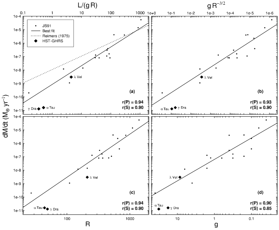
Figure 1: Mass loss rate for cool giant stars (JS91) is plotted against $L/(g\,R)$ (panel a), $g/R^{\frac{3}{2}}$ (b), $R$ (c), and $g$ (d). All quantities are given in solar units except for gravity which is in cgs units. The continuous lines represent least-squares fits to the data [eqs. (1)–(4)]. The Pearson and Spearman correlation coefficients are given. HST-GHRS results are also shown.

2.1 Mass Loss Formulae Revisited

As a first step in this project, we have undertaken a revision of all these formulae, employing the latest and most extensive dataset available in the literature—namely, that of JS91. The mass loss rates provided in JS91 were compared against more recent data (e.g., Guilain & Mauron 1996), and excellent agreement was found. If the distance adopted by JS91 lied more than about $2\sigma$ away from that based on Hipparcos trigonometric parallaxes, the star was discarded. Only five stars turned out to be discrepant, in a sample containing more than 20 giants. Employing ordinary least-squares regressions, we find that the following formulae provide adequate fits to the data (see also Fig. 1):

$$\frac{{\rm d}M}{{\rm d}t}=8.5\times 10^{-10}\left(\!\!\!\begin{array}[]{c}L\\ \overline{g\,R}\end{array}\!\!\!\right)^{+1.4}\,\,M_{\odot}\,{\rm yr}^{-1},$$ (1)

with $g$ in cgs units, and $L$ and $R$ in solar units. As can be seen, this represents a “generalized” form of Reimers’ original mass loss formula, essentially reproducing a later result by Reimers (1987). The exponent (+1.4) differs from the one in Reimers’ (1975) formula (+1.0) at $\approx 3\sigma$;

$$\frac{{\rm d}M}{{\rm d}t}=2.4\times 10^{-11}\left(\!\!\!\begin{array}[]{c}g\\ \overline{R^{\frac{3}{2}}}\end{array}\!\!\!\right)^{-0.9}\,\,M_{\odot}\,{\rm yr}^{-1},$$ (2)

likewise, but in the case of Mullan’s (1978) formula;

$$\frac{{\rm d}M}{{\rm d}t}=1.2\times 10^{-15}\,R^{+3.2}\,\,M_{\odot}\,{\rm yr}^{-1},$$ (3)

idem, Goldberg’s (1979) formula;

$$\frac{{\rm d}M}{{\rm d}t}=6.3\times 10^{-8}\,g^{-1.6}\,\,M_{\odot}\,{\rm yr}^{-1},$$ (4)

ibidem, JS91’s formula. In addition, the expression

$$\frac{{\rm d}M}{{\rm d}t}=3.4\times 10^{-12}\,L^{+1.1}\,g^{-0.9}\,\,M_{\odot}\,{\rm yr}^{-1},$$ (5)

suggested to us by D. VandenBerg, also provides a good fit to the data. “Occam’s razor” would favor equations (3) or (4) in comparison with the others, but otherwise we are unable to identify any of them as being obviously superior.

2.2 Caveats

We emphasize that mass loss formulae such as those given above should not be employed in astrophysical applications (stellar evolution, analysis of integrated galactic spectra, etc.) without keeping in mind these exceedingly important limitations:

1. As in Reimers’ (1975) case, equations (1) through (5) were derived based on Population I stars. Hence they too are not well established for low-metallicity stars. Moreover, there are only two first-ascent giants in the adopted sample;

2. Quoting Reimers (1977), “besides the basic [stellar] parameters $\ldots$ the mass-loss process is probably also influenced by the angular momentum, magnetic fields and close companions. The order of magnitude of such effects is completely unclear. Obviously, many observations will be necessary before we get a more detailed picture of stellar winds in red giants” (emphasis added). See also Dupree & Reimers (1987);

3. “One should always bear in mind that a simple $\ldots$ formula like that proposed can be expected to yield only correct order-of-magnitude results if extrapolated to the short-lived evolutionary phases near the tips of the giant branches” (Kudritzki & Reimers 1978);

4. “Most observations have been interpreted using models that are relatively simple (stationary, polytropic, spherically symmetric, homogeneous) and thus ‘observed’ mass loss rates or limits may be in error by orders of magnitude in some cases” (Willson 1999);

5. The two first-ascent giants analyzed by Robinson et al. (1998) using HST-GHRS, $\alpha$ Tau and $\gamma$ Dra, appear to both lie about one order of magnitude below the relations that best fit the JS91 data—two orders of magnitude in fact, if compared to Reimers’ formula (see Fig. 1). The K supergiant $\lambda$ Vel, analyzed by the same group (Mullan et al. 1998), appears in much better agreement with the adopted dataset and best fitting relations.

In effect, mass loss on the RGB is an excellent, but virtually untested, second-parameter candidate. It may be connected to GC density, rotational velocities, and abundance anomalies on the RGB. It will be extremely important to study mass loss in first-ascent, low-metallicity giants—in the field and in GCs alike—using the most adequate ground- and space-based facilities available, or expected to become available, in the course of the next decade. Moreover, in order to properly determine how (mean) mass loss behaves as a function of the fundamental physical parameters and metallicity, astrometric missions much more accurate than Hipparcos, such as SIM and GAIA, will certainly be necessary.

In the meantime, we suggest that using several different mass loss formulae (such as those provided in Sect. 2.1) constitutes a better approach than relying on a single one. This is the approach that we are going to follow in the rest of this paper.

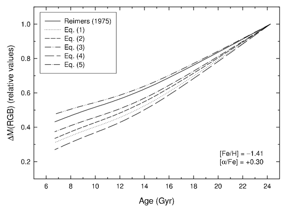
Figure 2: Dependence of mass loss on age, for the chemical composition indicated at the lower right-hand corner. For each mass loss formula, mass loss values were normalized to the highest value, attained at an age of 24.3 Gyr.

3 Implications for the Amount of Mass Lost by First-Ascent Giants

The latest RGB evolutionary tracks by VandenBerg et al. (2000) were employed in an investigation of the amount of mass lost on the RGB and its dependence on age. The effects of mass loss upon RGB evolution were ignored. In Figure 2, the mass loss–age relationship is shown for each of equations (1) through (5), and also for Reimers’ (1975) formula, for a metallicity ${\rm[Fe/H]}=-1.41$, $[\alpha/{\rm Fe}]=+0.30$. Even though the formulae from Section 2.1 are all based on the very same dataset, the implications differ from case to case.

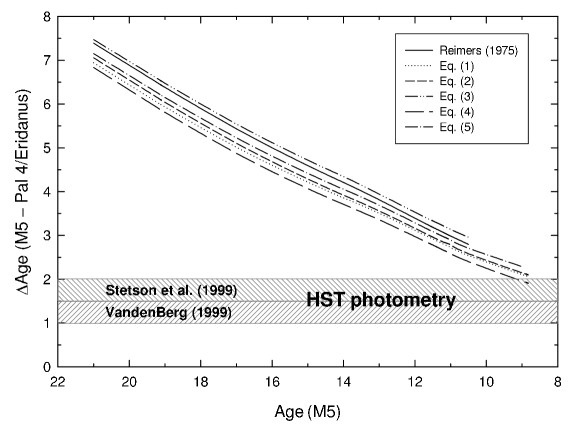
Figure 3: Difference in age (in Gyr) between M5 and Pal 4/Eridanus, derived for the several indicated mass loss formulae, as a function of the assumed M5 age (also in Gyr). The hatched areas correspond to the range in turnoff age differences between M5 and Pal 4/Eridanus, as estimated by Stetson et al. (1999) and VandenBerg (1999) from deep HST photometry.

4 The Second-Parameter Effect: the Case of Pal 4/Eridanus vs. M5

Stetson et al. (1999) presented $V$, $V-I$ color-magnitude diagrams for the outer-halo GCs Pal 4 and Eridanus, based on HST images. Analyzing their turnoff ages, they concluded that Pal 4 and Eridanus are younger than M5, a GC with similar metallicity but a bluer HB, by $1.5-2$ Gyr. Based on the same data, VandenBerg (1999) obtained a smaller age difference: $1-1.5$ Gyr. Are these values consistent with the relative HB types of Pal 4/Eridanus vs. M5?

To answer this question, we constructed detailed synthetic HB models (based on the evolutionary tracks described in Catelan et al. 1998) for M5 and Pal 4/Eridanus, thus obtaining the difference in mean HB mass between them—which was then transformed to a difference in age with the aid of the mass loss formulae from Section 2 and the RGB mass loss results from Section 3. Figure 3 shows the age difference thus obtained as a function of the adopted M5 age, in comparison with the turnoff determinations from Stetson et al. (1999) and VandenBerg (1999). Our assumed reddening values for Pal 4/Eridanus come from Schlegel et al. (1998); had the Harris (1996) values been adopted instead, the curves in Figure 3 corresponding to the different mass loss formulae would all be shifted upwards.

5 Conclusions

As one can see from Figure 3 our results indicate that, irrespective of the mass loss formula employed, age cannot be the only “second parameter” at play in the case of M5 vs. Pal 4/Eridanus, unless these GCs are younger than 10 Gyr.

References

Catelan M., Borissova J., Sweigart A.V., Spassova N., 1998, ApJ 494, 265

Catelan M., de Freitas Pacheco J.A., 1995, A&A 297, 345

Dupree A.K., Reimers D., 1987. In: Kondo Y., et al. (eds.) Exploring the Universe with the IUE Satellite. Dordrecht, Reidel, p. 321

Goldberg L., 1979, QJRAS 20, 361

Guilain Ch., Mauron N., 1996, A&A 314, 585

Harris W.E., 1996, AJ 112, 1487

Judge P.G., Stencel R.E., 1991, ApJ 371, 357 (JS91)

Kudritzki R.P., Reimers D., 1978, A&A 70, 227

Lee Y.-W., Demarque P., Zinn R., 1994, ApJ 423, 248

Mullan D.J., 1978, ApJ 226, 151

Mullan D.J., Carpenter K.G., Robinson R.D., 1998, ApJ 495, 927

Reimers D., 1975. In: Mémoires de la Societé Royale des Sciences de Liège, 6e serie, tome VIII, Problèmes D’Hydrodynamique Stellaire, p. 369

Reimers D., 1977, A&A 57, 395

Reimers D., 1987. In: Appenzeller I., Jordan C. (eds.) IAU Symp. 122, Circumstellar Matter. Dordrecht, Kluwer, p. 307

Robinson R.D., Carpenter K.G., Brown A., 1998, ApJ 503, 396

Rood R.T., Whitney J., D’Cruz N., 1997. In: Rood R.T., Renzini A. (eds.) Advances in Stellar Evolution. Cambridge, Cambridge University Press, p. 74

Schlegel D.J., Finkbeiner D.P., Davis M., 1998, ApJ 500, 525

VandenBerg D.A., 1999, ApJ, submitted

VandenBerg D.A., Swenson F.J., Rogers F.J., Iglesias C.A., Alexander D.R., 2000, ApJ 528, in press (January $20^{\rm th}$ issue)

Willson L.A., 1999. In: Livio M. (ed.) Unsolved Problems in Stellar Evolution. Cambridge, Cambridge University Press, p. 227