Plumes in stellar convection zones

Abstract

All numerical simulations of compressible convection reveal the presence of strong downwards directed flows. Thanks to helioseismology, such plumes have now been detected also at the top of the solar convection zone, on supergranular scales. Their properties may be crudely described by adopting Taylor’s turbulent entrainment hypothesis, whose validity is well established under various conditions. Using this model, one finds that the strong density stratification does not prevent the plumes from traversing the whole convection zone, and that they carry upwards a net energy flux. They penetrate to some extent in the adjacent stable region, where they establish an almost adiabatic stratification when there is little radiative diffusion. These plumes have a strong impact on the dynamics of stellar convection zones, and they play probably a key role in the dynamo mechanism.

Proceedings of the Fourteenth International Annual Florida Workshop in Nonlinear Astronomy and Physics, “Astrophysical Turbulence and Convection”  , University of Florida, Feb. 1999

(to appear in the Annals of the New York Academy of Sciences)

Département d’Astrophysique Stellaire et Galactique, Observatoire de Paris, Section Meudon, 92195 Meudon, France

1. Introduction

One of the main weaknesses of stellar physics remains our poor description of thermal convection. It is true that the widely used mixing-length treatment permits to construct models which represent fairly well the gross properties of stars, but it fails when one attempts to apply it to more subtle processes, such as convective penetration, the differential rotation of the Sun, or its magnetic activity.

The situation is rapidly changing however. Over the two past decades significant progress has been achieved through numerical simulations of increasingly ‘turbulent’ convection in a stratified medium. These have shown that fully compressible convection is highly intermittent, displaying strong, long-lived, downwards directed flows, which contrast with the slower, random upward motions (Hurlburt et al. 1986; Cattaneo et al. 1991; Nordlund et al. 1992; Muthsam et al. 1995; Singh et al. 1995; Brummel et al. 1996; Stein & Nordlund 1998). These coherent structures are called plumes (‘panaches’ in french), by analogy with those observed in the Earth atmosphere. They originate in the upper boundary layer, where they are initiated by the strong temperature and density fluctuations, which arise there in the steep superadiabatic gradient.

True, these numerical results are still difficult to apply as such to the convection zone of a star, because of the huge gap in the relevant control parameters, the Reynolds and the Prandtl numbers. But they suggest that coherent structures may play an important role in the dynamics of a turbulent convective layer, and thus open the possibility of a different description of stellar convection.

And indeed these plumes have now been detected in the upper layers of the solar convection zone, thanks to time-distance tomography. This powerful helioseismic technique reveals the presence of downdrafts apparently associated with the supergranular network, in which the temperature is strongly correlated with the vertical velocity (D’Silva et al. 1996; Duvall et al. 1997). Fig. 1 shows an example of such tomographies; it can been downloaded from the SOHO gallery on the Web.

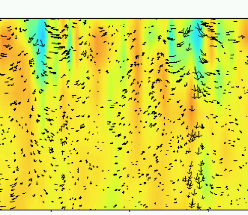
Figure 1.: Time-distance tomography with the MDI instrument on board of SOHO; the field shown measures 8 Mm in depth and 150 Mm in width. (http://sohowww.nascom.nasa.gov/gallery/MDI/mdi009.gif)

Turbulent plumes are commonly observed in the Earth atmosphere, where they rise above concentrated heat sources (chimneys, nuclear plants, volcanos, etc.). Their theoretical interpretation is still based on the entrainment hypothesis, which was first proposed by G.I. Taylor (cf. Morton et al. 1956); we recall it below. In astrophysics, plumes have been invoked by Schmitt et al. (1984) as responsible for the penetration into the stable domain beneath the solar convection zone. Somewhat later an estimate of that penetration has been given by Zahn (1991), which is also based on a crude plume model.

More recently, Rieutord and Zahn (1995) moved a step forwards, by letting the plumes develop through the whole convection zone. They adapted to a medium which is highly stratified, in density and temperature, the treatment which is used in geophysical fluid dynamics. Furthermore, they took into account the backflow which is induced by the confinement of the plumes in a limited volume, and which determines the depth the plumes may reach. This review recalls the main properties of that model; it will also address the role the plumes may play in convective penetration and in the generation of gravity waves.

2. One single plume in an isentropic stratification

We shall first examine the basic properties of a turbulent plume which resides in an isentropic, plane-parallel atmosphere, assuming that the plume is fed steadily by a cold layer of fluid lying on the top of the atmosphere. A schematic view of the flow in such a plume is given in fig. LABEL:plume.

Figure 2.: The plume flow in an adiabatic atmosphere (after Rieutord & Zahn 1995; courtesy A&A).

2.1. Governing equations

The equations governing the structure of turbulent plumes have been established in the original work of Morton et al. (1956). One assumes that the flow is stationary, that the plumes are axisymmetric about the vertical, and that all horizontal variations, namely those of the vertical velocity $v_{z}$, of the density excess $\delta\rho$ and of the excess of specific enthalpy $\delta h$, have the same gaussian profile:

$$\left\{\begin{array}[]{l}\displaystyle v_{z}(r,z)=V(z)\exp(-s^{2}/b^{2})\\ \displaystyle\delta\rho(r,z)=\Delta\rho(z)\exp(-s^{2}/b^{2})\\ \displaystyle\delta h(r,z)=\Delta h(z)\exp(-s^{2}/b^{2})\end{array}\right.$$ (1)

where $b\equiv b(z)$ is the effective radius of the plume. For convenience, we take the vertical coordinate $z$ pointing downward; the density and the specific enthalpy of the isentropic atmosphere will be designated by $\rho_{0}(z)$ and $h_{0}(z)$.

The equations describing the vertical profile of the plume are derived from the three basic equations of fluid mechanics expressing the conservation of mass, momentum and energy.

Conservation of mass.

In the steady flow of the plume, the mass conservation implies

$$\hbox{div}(\rho\vec{v})=\frac{1}{s}{\partial\over\partial s}\left({s\rho v_{s}}\right)+{\partial\over\partial z}\left({\rho v_{z}}\right)=0\ ;$$

when integrated over $s$, this equation becomes

$$\frac{d}{dz}\int_{0}^{+\infty}\!\rho v_{z}sds\;+\;[s\rho v_{s}]_{0}^{+\infty}=0.$$ (2)

The entrainment hypothesis made by G.I. Taylor postulates that the radial inflow of matter into the plume is proportional to the central vertical velocity:

$$\lim_{s\rightarrow+\infty}sv_{s}=-\alpha b(z)|v_{z}(0,z)|$$ (3)

where $\alpha$ is the entrainment constant. The absolute value guarantees that the plume is always accreting matter, whether it is directed upwards or downwards. Using the gaussian profile of $v_{z}$ and $\delta\rho$, one casts the mass equation in its final form

$$\frac{d}{dz}\left[\rho_{0}b^{2}V\right]=2\alpha\rho_{0}bV\,,$$ (4)

in the limit of vanishing density contrast $\Delta\rho/\rho_{0}\ll 1$.

Conservation of momentum.

Ignoring the viscous stresses, the flow obeys the steady Euler equation:

$$\partial_{j}(\rho v_{j}v_{i}+\delta p\,\delta_{ij})=\delta\!\rho\,g_{i}\,,$$

where the static equilibrium has been subtracted. We assume that the plume is in pressure balance with the surrounding medium; it leads us to

$$\frac{1}{s}{\partial\over\partial s}\left({s\rho v_{s}v_{z}}\right)+{\partial\over\partial z}\left({\rho v_{z}^{2}}\right)=\delta\!\rho\,g$$

($g$ is the gravity, which we assume constant). After integration as before, we get

$$\frac{d}{dz}\left[\rho_{0}b^{2}V^{2}\right]=2gb^{2}\Delta\rho\,.$$ (5)

Conservation of energy.

We start from the steady energy equation

$$\hbox{div}(\rho e\vec{v})=\hbox{div}(\chi\vec{\nabla}T)-p\hbox{div}\vec{v}\ ,$$

where $e$ is the specific internal energy and $\chi$ the radiative conductivity, and rewrite it by using the momentum equation and the definition of the specific enthalpy $dh\equiv de+d(p/\rho)$:

$$\hbox{div}\left[(h+{\frac{1}{2}}v^{2})\rho\vec{v}-\chi\vec{\nabla}T\right]=\rho\vec{v}\cdot{\vec{g}}.$$

This equation may be further simplified by remembering that

$${\vec{g}}=\vec{\nabla}h_{0}$$

in an isentropic atmosphere (see below). Finally, the conservation of the energy flux is expressed in conservative form:

$$\hbox{div}\left[\left(\delta h+{\frac{1}{2}}v^{2}\right)\rho\vec{v}-\chi\vec{\nabla}T\right]=0,$$ (6)

where we recognize respectively the enthalpy, kinetic and radiative fluxes.

To make contact with previous work, we first neglect the radiative flux. Proceeding as before, we integrate in the radial direction, and obtain

$${\frac{1}{2}}\rho_{0}b^{2}V\Delta h+\frac{1}{6}\rho_{0}b^{2}V^{3}=-F/\pi\ ,$$ (7)

where $F$ designates the total flux (enthalpy plus kinetic) carried by one plume.

From now on, we shall drop the subscript ₀, since there will be no ambiguity anymore between the local values of density and temperature, and their counterparts in the isentropic atmosphere.

Thermodynamics.

For simplicity, we shall assume that the fluid is a perfect monatomic gas, with $\gamma=5/3$ being the adiabatic exponent. We thus complete the system of governing equations with the two thermodynamic relations:

$$\Delta h=c_{p}\Delta T$$

$${\Delta\rho\over\rho}+{\Delta T\over T}=0$$

where the latter expresses the pressure balance between the plume and the surrounding medium ($c_{p}$ is the heat capacity at constant pressure).

The isentropic atmosphere.

As is well known, the isentropic atmosphere is a polytrope of index $q=1/(\gamma-1)$. In plane-parallel geometry, the density and the temperature vary with depth $z$ as:

$$\left\{\begin{array}[]{l}\displaystyle\rho(z)=\rho_{i}(z/z_{i})^{q}\\ \\ \displaystyle T(z)=T_{i}(z/z_{i}).\end{array}\right.$$ (8)

The origin of the vertical coordinate $z$ is taken at the ‘surface’, where pressure, density and temperature all vanish, and the subscript _i designates the reference level for which we choose here the base of the atmosphere. The reference temperature $T_{i}$ is related to the reference depth by $z_{i}=c_{p}T_{i}/g$.

2.2. Asymptotic behavior

The equations governing the plume flow are nonlinear and in most cases it is necessary to integrate them numerically, with boundary conditions imposed at the start of the plume, for instance on $\Delta\rho$, $b$ and $V$. However, the system has asymptotic solutions which can easily be obtained in analytic form. The one which presents most interest corresponds to the developed phase of the downwards directed plume, when it is fully controlled by entrainment. The solution then obeys the power laws

$$b=b_{i}\left({z/z_{i}}\right)^{p},\quad V=V_{i}\left({z/z_{i}}\right)^{r},\quad\Delta\rho=\Delta\rho_{i}\left({z/z_{i}}\right)^{m}$$ (9)

where the exponents take the values:

$$\left\{\begin{array}[]{l}p=1\\ \\ \displaystyle r=-\frac{q+2}{3}=-\frac{2\gamma-1}{3(\gamma-1)}\\ \\ \displaystyle m=-\frac{2q+7}{3}=-\frac{7\gamma-5}{3(\gamma-1)}\,.\end{array}\right.$$ (10)

A direct consequence of Taylor’s entrainment hypothesis (3) is that the plume radius increases linearly with depth. The half-angle $\beta=$atan$(b_{i}/z_{i})$ of the cone is related to the adiabatic exponent:

$$\tan\beta=\frac{3\alpha}{q+2}=\frac{3\alpha(\gamma-1)}{2\gamma-1}\,.$$ (11)

With $\gamma=5/3$ (perfect monatomic gas), we have $\tan\beta=6\alpha/7$, whereas $\tan\beta=6\alpha/5$ in the absence of stratification. The entrainment coefficient $\alpha$ has been determined experimentally in various situations, and the value 0.083 is widely adopted (Turner 1986); we shall assume that this value also applies to our fully ionized gas.

For given initial conditions imposed at the top of the plume, the solutions rapidly reach their asymptotic regime: the plumes start contracting while they accelerate, and then they take their characteristic conical shape (cf. Rieutord & Zahn 1995).

Note that one does not retrieve the incompressible case by letting the polytropic index tend to zero, $q\rightarrow 0$. The reason for this singular limit is the assumption made in the classical treatment (Morton et al. 1956) that the surrounding medium is isothermal, while in our stratified atmosphere the temperature grows linearly with depth. Let us emphasize however that our asymptotic solution (9) is rather special, since its focal point $z=0$ coincides with the ‘surface’ of the atmosphere.

2.3. Turbulent plumes carry upwards a net energy flux

An interesting property of this asymptotic regime is the strict proportionality between the flux of kinetic energy and that of enthalpy:

$$R=\frac{\displaystyle\int{\frac{1}{2}}\rho V^{3}sds}{\displaystyle\int\rho c_{p}\,\delta T\,Vsds}=cst.$$ (12)

With the gaussian profile we have adopted for the plume, this ratio is given by

$$R=-\frac{2}{q+2}=-\frac{2\gamma-2}{2\gamma-1}\;.$$ (13)

Its value is 1 for the Boussinesq fluid (no density stratification) but it is 4/7 in the isentropic atmosphere (for the perfect monatomic gas), meaning that the net energy flux is directed upwards.

In their numerical experiment Cattaneo et al. (1991) observed to their surprise that the strong downdrafts transported a flux of kinetic energy which very nearly canceled the flux of enthalpy. The reason is that their plumes were not turbulent, but laminar flows which satisfied approximately Bernoulli’s theorem. In recent simulations, which have been achieved with better spatial resolution, there is more entrainment, and the plumes do carry a net energy flux upwards.

3. Towards a more realistic model; application to the solar convection zone

Up to now, we have considered the case of a single plume in an unlimited isentropic plane layer. To progress towards a more realistic situation, we must take into account the spherical geometry of the fluid layer and include the variations of gravity with depth. Here we shall apply the model to the solar convection zone (SCZ); the convective core with its rising plumes has been treated by Lo and Schatzman (1997).

We neglect the mass of the envelope, so that the density and temperature field of the background are given by

$$\left\{\begin{array}[]{l}\displaystyle T(z)=T_{i}\;\frac{\eta}{1-\eta}\left(\frac{1}{x}-1\right)\\ \\ \displaystyle\rho(z)=\rho_{i}\left({T(z)\over T_{i}}\right)^{q}\\ \\ \displaystyle x=1-z\end{array}\right.$$ (14)

where $x=r/R_{\odot}$ is the radial coordinate scaled by the radius, and $\eta=r_{\rm cz}/R_{\odot}$ its value at the base of the SCZ (our reference level).

We shall also take into account the radiative flux in the energy equation, thus (7) now reads

$${\frac{1}{2}}\rho b^{2}V\Delta h+\frac{1}{6}\rho b^{2}V^{3}=-(F_{\rm tot}-F_{\rm rad})/\pi\ .$$ (15)

With our assumption that all the convective energy is transported by the plumes, whose number is $N$, the total flux amounts to the luminosity of the star:

$$N\,F_{\rm tot}=L_{\odot}.$$ (16)

The radiative contribution to the flux carried by one plume is $F_{\rm rad}$, where

$$N\,F_{\rm rad}=L_{\rm rad}=-4\pi r^{2}\,\chi\left(\frac{\partial T}{\partial z}\right)_{\rm ad},\quad\chi=\frac{16\sigma T^{3}}{3\kappa\rho}\,,$$

with $\chi$ being the radiative conductivity, $\kappa$ the opacity, and $\sigma$ the Stefan constant.

3.1. Plumes diving in a rising counterflow

We shall now take into account that there are numerous plumes and that they share a finite volume. This has two consequences: the plumes will interact and possibly merge, and they will move in a rising counterflow. Let us first estimate the maximum number of plumes which may coexist in the SCZ, assuming that they all originate at the top and that all reach its bottom without being hindered by the counterflow. This number is given by the ratio of the area of the base of the SCZ to the section of a single plume at this depth:

$$N=4\left[{\eta\over(1-\eta)\tan\beta}\right]^{2}$$

where $\beta$ is given by (11), and $\eta=r_{\rm cz}/R_{\odot}$ is the scaled radius of the base of the SCZ. Taking $\eta=0.7$, the result is $N_{\rm max}\sim 4300$. We see that even if the plumes were closely packed, they would not be very numerous. But they will be actually less, because as soon as their occupy more than half of the total area, at depth $z_{i}/\sqrt{2}$, the velocity of the backflow exceeds that of the plumes, and this will affect their dynamics.

To model the effect of this counterflow, we shall assume that the entrainment of mass into the plume is proportional to the relative velocity of the plume with respect to the surrounding fluid. This yields the mass conservation equation

$$\frac{d}{dz}\left[\rho b^{2}V\right]=2\alpha\,\rho b(V-V_{u})$$ (17)

where $V_{u}$ is the upward velocity of the surrounding fluid; since $V_{u}<0$, entrainment is enhanced. The momentum equation needs also be completed by a term taking into account the entrainment of momentum into the plume. We thus transform (5) into

$$\frac{d}{dz}\left[\rho b^{2}V^{2}\right]=2gb^{2}\Delta\rho+4\alpha\,\rho bV_{u}(V-V_{u})\,.$$ (18)

Equations (17) and (18) are completed by

$$(4\pi r^{2}-N\pi b^{2})\rho V_{u}+N\pi b^{2}\rho V=0$$ (19)

which expresses the global conservation of mass. The consequence of these additional effects is that plumes are able to reach the bottom of the convection zone only if they are strong enough, and not too numerous. From the numerical integration of these equations it turns out that only about $1000$ plumes are able to reach the bottom of the SCZ (see Rieutord & Zahn 1995).

3.2. Plume coalescence

At the top of the SCZ, the number of plumes is probably of the same order as that of the granules, which is considerably larger than 1000. Hence a drastic reduction of the plumes number must occur as depth increases. The plumes are stopped at a level which depends on their strength: only the 1000 strongest are able to reach the bottom. The others will either dissolve in the (turbulent) backflow and disappear as such, or they will merge with a stronger companion.

Such merging is observed in the numerical simulations (Stein & Nordlund 1989; Spruit et al. 1990): two neighboring plumes are advected by each other, since they both accrete surrounding fluid, and they are pulled to each other until they finally coalesce. The merging depth can be estimated by assuming the flow be in the asymptotic regime; the result is

$$z_{m}=\frac{d}{\sqrt{2\alpha\beta}}$$ (20)

where $d$ is the initial separation of the two plumes, which we assumed here to be identical. Using the value of $\beta$ for the monatomic ideal gas and $\alpha=0.083$, we get $z_{m}\sim 9.2\,d\ .$

Similar coalescences will then repeat at increasing depths, until the survivors reach the base of the convection zone, in a sort of inverse cascade with a large scale flow building up from smaller scales.

4. Penetration at the base of a convection zone

When the plumes reach the bottom of the unstable domain, they still possess a finite velocity which enables them to penetrate some distance into the stable, subadiabatic region, where they establish a nearly adiabatic stratification by releasing their entropy when they come to rest. A first attempt to estimate the extent of penetration of such plumes was made by Schmitt et al. (1984). However, they did not include the return flow, and they had to impose both the velocity $V$ and the filling factor $f$ at the base of the unstable domain because they did not solve the plume equations above that level. They found empirically that the penetration depth varies as $f^{1/2}V^{3/2}$, and this scaling can be easily explained.

Figure 3.: Schematic structure of the base of a convective envelope (after Zahn 1991; courtesy A&A).

4.1. An estimate of the penetration penetration depth

The stratification at the base of the a convective envelope is sketched in fig. (3). (A) designates the unstable region, where the temperature gradient is maintained close to adiabatic by the convective motions. One thus assumes that the radiative leaks are negligible compared to the advective transport of heat, which is the case when the Péclet number is much larger than unity:

$$Pec={v\ell\over K}\gg 1,\quad K={\chi\over\rho c_{p}},$$ (21)

where $K$ is the thermal diffusivity and $\chi$ the radiative conductivity. $v$ and $\ell$ are the velocity and size characterizing the convective motions, i.e. here the central velocity $V$ and the width $b$ of our plumes. At the base of the SCZ, $Pec\approx 10^{6}$.

Due to the steady increase with depth of the radiative conductivity $\chi$, the radiative flux $F_{\rm rad}=\chi(dT/dz)_{\rm ad}$ rises until it equals the total flux $F_{\rm total}$ at the level $z=z_{i}$, where also the radiative gradient equals the adiabatic gradient: $(dT/dz)_{\rm rad}=(dT/dz)_{\rm ad}$. If there were no convective penetration, this would be the edge of the convection zone, as predicted by the Schwarzschild criterion, and the temperature gradient would thereafter decrease as $dT/dz=F_{\rm total}/\chi$. But the motions penetrate into the stable region (B) and they render it nearly adiabatic over some distance $d_{\rm pen}$, while being decelerated by the buoyancy force. When the Péclet number has dropped below unity, the temperature gradient settles from adiabatic to radiative in a thermal boundary layer (C).

Since the penetration depth is rather small, one may simplify the problem by ignoring the variation with depth of most quantities (density, width of the plume, etc.), and by neglecting the kinetic energy flux and the turbulent entrainment (or detrainment). One keeps of course the variation with $z$ of the conductivity; in the vicinity of $z_{i}$, the radiative flux is approximated by

$$F_{\rm rad}=\chi\left({dT\over dz}\right)_{\rm ad}=F_{\rm total}\left[1+\left({d\chi\over dz}\right)_{i}\left(z-z_{i}\right)\right]\,.$$ (22)

Therefore the convective flux varies as

$$F_{\rm conv}=-F_{\rm total}\left({d\chi\over dz}\right)_{i}\left(z-z_{i}\right)\,.$$ (23)

This enthalpy flux may be expressed in terms of the vertical velocity and of the temperature contrast in the plumes, as in (7):

$$F_{\rm conv}=-f\rho c_{p}V\Delta T\,,$$ (24)

where we have introduced the filling factor $f$ of the plumes, defined as the fractional area covered by them: $f=Nb^{2}/R^{2}_{\rm cz}$.

To estimate the penetration depth, we follow the plumes from $z=z_{i}$, where their velocity is $V_{i}$, until they stop at $z=z_{i}+d_{\rm pen}$. Their deceleration is described to first order by

$${1\over 2}{dV^{2}\over dz}=g{\Delta\rho\over\rho}=-g{\Delta T\over T}.$$ (25)

After elimination of $\Delta T$ with (24), the integration of (25) yields the following expression for the penetration depth $d_{\rm pen}$:

$$d_{\rm pen}^{2}={3\over 5}H_{p}H_{\chi}\left\{f{\rho V_{i}^{3}\over F_{\rm total}}\right\}={3\over 5}H_{p}H_{\chi}Q\,,$$ (26)

where $H_{p}$ is the scale-height of the pressure and $H_{\chi}$ that of the radiative conductivity. This is the scaling obtained empirically by Schmitt et al. (1984).

At that point one may argue that the term $Q$ in curly brackets is determined by the dynamics in the convection zone, and that it will not depend much on its depth, provided this depth is large enough and that convection is sufficiently adiabatic. $Q$ is probably smaller than unity: in the mixing length treatment, $Q=(1/10)\,\Lambda/H_{p}$ in the bulk of the convection zone. This figure, with $\Lambda/H_{p}\approx 1.5$ and $H_{\chi}\approx H_{p}/2$, would yield a penetration depth of the order of $1/5$ of the pressure scale-height at the base of the solar convection zone.

4.2. Penetration of plumes originating at the top of the convection zone

Rieutord and Zahn (1995) computed the penetration in a more consistent way, by integrating the governing equations from the top of the convection zone until the plumes come to rest. When neglecting the backflow, the penetration extends to about one half of the pressure scale-height, independent on the number of plumes. But the picture changes drastically when one includes the interaction of the plumes with the backflow. Then the penetration depth depends on the number of plumes: it decreases almost linearly with $N$, from one pressure scale-height for $N\rightarrow 0$ to $0$ for $N\approx 1200$. The reason for this trend is that the backflow increases with the number of plumes, and that it slows down their motion by loading them with upward momentum.

Unfortunately, this model is unable to predict the number of plumes. Moreover, a much more sophisticated model is needed to describe the termination of the plume flow, which would include the loss of mass by the plume in this region, or ‘detrainment’, and its transfer to the upward motion.

4.3. Penetration vs. overshooting

What we have called convective penetration is that part of the excursion of convective motions into the stable region below where they enforce an almost adiabatic stratification ($\nabla_{\rm ad}-\nabla\ll 1$). It corresponds to region (B) in fig. 3, in which the Péclet number is substantially larger than unity (we recall that at the base of the SCZ, $Pec\approx 10^{6}$). In comparison, the thermal adjustment layer (C) is very thin: about 1 km in the Sun, assuming that all plumes have the same strength (Zahn 1991).

The situation is very different in stars which possess a shallow convection zone. For instance, at the base of the convection zone of an A-type star, $Pec\approx 1/100$, which means that the convective motions which enter the stable layer below rapidly settle in thermal equilibrium with their surroundings, and that they hardly feel the buoyancy force (Toomre et al. 1976; Freytag et al. 1996). The region (B) has disappeared – all what remains is region (C). To insist on the contrast with the almost adiabatic penetration at high Péclet number, we prefer to call this convective overshoot (or undershoot).

This is not only semantic matter. To take one example, numerical simulations which are performed to represent A-type stars cannot be used to predict the amount of penetration below the solar convection zone, as was attempted by Blöcker et al. (1998). In fact, for lack of spatial resolution, present day simulations are unable to achieve a Péclet number which would realistically describe convective penetration; for instance, in the calculations made by Hurlburt et al. (1994), regions (B) and (C) are of comparable size, and a substantial fraction of the extension into the stable region is due to overshoot.

4.4. Generation of internal gravity waves

In the laboratory, convective penetration is observed to generate internal waves, which propagate in the stable adjacent layer (Townsend 1966; Adrian 1975). the same is also expected at the boundary of stellar convection zones. Such waves have indeed been observed in numerical simulations of penetrative convection, where they seem to be produced by the pronounced downdrafts (Hurlburt et al. 1986; Hurlburt et al. 1994), which are the 2-dimensional analogues of 3-dimensional plumes. In these calculations one observes a strong feedback of the waves on the downdrafts, because the waves are reflected back by the lower boundary of the computational domain, a property which is not expected from the solar gravity waves produced by the plumes.

The generation of gravity waves by turbulent plumes is presently being investigated by M. Kiraga, in 2- and 3-dimensional simulations. He takes great care of avoiding the reflexion of the waves by the lower boundary of his computational domain, by implementing in its vicinity a strong viscous damping. The first results have been presented at the Granada workshop on convection (Kiraga et al. 1999); they look promising, and will be used to test the prescriptions which have been proposed for estimating the flux of gravity waves.

Our interest in these gravity waves is motivated by the fact that they may extract angular momentum from the radiative interior of solar-type stars (see Kumar & Quataert 1997; Zahn et al. 1997; Kumar et al. 1999).

5. Summarizing the properties of turbulent plumes

There is little doubt that the convection zone of solar-like stars exhibits strong spatial intermittency, with downwards directed plumes carrying a substantial fraction of the energy flux. Such plumes are seen in all numerical simulations, and they have now been observed in the uppermost part of the solar convection zone.

If Taylor’s parametrization of the entrainment of surrounding fluid into turbulent plumes holds in the hot plasma of stellar interiors, and we see no reason why it should not, then we expect such plumes to traverse the whole convection zone. According to the crude model presented above in §2, these plumes behave much as if they were traversing an isentropic atmosphere, with no feed-back at all, and ignoring the radiation flux. Shortly after their start, they reach an asymptotic regime with their size increasing linearly with depth. Due to the density stratification, the cone angle $\beta$ is somewhat smaller than in the Boussinesq case treated so far: $\tan\beta=6\alpha/7$ instead of $6\alpha/5$, with $\alpha$ being the entrainment constant.

These plumes carry kinetic energy downwards, i.e. in the ‘wrong’ direction. But their enthalpy flux always exceeds the kinetic flux: the ratio between the two is constant in the asymptotic regime, and its value is 4/7, if one assumes that the horizontal profile of the plume is gaussian.

The maximum number of plumes that may reach the base of the solar convection zone, when taking the counterflow into account, is around 1000, which means that the spacing between plumes is about 60 Mm. Note however that this evaluation is based on a very strong assumption: namely that the totality of the convective energy flux (enthalpy plus kinetic) is carried by the plumes, thus neglecting the contribution of the interstitial medium.

Finally, under the same assumption, the extent of penetration, at the base of the convection zone, depends on the number of plumes $N$ reaching that level: it varies from $0$ for $N\approx 12000$ to one pressure scale-height for $N\rightarrow 0$. Unfortunately, the number of plumes cannot be predicted with the simple model presented above. Let us recall that helioseismology yields a value of about $0.1H_{p}$, with the assumption that there is sharp transition from adiabatic to radiative slope at the edge of the penetration layer (Roxburgh & Vorontsov 1994). With plumes of different strength, the transition would be smoother and more difficult to diagnostic.

All these results are independent of the top boundary conditions on the mass flux and on the initial momentum flux carried by the plumes. What determines the flow is the convective energy flux near the surface, which would be conserved along the plume if there were no radiative transport. Unfortunately the simple model presented above is unable to render the complex dynamics of these layers, where important radiative exchanges occur. They can only been described by full-fledged 3-dimensional hydrodynamical simulations, such as performed by Å. Nordlund, R. Stein and their collaborators. However we cannot rule out that a sophisticated closure model, well beyond what has been described above, may succeed in better capturing the main properties of such turbulent plumes (see V. Canuto’s contribution to this workshop).

How do these plumes change our picture of stellar convection zones? Plumes presumably exert an important effect on the thermal structure – that is, on the small deviations from the isentropic stratification which are known to induce meridional circulation. The reason for this is that the heat transport by the plumes is of advective nature, whereas in most models so far, as for example in the mixing-length treatment, it has been represented by a diffusive process.

They will also play a major role in the dynamics of a convection zone, and in determining its rotation profile. Since the ambiant angular momentum will be entrained into the plumes, these will spin up with depth, and they will concentrate both vorticity and helicity. Owing to their robustness, such vortices could well be the cause of the observed differential rotation, especially of its peculiar property of being quasi-independent of depth (Brown et al. 1989; Kosovichev et al. 1997).

Furthermore, one can easily imagine that plumes play a major role in the generation and in the confinement of magnetic fields. Since they are sites of high helicity, they will be the seat of strong alpha-effect. The dynamo simulations of Brandenburg et al. (1996) have shown that laminar diving plumes are indeed playing an important part in the field generation and its storage at the base of the convective layer. In more recent simulations, they have been clearly observed to ‘pump down’ the magnetic field, which is definitely an advective process (Dorch 1998).

To conclude, we have yet to assess all the consequences of the presence of plumes in stellar convection zones. For that we have to rely mainly on numerical simulations, since the stratification is much stronger in stars than in the Earth atmosphere, and since it cannot be reproduced in the laboratory. These simulations have not reached yet a sufficient resolution to adequately describe turbulent plumes, but they are progressing at fast pace, and their results can be checked through helioseismology.

References

Adrian, R. J., 1975, J. Fluid Mech. 69, 753

Blöcker, T., H. Holweger, B. Freytag, F. Herwig, H.-G. Ludwig & M. Steffen, 1998, Space Sci. Rev. 85, 105

Brandenburg, A., R. L. Jennings, Å. Nordlund, M. Rieutord, R. F. Stein & I. Tuominen, 1996, J. Fluid Mech. 306, 325

Brown, T., J. Christensen-Dalsgaard, W. Dziembowski, P. Goode & C. Morrow, 1989, ApJ 343, 526

Brummell, N. H., N. E. Hurlburt & J. Toomre, 1996, ApJ 473, 494

Cattaneo, F., N. Brummell, J. Toomre, A. Malagoli & N. E. Hurlburt, 1991, ApJ 370, 282

Dorch, S. B., 1998, PhD thesis (http://www.astro.ku.dk/~dorch/thesis/)

Duvall, T. Jr., A. G. Kosovichev & P. H. Scherrer, 1998, Proc. IAU Symp. 181 ‘Sounding solar and stellar interiors’ (ed. J. Provost & F.-X. Schmider; Dordrecht Kluwer Acad. Publ.), 83

Duvall, T. Jr., A. G. Kosovichev, et al., 1997, Solar Phys. 170, 63

D’Silva, S., J. T. Jr. Duvall, S. M. Jefferies & J. W. Harvey, 1996, ApJ 471, 1030

Freytag B., H.-G. Ludwig & M. Steffen, 1996, A&A 313, 497

Hurlburt, N. E., J. Toomre & J. M. Massaguer, 1986, ApJ 311, 563

Hurlburt, N. E., J. Toomre, J. M. Massaguer & J.-P. Zahn, 1994, ApJ 421, 245

Kiraga, M., J.-P. Zahn, K. Stȩpień, K. Jahn, M. Rózyczka & H. J. Muthsam, 1999, Proc. Granada workshop on ‘Theory and tests of convection in stellar structure’; PASP Conf. Ser. 173 (in press)

Kosovichev, A. G. et al., 1997, Solar Phys. 170, 43

Kumar P. & E. J. Quataert, 1997, ApJ 479, L51

Kumar P., S. Talon & J.-P. Zahn, 1999, ApJ 520, 859

Lo, Y.-C. & E. Schatzman, 1997, A&A 322, 545

Morton, B., G. I. Taylor & J. Turner, 1956, Proc. Roy. Soc. London 234, 1

Muthsam, H. J., W. Göb, F. Kupka, W. Liebich & J. Zöchling, 1995, A&A 293, 127

Nordlund, Å., A. Brandenburg, R. Jennings, M. Rieutord, J. Ruokolainen, R. F. Stein & I. Tuominen, 1992, ApJ 392, 647

Rieutord, M. & J.-P. Zahn, 1995, A&A 296, 127

Roxburgh, I. W. & S. V. Vorontsov, 1994, MNRAS 520, 859

Schmitt, J., R. Rosner & H. Bohn, 1984, ApJ 282, 316

Singh, H. P., I. W. Roxburgh & K. L. Chan, 1995, A&A 295, 703

Singh, H. P., I. W. Roxburgh & K. L. Chan, 1998, A&A 340, 178

Spruit, H., Å. Nordlund & A. M. Title, 1990, Ann. Rev. A&A 28, 263

Stein, R. F. & Å. Nordlund, 1989, ApJ 342, L95

Stein, R. F. & Å. Nordlund, 1998, ApJ 499, 914

Toomre, J., J.-P. Zahn, J. Latour & E. A. Spiegel, 1976, ApJ 207, 545

Townsend, A. A., 1966, Quart. J. Roy. Met. Soc. 90, 248

Turner, J. S., 1986, J. Fluid Mech. 173, 431

Zahn, J.-P., 1991, A&A 252, 179

Zahn, J.-P., S. Talon & J. Matias, 1997, ApJ 322, 320