Period–Luminosity–Colour distribution and classification of Galactic oxygen–rich LPVs

Abstract

The absolute $K$ magnitudes and kinematic parameters of about 350 oxygen–rich Long–Period Variable stars are calibrated, by means of an up–to–date maximum–likelihood method, using Hipparcos parallaxes and proper motions together with radial velocities and, as additional data, periods and $V-K$ colour indices. Four groups, differing by their kinematics and mean magnitudes, are found. For each of them, we also obtain the distributions of magnitude, period and de-reddened colour of the base population, as well as de-biased period–luminosity–colour relations and their two–dimensional projections. The SRa semiregulars do not seem to constitute a separate class of LPVs. The SRb appear to belong to two populations of different ages. In a PL diagram, they constitute two evolutionary sequences towards the Mira stage. The Miras of the disk appear to pulsate on a lower–order mode. The slopes of their de-biased PL and PC relations are found to be very different from the ones of the Oxygen Miras of the LMC. This suggests that a significant number of so–called Miras of the LMC are misclassified. This also suggests that the Miras of the LMC do not constitute a homogeneous group, but include a significant proportion of metal–deficient stars, suggesting a relatively smooth star formation history. As a consequence, one may not trivially transpose the LMC period–luminosity relation from one galaxy to the other.

1 Introduction

The Hipparcos satellite has provided high–precision parallaxes and proper motions of a relatively large number of Long–Period Variable stars (LPV) in the solar neighbourhood. In this paper and in the next ones (Barthès & Luri bl99 (1999), Barthès et al. bla99 (1999), hereafter Papers II and III), which only concern those LPVs belonging to the Asymptotic Giant Branch (i.e. Mira, SRa and SRb stars), the Hipparcos data are exploited, together with radial velocities, $K$ magnitudes, periods, as well as $V-K$ and $J-K$ colour indices, by using a specifically adapted maximum–likelihood method of luminosity calibration. We obtain model distributions of absolute magnitude, dereddened colours and period of several groups of stars. We derive de-biased relations between the period, the absolute magnitude and the colour indices (PLC relations).

In this paper, the statistical model makes use of the $V-K$ colour index. The $J-K$ index is used only a posteriori in order to check the reliability of the results. In paper II, the results will be confronted with theoretical models of LPV pulsation. In paper III, a similar work will be performed with $J-K$ included in the statistical model.

In the next section, the calibration method is presented. The data are detailed in Sect. 3. The results of the luminosity calibration are given in Sect. 4. Their consequences in terms of PLC, PL, PC and LC relations are given and commented in Sect. 5 (these relations concern the sample when they involve the $J-K$ index, and the population in all other cases). Then, Sect. 6 summarizes and concludes this paper.

2 Calibration method

This work is based on the LM method, which has been designed to fully exploit the Hipparcos data to obtain luminosity calibrations. The mathematical foundation of this method was presented in Luri (luri95 (1995)) and Luri, Mennessier et al. (1996a ). Its main characteristics are:

• It is based on a maximum–likelihood algorithm;

• It is able to use all the available information on the stars: apparent magnitude, galactic coordinates, trigonometric parallax, proper motions, radial velocity and other relevant parameters (photometry, metallicity, period, etc.), and takes into account, as an additional constraint, the existence of mean relations between, e.g., period, luminosity and colour, whose analytical form is given a priori;

• It allows a detailed modelling of the kinematics, the spatial distribution, and also the distribution of luminosity, period and colour of the sample.

  In the implementation presented in this paper, the stars are assumed to be exponentially distributed about the galactic plane and their velocities to follow a Schwarzschild ellipsoid. The period and colour are assumed to follow a bivariate normal distribution, including a correlation between the two variables. This generates elliptic iso–probability contours in the period–colour plane. For each given combination of period and colour, the individual absolute magnitudes of the stars are assumed to be normal–distributed about the mean value given by a period–luminosity–colour relation, e.g. $M_{K}=A\,\log P\,+\,B\,(V-K)_{0}\,+\,C$. The resulting 3D distribution looks like a flattened ellipsoid whose main symmetry plane is the PLC relation. All parameters of the model are determined by maximum–likelihood estimation;

• The method takes into account the observational selection criteria that were used when making the sample — this is very important for obtaining unbiased results (Brown et al. brown97 (1997));

• It takes into account the effects of the observational errors; the results are not biased by them and even low–accuracy data (which would otherwise be useless) can be included;

• The galactic rotation is taken into account by introducing in the model an Oort–Lindblad first–order differential rotation with $A_{0}=14.4$, $B_{0}=-12.8\,\,{\rm km}.{\rm s}^{-1}.{\rm kpc}^{-1}$ and $R_{\rm sun}=8.5$ kpc;

• The interstellar absorption is taken into account, using the 3D model of Arenou et al. (arenou92 (1992)).

A further important feature of the LM method is its capability to separate and characterize, in the sample, groups of stars with different properties (e.g. luminosity, kinematics, spatial distribution…). The number of groups has to be fixed beforehand (see Sect. 4 for criteria). Then, separate results are obtained for each group, and this provides a much more meaningful information than a global result for the mixture of all of them would.

For the population corresponding to each identified group, the LM method provides unbiased estimates of the model parameters, i.e. for the version used in this study:

• The parameters of the absolute magnitude distribution, i.e. the coefficients of the mean period–luminosity–colour relation, and the dispersion around it ($\sigma_{M}$);

• The velocity distribution: mean velocities $(U_{0},V_{0},W_{0})$ and dispersions $(\sigma_{U},\sigma_{V},\sigma_{W})$;

• The spatial distribution: the scale heigth $Z_{0}$;

• The period–colour index distribution: mean of the logarithm of the period $\overline{\log P}$, mean de-reddened colour index, e.g. $\overline{(V-K)_{0}}$, the associated dispersions $\sigma_{\log P}$ and, e.g., $\sigma_{(V-K)_{0}}$, and the correlation between log period and colour;

• The percentage of the sample in each group: %.

In addition, the parameters of the selection function generating the sample are obtained for each group.

The LM method also yields improved individual distance estimates (and thus improved absolute magnitude estimates) which take into account all the available information on each star: the trigonometric parallax $\pi_{t}$ and other measurements (magnitude, $\alpha$, $\delta$, $\mu_{\alpha}$, $\mu_{\delta}$, $v_{r}$, $P$, colour). This estimation is free of any bias due to observational selection or observational errors, because both are taken into account by the method.

3 Data and other a priori information

3.1 Sampling

Our sample is made of the 154 Miras and 203 Semiregulars (34 SRa and 169 SRb) belonging to the Hipparcos Catalogue and for which mean values of both $V$ and $K$ magnitudes could be estimated. Their list is given in the Appendix B. For 257 stars, $J$ was available too.

The selection of the LPVs to be included in the Hipparcos Input Catalogue (Mennessier & Baglin mom88 (1988)), and thus to be observed by the satellite, was based on the General Catalogue of Variable Stars [GCVS] (Kholopov et al. gcvs85 (1985), 1987) and on a criterium of visibility: only those stars that were visible (i.e. with an apparent magnitude below the Hipparcos magnitude limit, $m<m_{lim}$) more than 80 % of the time were included in the observation programme. This condition can be written as:

$$\frac{m_{lim}-m_{max}}{m_{min}-m_{max}}>0.8\,,$$

translating into a linear relationship $m_{min}<a+b\;m_{max}$. On the other hand, the amplitudes of the LPV stars lie within a certain range $A_{min}\leq A\leq A_{max}$. One can easily see in Fig. 1 that, with these criteria, all LPVs up to a certain magnitude $m_{c}$ are selected and then, from $m_{c}$ up to a limiting magnitude $m_{lim}^{\prime}$, the probability of selecting a star decreases linearly.

As said above, within the frame of the Hipparcos Catalogue, our sample only includes stars for which mean values of both $V$ and $K$ could be obtained. Thus, in any case, the only relevant selection effects (within the general frame of the GCVS) are related to the apparent magnitudes of the stars. In order to account for these combined effects, a selection function $S(m)$ was introduced into the statistical model. Consistently with Fig. 1, it was defined so that all stars are selected up to a magnitude ${\mathfrak{m}}_{\mathfrak{c}}$ and then, up to a limiting magnitude ${\mathfrak{m}}_{\mathfrak{lim}}^{\prime}$, the number of selected stars linearly decreases. The value of ${\mathfrak{m}}_{\mathfrak{lim}}^{\prime}$ was taken equal to the apparent magnitude of the faintest star of the sample, and ${\mathfrak{m}}_{\mathfrak{c}}$ is determined (together with all other free parameters) by the LM method. In this way, the selection function adapts itself to the sample (and to each group that it contains, if several populations are assumed).

One must however remember that, despite the relatively large magnitude limit of the GCVS ($V\simeq 15$, to be compared to the Hipparcos limit $\simeq 13$), the sample of Mira, SRa and SRb stars found therein is not necessarily complete at much lower magnitudes. Indeed, in case of poor data (a frequent problem with Semiregulars, according to Lebzelter et al. [lebz95 (1995)]), it is difficult to detect the variability and to evaluate the amplitude and irregularity of the lightcurve. Then, stars may be missing in the GCVS, or SRa and SRb stars may be mistaken for each other or for Miras. There is also a significant probability to classify an SRa/b star as SR (no identified sub-type) or Lb (irregular variable), which two types were excluded from our study before applying the magnitude–based selection. On the other hand, due to their large amplitude and regularity, Miras are better identified ; in the worst case, a Mira is simply mistaken for an SRb, but does not disappear from the sample. Summarizing, the boundaries of the three variability types considered in this study are more or less blurred, and the used GCVS sample is expected to be incomplete, especially concerning Semiregulars. In the previous edition of the catalogue, this had spectacular effects: the number of SRb stars dropped at $V\simeq 11$, instead of 15 for most other (sub-)types, including Mira, SRa and SR (Howell howell82 (1982)). Since then, however, the classification has sometimes been revised and many stars have been added. As far as we know, the actual incompleteness of the last edition of the GCVS has not yet been assessed. Nevertheless, one guesses that the probability of a star to have been insufficiently observed mainly depends on the apparent magnitudes at max and min and on the period (thus on the mean absolute magnitude). As a consequence, the magnitude–based, automatically adjusting selection function used in our statistical modelling should account for at least a significant part of the sampling bias introduced by the GCVS.

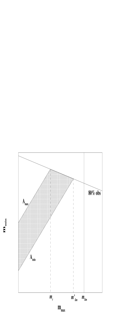
Figure 1: Principle of the selection function of the Hipparcos Input Catalogue (see text). The selected stars are located within the grey area.

3.2 Astrometric data

For every star of the sample, the coordinates, the parallax and the proper motion were found in the Hipparcos Catalogue (ESA esa97 (1997)). The parallax is negative for 48 Miras, 6 SRa and 8 SRb, but the LM algorithm is, by design, able to handle and exploit it.

For 309 stars, radial velocities were found in the Hipparcos Input Catalogue [HIC] (Turon et al. turon92 (1992)). Only 23 Miras, 3 SRa and 22 SRb have no RV data.

3.3 Magnitudes

The photometric data that we have chosen are $V$ (represented by visual measurements in this study), $J$ and $K$ magnitudes. $K$ was chosen because, for LPVs, its behaviour mimics relatively well the one of the bolometric magnitude. The $V-K$ colour is much more sensitive to the effective temperature and metallicity than $J-K$. On the other hand, the latter colour index is less affected by the presence of circumstellar dust shells, and it has the advantage that PLC relations using it have already been determined for the LMC.

Simple simulations have shown that, for LPV lightcurves with realistic amplitudes, periods and asymmetries, the mean magnitude differs from the mid–point value (average of the magnitudes at maximum and minimum brightness) by at most a few $10^{-1}$ in $V$ and a few $10^{-2}$ in $K$. We will thus use indifferently any of these two definitions in this study — actually the mid–point value for $V$ and the mean for $K$. Concerning the latter, it is worth noting that it also lies within less than 0.1 of the magnitude corresponding to the mean $K$ flux.

For most Miras and for 10 Semiregulars, the adopted visual magnitudes at maximum and minimum light are mean values calculated by Boughaleb (boughaleb95 (1995)) from AAVSO data covering 75 years (see Mennessier et al. mom97 (1997)). For 5 Miras, mean values of the max and min were deduced from AAVSO observations made during the whole Hipparcos mission. For 5 SR’s, we used means at max and min derived from the last 3 decades of AAVSO data.

For 26 Semiregulars, we adopted the mean $V$ magnitudes computed over decades by Kiss et al. (kiss99 (1999)), using the Fourier transform.

For the remaining 28 Miras and for most of the Semiregulars, the visual magnitudes at max and min are the ones given by the HIC.

We remind that the magnitudes at maximum and minimum brightness given by the Hipparcos Input Catalogue are either averages over decades, found in Campbell (campbell55 (1955)), or else estimated means derived from the GCVS (Kholopov et al. gcvs85 (1985), 1987). In the latter case, a statistical correction was applied to the catalogue values (and 1.5 mag subtracted in case of photographic magnitudes), as explained in the introduction of the HIC. For 4 Miras and 2 SRa’s for which the HIC magnitudes were adopted, we were able to check their consistency (within 0.1 mag) with the 25–year means published by the AAVSO (aavso86 (1986)).

The error bars of visual observations range from $\sigma=0.1$ to 0.5 mag according to the brightness. After binning and averaging, the precision at maxima is thus better than 0.1 mag; at minima, it may be worse. The derived mean magnitude is thus precise within about 0.2 mag. However, the uncertainty is larger for the mean maxima and minima derived from the GCVS extreme values: $\sigma=0.3$–0.4 mag according to our checking. Last, the error bars of the mean magnitudes derived by Kiss et al. (kiss99 (1999)) are, of course, negligible compared to the former ones. We may thus state that the overall precision of the mean visual magnitudes used in this study is about 0.2 mag for Miras and 0.2–0.4 mag for Semiregulars.

$J$ and $K$ magnitudes (with individual error bars of few $10^{-2}$ mag) were found in the Catalogue of Infrared Observations (Gezari et al. gezari96 (1996)) — which includes the large set of JHKL measurements of LPVs by Catchpole et al. (catchpo79 (1979)) and the measurements by Fouqué et al. (fouque92 (1992)) — and in recent papers: Groenewegen et al. (groene93 (1993)), Guglielmo et al. (gugliel93 (1993)), Whitelock et al. (whitelo94 (1994)), Kerschbaum & Hron (kersch94 (1994)) and Kerschbaum (kersch95 (1995)). The number of available data points per star ranges from 1 to more than 10, with an average of 1.5 for Miras and 2.2 for Semiregulars. As a consequence, considering the overall amplitude, which is usually $\la 1$ mag but may reach 1.5 mag for Miras, the error bars ($\sigma$) of the mean magnitude are a few $10^{-1}$ mag.

The mean colour indices $V-K$ and $J-K$ used in this study are the differences of the above defined mean magnitudes. The error bars are thus roughly 0.5 for the former and, since $J$ and $K$ measurements are usually made at the same phase, 0.05 mag for the latter.

Figure 2: Mean $V-K$ colour versus period of the sample stars (raw data).

3.4 Periods

For 26 Semiregulars, mean periods computed over decades were taken from Kiss et al. (kiss99 (1999)). For 21 other SR’s, the periods were computed over tens of cycles by Bedding & Zijlstra (bedding98 (1998)), Mattei et al. (mattei97 (1997)), Percy et al. (percy96 (1996)) and Cristian et al. (cristian95 (1995)).

For Miras and for the other Semiregulars, the adopted periods are the ones given by the HIC. Everytime possible (i.e. for nearly all Miras and for 10 SR’s), we have checked that they are very close to the 75–year means calculated by Boughaleb (boughaleb95 (1995)) from AAVSO data covering 75 years; the differences of a very few % correspond to the cycle–to–cycle fluctuations (see Mennessier et al. mom97 (1997)). For 4 Miras and 2 SRa’s, we were able to check that the HIC periods lie within 1–2 % of the 25–year means published by the AAVSO (aavso86 (1986)). Concerning the other stars, we can only guess the overall quality of the HIC by checking all stars used by Kiss et al. (kiss99 (1999)), Bedding & Zijlstra (bedding98 (1998)), Mattei et al. (mattei97 (1997)), Percy et al. (percy96 (1996)) and Cristian et al. (cristian95 (1995)): for SRa stars, only 4 % are found spurious (error $\ga 10\,\%$) and 83 % are very good (error $\la 3\,\%$); for SRb stars, about 25 % of the HIC periods appear spurious and 66 % very good.

As a consequence, about 15 % of the periods may be spurious in the sample of Semiregulars used in this paper.

3.5 Constraints

In addition to these individual data, it is known that O–rich LPVs in the LMC follow linear mean relations between the absolute magnitude ($M_{K}$ or $M_{\rm bol}$) and the logarithm of the period, and also near–infrared colour indices such as $(J-K)_{0}$ (Feast et al. feast89 (1989), Hughes & Wood hughes90 (1990), Hughes hughes93 (1993), Wood & Sebo wood96 (1996), Kanbur et al. kanbur97 (1997), Bedding & Zijlstra bedding98 (1998)). The existence of a linear {$M_{I}$, $\log P$} relation has also been shown (Feast et al. feast89 (1989), Pierce & Crabtree pierce93 (1993)). Moreover, Alvarez et al. (alvarez97 (1997)), applying to Hipparcos data an early version of the LM method that does not assume the existence of any PL or PLC relation, have shown that Oxygen–rich Miras in the solar neighbourhood do follow linear {$\log P$, $M_{K}$} relations. On the other hand, consistent with Kerschbaum & Hron (kersch92 (1992)), a simple plot of our raw data (see Fig. 2) strongly suggests that Miras and Semiregulars are distributed around at least two linear {$V-K$, $\log P$} relations, the one of Miras being peculiarly well–defined.

As a consequence, the calibrations presented in this series of papers have been performed under the assumption (constraint) that there exist in the sample such PLC relations whose de-biased coefficients are to be calculated by the algorithm. The validity of this choice is confirmed by the consistency of the so–derived luminosities with the ones found without making this assumption (Mennessier et al. mom99 (1999)).

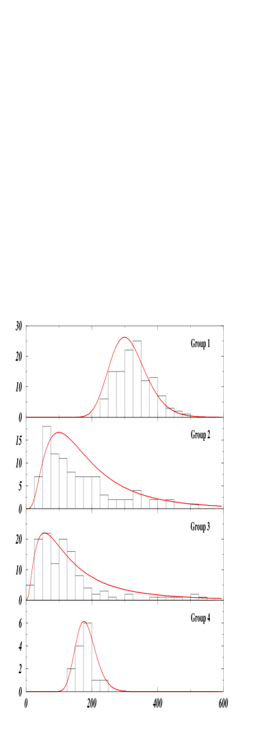
Figure 3: De-biased model period distributions (lines) and histograms of the data

Table 1: Model parameters of the four groups ($\theta$ denotes the fitted values and $\sigma$ their uncertainties)

	Group 1		Group 2		Group 3		Group 4
	$\theta$	$\sigma$	$\theta$	$\sigma$	$\theta$	$\sigma$	$\theta$	$\sigma$
$U_{0}$ [km/s]	-11.4	3.8	-33.8	5.9	-3.9	5.4	-33.1	66.2
$\sigma_{U}$	43.3	5.2	48.1	4.9	34.6	3.5	145.3	36.3
$V_{0}$ [km/s]	-31.9	5.0	-46.4	4.4	-19.1	1.8	-178.6	37.2
$\sigma_{V}$	29.8	2.0	37.9	4.5	17.5	3.3	102.4	26.3
$W_{0}$ [km/s]	-11.5	3.6	-10.8	5.1	-9.3	2.0	-4.8	30.6
$\sigma_{W}$	27.0	2.5	38.9	4.5	14.1	1.8	70.0	15.4
$Z_{0}$ [pc]	368	55	476	54	174	28
$\overline{\log P}$	2.48	0.01	2.00	0.06	1.75	0.06	2.24	0.03
$\sigma_{\log P}$	0.04	0.01	0.27	0.03	0.29	0.02	0.06	0.01
$\overline{(V-K)_{0}}$	8.47	0.11	5.75	0.13	6.19	0.28	5.56	0.46
$\sigma_{(V-K)_{0}}$	0.52	0.04	1.04	0.09	1.14	0.08	0.86	0.17
Cor.$(\log P,(V-K)_{0})$	-0.85	0.04	-0.46	0.07	-0.65	0.06	-0.49	0.44
${\mathfrak{m}}_{\mathfrak{c}}$	-4.0	2.4	-2.7	1.6	-4.0	1.3	1.8	1.5
%	31.8	0.02	29.3	0.03	34.9	0.03	3.9	0.02

4 Calibration and classification

The assumed number of model populations (groups) is constrained by the limited number of sample stars (357) and by the number of parameters to be fitted (18 per group). Its relevant value may be determined by means of a Wilks test (Soubiran et al. soubiran90 (1990), Wilks wilks63 (1963)). This test basically checks the significance of the likelihood increase obtained when the number of free parameters (in particular the number of groups) is increased. Considering that we are dealing with 2 or 3 types of variable stars and 2 or 3 galactic populations (Luri et al. 1996b , Alvarez et al. alvarez97 (1997)), several computations were carried out with 2, 3 and 4 groups. Wilks test indicated that the four–groups solution was still significant. Computation with five groups was not pursued until convergence because the number of free parameters was obviously too high (89 for 357 stars). To this respect, it is worth remarking that Group 1 was always clearly separated, while the other groups were mixed when less than 4 groups were used.

The fitted parameters of the model distributions corresponding to the 4–groups solution are given in Table 1 and in Sect. 5.1, with $1\sigma$ error bars derived from Monte Carlo simulations.

The de-biased model distributions of period are shown in Fig. 3.

The tridimensional {$P$, $M_{K}$, $(V-K)_{0}$} distributions of the calibrated data and of the model populations are displayed in Fig. 4.

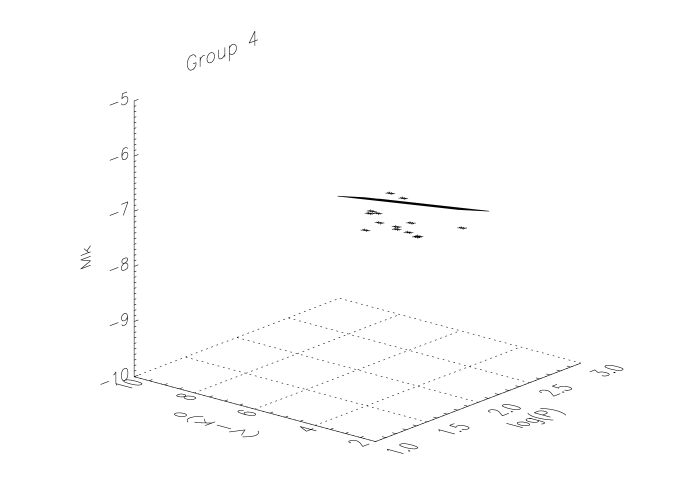
Figure 4: Calibrated period–luminosity–colour distributions: individual data and main symmetry plane (i.e. de-biased PLC relation) of the model distribution of each group.

The groups may get the following interpretation in terms of kinematics:

Group 1 (121 stars: 102 Miras, 6 SRa, 13 SRb) and Group 2 (96 stars: 54 SRb, 26 Miras, 16 SRa) have very similar kinematics, corresponding to old disk stars. Group 3 (125 stars: 102 SRb, 12 Miras, 11 SRa) has a younger kinematics than the previous ones. Group 4 (14 stars: 13 Miras, 1 SRa) has the kinematics of extended–disk or halo stars.

One can immediately see that the SRb stars constitute two populations of different ages. SRa stars are spread over all groups, with no clear “preference”. Most Miras appear in Group 1, with the same kinematics as the old SRb population.

5 Period—Luminosity—Colour relationship

5.1 PLC relations

The fitted distributions of period, magnitude and colour correspond to the following PLC relations (where the error bars correspond to $\pm 1\sigma$ deviations, as estimated using Monte Carlo simulations):

• Group 1:

  $$M_{K} =-1.07_{[\pm 0.50]}\log P -0.37_{[\pm 0.13]}(V-K)_{0}$$

  $$-1.49_{[\pm 0.72]}$$

  $\sigma_{M}\,=\,0.63_{[\pm 0.13]}$
  

• Group 2:

  $$M_{K} =-0.37_{[\pm 0.94]}\log P -0.42_{[\pm 0.24]}(V-K)_{0}$$

  $$-3.23_{[\pm 1.35]}$$

  $\sigma_{M}\,=\,0.32_{[\pm 0.17]}$
  

• Group 3:

  $$M_{K} =-1.69_{[\pm 0.54]}\log P -0.16_{[\pm 0.14]}(V-K)_{0}$$

  $$-2.53_{[\pm 0.78]}$$

  $\sigma_{M}\,=\,0.50_{[\pm 0.08]}$
  

• Group 4:

  $$M_{K} =-0.81_{[\pm 1.72]}\log P -0.09_{[\pm 0.45]}(V-K)_{0}$$

  $$-4.76_{[\pm 2.48]}$$

  $\sigma_{M}\,=\,0.48_{[\pm 0.21]}$
  

The coefficients of the relation found for Group 4 are obviously very uncertain. This is not surprising, in view of the small number of stars (15), their small dispersion, and the number of parameters to estimate. For Groups 1, 2 and 4, the error bars on the zero point are relatively large; this is due to the fact that the means of the three variables are far from zero, and thus any slope uncertainty rebounds magnified on the zero point.

5.2 Projection onto the {$P,M_{K}$} plane

The tridimensional model distributions may be projected onto the period–luminosity plane. The elliptic–looking lines shown in Fig. 5 are the projections of the isoprobability contours that, in the mean PLC plane, correspond to a $2\sigma$ deviation. The offset between the data and the model populations is due to the sampling bias, which is suppressed by the LM algorithm (see Appendix A for details). Then, Period–luminosity relations, liable to be compared to the ones observed in the Magellanic Clouds, are derived by means of a linear least–squares fit to the contours. Monte–Carlo simulations, as well as analytic computations, have shown that this is equivalent to a fit onto the projected population itself. Finally, the error bars of the coefficients are estimated, for each group, by applying the standard least–squares procedure to a simulated unbiased sample (thus they may be directly compared to the error bars usually given for the LMC stars).

The results are the following:

• Group 1:

  $$M_{K}=-5.04_{[\pm 0.72]}(\log P-2.48)-7.26_{[\pm 0.06]}$$

• Group 2:

  $$M_{K}=-1.13_{[\pm 0.16]}(\log P-2.00)-6.41_{[\pm 0.05]}$$

• Group 3:

  $$M_{K}=-2.11_{[\pm 0.13]}(\log P-1.75)-6.51_{[\pm 0.05]}$$

• Group 4:

  $$M_{K}=-1.37_{[\pm 2.32]}(\log P-2.24)-7.05_{[\pm 0.14]}$$

It may be noticed that Groups 2 and 3 have similar mean magnitudes. The same holds for Groups 1 and 4.

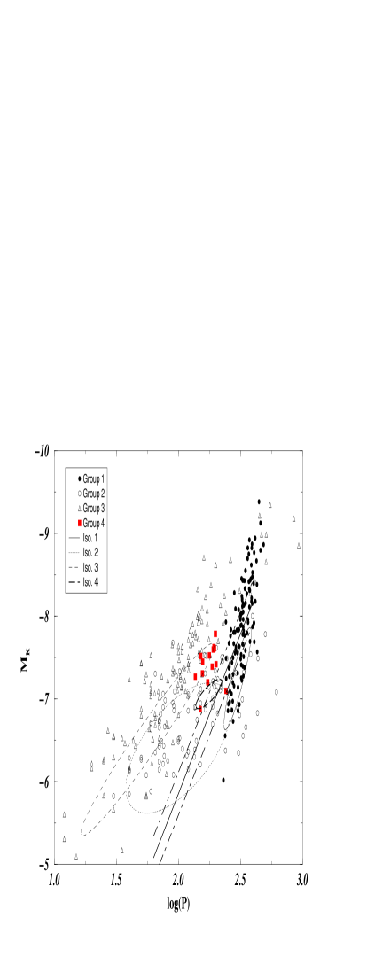
Figure 5: PL calibrated distributions: individual data and projected model distributions ($2\sigma$ isoprobability contours in the mean PLC plane). The Mira strip of the LMC is also shown (thick lines).

From a sample of 29 O–rich Miras of the Large Magellanic Cloud with period $\leq 420$ days, Feast et al. (feast89 (1989)) derived the following relation (were the error bars correspond to $1\sigma$ deviations):

$$M_{K}=-3.47_{[\pm 0.19]}\log P+0.93_{[\pm 0.45]}$$

$$\sigma_{M}=0.13$$

assuming a distance modulus of 18.55.

Based on a sample of more than a hundred Oxygen–rich Miras of the LMC, the solution of Hughes & Wood (hughes90 (1990)) is, under the same assumptions:

$$M_{K}=-3.86_{[\pm 0.18]}(\log P-2.4)-7.40_{[\pm 0.02]}$$

$$\sigma_{M}=0.26$$

From a sample of 79 Miras, unfortunately including a significant number of Carbon stars, Hughes (hughes93 (1993)) derived:

$$M_{K}=-3.75_{[\pm 0.14]}(\log P-2.4)-7.45_{[\pm 0.02]}$$

$$\sigma_{M}=0.13$$

Obviously, the slopes are significantly different from that of any Galactic PL relation found above. Such a difference was also observed between the LMC and Globular Clusters stars by Menzies & Whitelock (menzies85 (1985)). It cannot be due to the well–known steepening of the PL relation at periods larger than 420 days, i.e. relatively high mass (Feast et al. feast89 (1989)), since only a very few sample stars may be concerned. The first possible explanation is that the so–called Miras of the LMC include, in fact, a significant number of SRb semiregulars, especially at “short” periods. Indeed, for the outer galaxies, the observers use to call “Miras” the LPVs with an amplitude larger than a given threshold (e.g. 0.9 mag in $I$), corresponding to the maximum amplitude of SRa stars according to the GCVS. This criterium is obviously not sufficient and the slope of the so–called LMC “Mira” strip should then be intermediary between our Groups 1 and 2. A second explanation of the slope discrepancy is that the shorter–period “Miras” in the LMC include a population more–or–less equivalent to our Group 4, i.e. metal–deficient with a mean mass similar to or lower than the one of the main population. This, too, would lead to a shallower global PL relation. The existence of such a population had been suggested by Wood et al. (wood85 (1985)) and Hughes et al. (hughes91 (1991)). Of course, these two explanations do not exclude each other.

It is also worth noting that the PL slopes of Groups 2 and 3 are much smaller than the one of Group 1 (Miras), and similar to the one of the evolutionary tracks ($-1.67$), derived by Bedding & Zijlstra (bedding98 (1998)) from the works of Whitelock (whitelo86 (1986)) and Vassiliadis & Wood (vassili93 (1993)). Moreover, in Group 2 as well as in Group 3, the proportion of SRb’s (as defined by the GCVS) decreases towards longer periods: at $P>200$ days, they represent less than 25 % of the stars of these groups, while Miras (GCVS) amount to 45 % for Group 2 and 65 % for Group 3. All of this indicates that, in each population, the sequence of SRb Semiregulars corresponds to an evolutionary sequence towards the Mira instability strip.

5.3 Projection onto the {$P$, $V-K$} plane

In the same way as in the preceding subsection, a linear fit to the projected model distributions (see Fig. 6) yields the following period–colour relations:

• Group 1:

  $$(V-K)_{0}=10.80_{[\pm 0.58]}(\log P-2.48)+8.51_{[\pm 0.05]}$$

• Group 2:

  $$(V-K)_{0}=1.80_{[\pm 0.32]}(\log P-2.00)+5.75_{[\pm 0.10]}$$

• Group 3:

  $$(V-K)_{0}=2.54_{[\pm 0.28]}(\log P-1.75)+6.20_{[\pm 0.10]}$$

• Group 4:

  $$(V-K)_{0}=6.50_{[\pm 2.47]}(\log P-2.24)+5.52_{[\pm 0.15]}$$

The difference of slope between Groups 2 and 3 is (qualitatively) consistent with the differences of mass and metallicity expected from the kinematics. Indeed, the larger mass of Group 3 stars yields significantly higher temperatures and thus a larger {$T_{\rm eff},(V-K)$} slope, while the moderate metallicity difference has only a small influence (Bessell et al. bessell89 (1989, 1998)). This is due to the behaviour of the TiO lines in this temperature range.

On the other hand, the much larger slope of Group 1 may be explained by a difference of pulsation mode, consistently with the larger mean period. Indeed, the period of a lower–order mode must be more sensitive to the temperature (see, e.g., Barthès barthes98 (1998)).

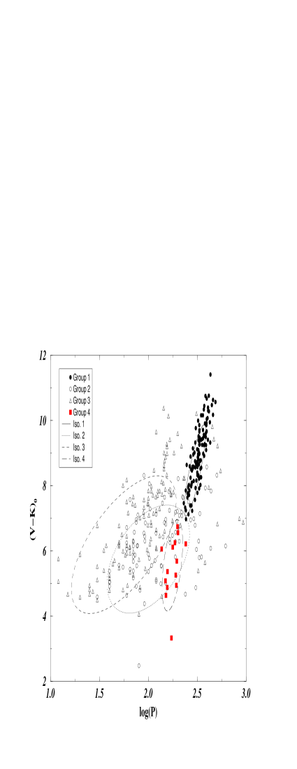
Figure 6: PC calibrated distributions: individual data and projected model distributions.

5.4 Projection onto the {$M_{K}$, $V-K$} plane

The calibration results in the Luminosity–Colour plane are shown in Fig. 7. As explained in the Appendix A, the offset and the difference of width between the data distributions and the projected $2\sigma$ contours are effects of the projection and of the sampling bias. A linear fit to the contours yields the following luminosity–colour relations:

• Group 1:

  $$M_{K}=-0.42_{[\pm 0.05]}((V-K)_{0}-8.47)-7.24_{[\pm 0.05]}$$

• Group 2:

  $$M_{K}=-0.45_{[\pm 0.03]}((V-K)_{0}-5.75)-6.41_{[\pm 0.03]}$$

• Group 3:

  $$M_{K}=-0.34_{[\pm 0.04]}((V-K)_{0}-6.19)-6.51_{[\pm 0.06]}$$

• Group 4:

  $$M_{K}=-0.10_{[\pm 0.17]}((V-K)_{0}-5.56)-7.06_{[\pm 0.14]}$$

As in the preceding subsection, the difference of slope between Groups 2 and 3 is easily explained by the temperature–dependence of the {$T_{\rm eff},(V-K)$} slope, which is little sensitive to moderate metallicity variations.

Figure 7: LC calibrated distributions: individual data and projected model distributions.

5.5 {P, $J-K$} distribution

Once the distances have been calibrated, it is possible to check the distribution of the sample stars with respect to the de-reddened $J-K$ index. The results are shown in Fig. 8, together with the raw data.

The $J-K$ Period–Colour distribution appears similar to the $V-K$ one. The scattering, also existing in the raw data, makes the PC relation more difficult to see. It is due to the smaller number of stars in the $J$ data set, and probably also to the peculiar sensitivity of this colour index to the surface gravity and extension of the envelope (Bessell et al. bessell89 (1989, 1998)).

A linear least–squares fit to the de-reddened data (excluding a few obviously misclassified stars, namely two having $(J-K)_{0}>2$ and two having $(J-K)_{0}<0.6$) yields:

• Group 1 (86 stars):

  $$(J-K)_{0}=1.01_{[\pm 0.22]}\log P-1.27_{[\pm 0.56]}$$

  $$\sigma_{J-K}=0.02$$

• Group 2 (63 stars):

  $$(J-K)_{0}=0.16_{[\pm 0.07]}\log P+0.83_{[\pm 0.14]}$$

  $$\sigma_{J-K}=0.02$$

• Group 3 (91 stars):

  $$(J-K)_{0}=0.17_{[\pm 0.04]}\log P+0.85_{[\pm 0.08]}$$

  $$\sigma_{J-K}=0.02$$

• Group 4 (12 stars):

  $$(J-K)_{0}=1.02_{[\pm 0.67]}\log P-1.25_{[\pm 1.51]}$$

  $$\sigma_{J-K}=0.01$$

These fit relations are probably slightly biased, and thus should be shifted by a certain amount so as to represent the whole populations.

Contrary to what was found with $V-K$, the relations of Groups 2 and 3 cannot be reliably distinguished here. This may be due to the crossing–over of the iso–metallicity curves in the {$T_{\rm eff},J-K$} diagram: the effects of the differences of temperature and metallicity between the two groups tend to compensate each–other (Bessell et al. bessell89 (1989, 1998)).

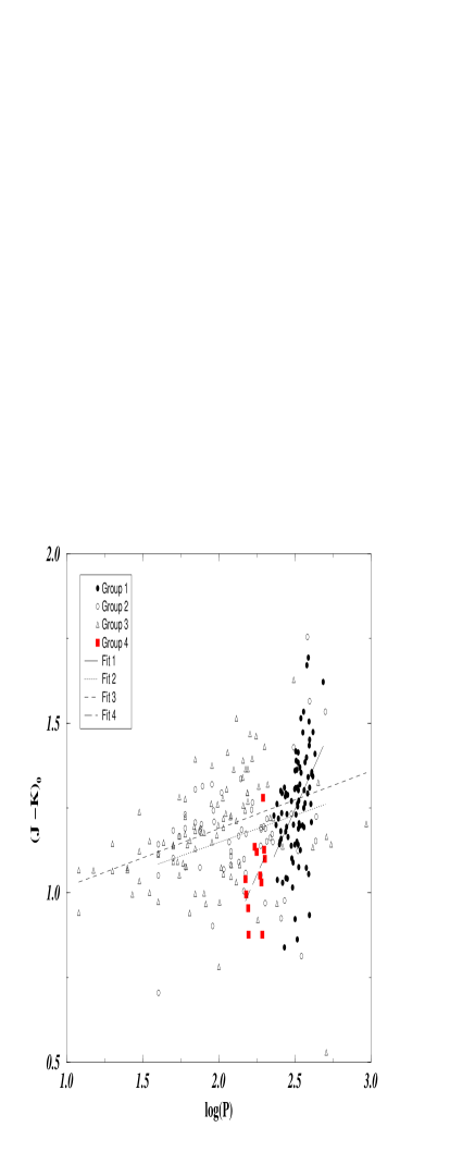
Figure 8: $J-K$ versus Period distribution of sample stars: raw (top) and dereddened (bottom) indices. Two stars with $J-K>2$ are not shown.

Based on 29 Oxygen Miras, the relation found by Feast et al. (feast89 (1989)) for the LMC is:

$$(J-K)_{0}=0.56_{[\pm 0.12]}\log P-0.12_{[\pm 0.29]}$$

$$\sigma_{J-K}=0.08$$

From a sample of 21 stars, Hughes (hughes93 (1993)) derived:

$$(J-K)_{0}=0.37_{[\pm 0.05]}(\log P-2.4)+1.215_{[\pm 0.014]}$$

$$\sigma_{J-K}=0.06$$

As for the PL relation, we find a significant discrepancy between the Miras in the LMC and the ones in the solar neighbourhood. Since, in $J-K$ as well as in $V-K$, Group 4 is approximately aligned with Group 1, and thus metal–deficient Miras of the LMC should not significantly influence its PC relation, it seems that, as suggested in Sect. 5.2, we are actually encountering a problem of misclassification of the LPVs in the outer galaxies. This, of course, does not preclude the existence of a metal–deficient population which would further influence the PL relation.

5.6 {$M_{K}$, $J-K$} distribution

The LC relations yielded by a linear least–squares fit to the calibrated and de-reddened data are:

• Group 1:

  $$M_{K}=-1.22_{[\pm 0.39]}(J-K)_{0}-6.32_{[\pm 0.49]}$$

  $$\sigma_{M}=0.33$$

• Group 2:

  $$M_{K}=-1.37_{[\pm 0.37]}(J-K)_{0}-5.24_{[\pm 0.44]}$$

  $$\sigma_{M}=0.22$$

• Group 3:

  $$M_{K}=-2.39_{[\pm 0.59]}(J-K)_{0}-4.41_{[\pm 0.70]}$$

  $$\sigma_{M}=0.69$$

• Group 4:

  $$M_{K}=-0.18_{[\pm 0.65]}(J-K)_{0}-7.25_{[\pm 0.68]}$$

  $$\sigma_{M}=0.06$$

We remind that these fit relations are subject to sampling bias, and thus should be significantly shifted downwards, so as to represent the whole population (see Appendix A).

In view of the error bars, the slope of Group 3 may be the same as the one of Groups 1 and 2, which is what is expected from AGB evolutionary models. This supports our interpretation of the slope differences found in $V-K$ (Sect. 5.4). The slope of Group 4 is, once again, not reliable.

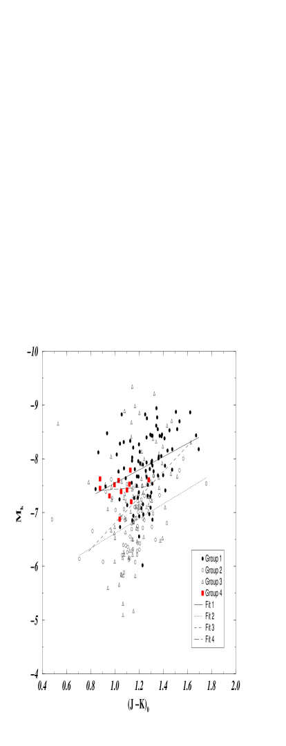
Figure 9: Magnitude versus $(J-K)_{0}$ distribution of the sample stars, deduced from the luminosity calibration.

6 Conclusions

Thanks to an up–to–date maximum–likelihood method, using parallaxes, proper motions, radial velocities and other independent data (periods and colours), we have calibrated the luminosity of about 350 Oxygen–rich Long–Period Variable stars (Miras, SRa and SRb) observed by Hipparcos. Meanwhile, the stars got classified in several groups differing by their distributions of kinematical parameters, magnitude, period and colour. Four groups were found: Group 1, mainly composed of Miras and having the kinematics of old disk stars; Group 2, mainly composed of SRb, with the same kinematics as Group 1; Group 3, also mainly composed of SRb, but with a much younger kinematics; Group 4, corresponding to the extended disk and halo, and containing no SRb. For each of them, we obtained de–biased PLC, PL, PC and LC relations.

We thus confirm the existence of two SRb populations, already suggested on other grounds by Kerschbaum & Hron (kersch92 (1992, 1994)).

SRa stars do not seem to constitute a separate class. They can be considered as a small–amplitude subset of the Mira and SRb classes.

The presence of a small but significant number of Miras in Group 2, and of SRb’s in Group 1, may be due to the probabilistic character of our classification method. However, it also tends to confirm that the usual (GCVS) classification criteria are not fully pertinent, as shown by Lebzelter et al. (lebz95 (1995)).

As expected, since they all belong to the AGB, the stars seem to obey a global luminosity–colour relation, both in $(V-K)_{0}$ and $(J-K)_{0}$. More precisely, each group has its own relation, nearly parallel to the others, with a slight shift.

Though belonging to the same Galactic population, Group 2 stars (SRb’s) are fainter, bluer, and have shorter period and shallower period–colour relation than Group 1 (Miras). They probably pulsate on a higher–order mode. The higher luminosity and shorter period of Group 3 with respect to Group 2 is probably due to higher mass and metallicity. The slope of Groups 2 and 3 in a period–luminosity diagram, as well as a close look at the distribution of the three variability types within these groups, indicate that the two sequences of Semiregulars correspond to evolutionary sequences towards the Mira instability strip (i.e. SRb’s are, generally, a little younger than Miras of the same population).

All these findings will be confronted in detail to theoretical models of pulsation and evolution in Paper II.

Another important result of our study is that, contrary to a usual assumption (e.g. in van Leeuwen et al. [vanleeuw97 (1997)]), but consistently with the work of Menzies & Whitelock (menzies85 (1985)) on a few Globular Cluster stars, the PL and PC relations of Oxygen–rich Miras found in the LMC may not be trivially transposed to other galaxies by simply shifting the zero–point: their slopes are inconsistent with the ones found for O–rich Miras in the solar neighbourhood.

The first explanation is a misclassification of many LMC stars, since the observers simply discriminated the SRa stars on grounds of their small amplitude, and thus the remaining so–called “Miras” included a significant proportion of (younger) SRb stars. Concerning the PL relations, additional discrepancy may be generated by a metal–deficient, probably older LMC Mira population, the existence of which was already suspected by Wood et al. (wood85 (1985)) and Hughes et al. (hughes91 (1991)). All this, together with the fact that the stars distribution within the LMC “Mira” strip (at least below 500 days) seems rather uniform, suggests that these LPVs derive from a quite smooth star formation history, rather than well–separated bursts.

Concluding, the fact that the global PL relation of LMC “Miras” approximately matches the global one of Galactic Miras (in the solar neighbourhood) does not guarantee that it holds for every galaxy: everything depends on the relative number of misclassified SRb’s and on the respective proportion of the different populations of stars, i.e. on the star formation history.

Nevertheless, consistently with the LMC and globular clusters data (see e.g. Hughes & Wood hughes90 (1990) and Menzies & Whitelock menzies85 (1985)), our calibrations show that an LPV M–giant (Mira, SRa or SRb) pulsating with a period of 300–330 days is expected to have a mean absolute $K$ magnitude of $-7.5\pm 0.5$, whatever the stellar population. This may be used as a distance estimator.

Appendix A Populations, sampling and biases

A striking feature of Figs. 5 through 7 is that many stars are located outside, most often above the projected $2\sigma$ contour of the fitted distribution of the corresponding group, whereas one would expect most of them to be located inside or symmetrically around it.

First, one must remember that, in the PL and LC diagrams, the projected $2\sigma$ contour (i.e. the projection of the $2\sigma$ contour of the mean PLC plane) is not the $2\sigma$ contour of the projected distribution. This explains why, in the Luminosity–Colour diagram (Fig. 7), the width of each sequence of sample stars is much larger than the corresponding “ellipse”.

On the other hand, the offset of the sample distributions with respect to the model ones is due to the fact that the sample selection is based on the apparent magnitude (see Sec. 3.1). This is analogous to the Malmquist bias. To better understand the phenomenon in our case, a closer look at this well known bias may be helpful:

Malmquist (malm36 (1936)) studied the bias in the mean absolute magnitude that is derived from a sample of stars with the following characteristics:

• The base population from which the sample is extracted has (a) a homogeneous spatial distribution and (b) a Gaussian distribution of absolute magnitudes $G(M_{0},\sigma_{M})$

• The sample is selected within the base population by means of a limit–magnitude criterium: $m\leq m_{lim}$

Under these conditions, Malmquist (malm36 (1936)) proved that the mean absolute magnitude of the sample $<M>$ differs from the mean absolute magnitude of the base population $M_{0}$ according to: $<M>=M_{0}-1.38\;\sigma_{M}^{2}$ .

In other words, the stars in the sample are, on average, brighter that the base population. The reason for this is that, because of the apparent magnitude limit, brighter stars are over–represented in the sample: as they can be seen at longer distances, more of them are included.

In our case, the effects are more complicated (inhomogeneous spatial distribution, PLC relations and complex selection function) and also stronger. The PLC relations have, in some cases, large slopes and thus the groups may contain stars of very different absolute magnitudes. Like in the case of the Malmquist bias, brighter stars are favoured and thus over–represented in our sample. This favours, in turn, stars with long periods and large colour indices but also, at a given period and colour, stars located on the “bright” side of the main PLC plane.

Figure 10: Simulated sample of Group 1 stars with no magnitude limit.

Figure 11: Same simulation when applying the magnitude–based selection function.

This effect can be illustrated by Monte-Carlo simulations. Let us first simulate a sample of Group 1 stars with no magnitude limit. As can be seen in Fig. A1, most of these stars are located, in the $\{\log P,M_{K}\}$ plane, inside the projected $2\sigma$ contour of the distribution used for the simulation. However, when the selection function (the one whose parameters were calculated in Sect. 4) is applied, the $\{\log P,M_{K}\}$ distribution of the sample drastically changes, as shown in Fig. A2: in this case, a majority of the stars are brighter than the projected $2\sigma$ contour.

This example clearly shows that the suprising peculiarities of Figs. 5 to 7 are nothing but natural. Moreover it shows that, in the most general case, a “naive” fit to the absolute magnitude distribution of a sample is not at all representative of the base population. Fortunately, this bias is probably negligible in the case of Magellanic Clouds studies, since all their LPVs may be considered as located at the same distance with a reasonable approximation, and their amplitudes are small in the near–infrared bands where they are observed.

References

- (1) AAVSO, 1986, Maxima and minima of Long–Period Variables, 1949–1975, AAVSO Pub.
- (2) Alvarez R., Mennessier M.O., Barthès D., Luri X., Mattei J.A., 1997, A&A 327, 656
- (3) Arenou F. , Grenon M. , Gómez A.E., 1992, A&A 258, 104
- (4) Barthès D., 1998, A&A 333, 647
- (5) Barthès D., Luri X., 1999, A&A, (paper II) in preparation
- (6) Barthès D., Luri X., Alvarez R., Mennessier M.O., 1999, A&A, (paper III) in preparation
- (7) Bedding T.R., Zijlstra A.A., 1998, ApJ 506, L47
- (8) Bessell M.S., Brett J.M., Scholz M., Wood P.R., 1989, A&AS 77, 1
- (9) Bessell M.S., Castelli F., Plez B., 1998, A&A 333, 231
- (10) Boughaleb H., 1995, PhD thesis, Université Montpellier II
- (11) Brown A.G.A., Arenou F., Van Leeuwen F., Lindegren L., Luri X., 1997, In: Hipparcos Venice’97, ESA SP-402, p. 63
- (12) Campbell L., 1955, Studies of Long–Period Variables, AAVSO Pub.
- (13) Catchpole R.M., Robertson B.S.C., Lloyd Evans T.H.H., Feast M.W., Glass I.S., Carter B.S., 1979, SAAO Circ. 1, 61
- (14) Cristian V.C., Donahue R.A., Soon W.H., Baliunas S.L., Henry G.W., 1995, PASP 107, 411
- (15) ESA, 1997, The Hipparcos and TYCHO Catalogue, ESA SP-1200
- (16) Feast M.W., Glass I.S., Whitelock P.A., Catchpole R.M., 1989, MNRAS 241, 375
- (17) Fouqué P., Le Bertre T., Epchtein N., Guglielmo F., Kerschbaum F., 1992, A&AS 93, 151
- (18) Gezari D.Y., Pitts P.S., Schmitz M., Mead J.M., 1996, Catalog of Infrared Observations (edition 3.5), available from VizieR
- (19) Groenewegen M.A.T., De Jong T., Baas F., 1993, A&AS 101, 513
- (20) Guglielmo F., Epchtein N., Le Bertre T., Fouqué P., Hron J., Kerschbaum F., Lepine J.R.D., 1993, A&AS 99, 31
- (21) Howell S.B., 1982, PASP 94, 969
- (22) Hughes S.M.G., 1993, In: Nemec J.M., Matthews J.M (eds.), New Perspectives on Stellar Pulsation and Pulsating Variable Stars, Cambridge Univ. Press, p. 192
- (23) Hughes S.M.G., Wood P.R., 1990, AJ 99, 784
- (24) Hughes S.M.G., Wood P.R., Reid N., 1991, AJ 101, 1304
- (25) Kanbur S.M., Hendry M.A., Clarke D., 1997, MNRAS 289, 428
- (26) Kerschbaum F., 1995, A&AS 113, 441
- (27) Kerschbaum F., Hron J., 1992, A&A 263, 97
- (28) Kerschbaum F., Hron J., 1994, A&AS 106, 397
- (29) Kholopov P.N., 1985, 1987, General Catalogue of Variable Stars, Nauka, Moscow
- (30) Kiss L.L., Szatmáry K., Cadmus R.R. Jr., Mattei J.A., 1999, A&A (preprint)
- (31) Lebzelter T., Kerschbaum F., Hron J., 1995, A&A 298, 159
- (32) Luri X., 1995, PhD Thesis, Universitat de Barcelona
- (33) Luri X., Mennessier M.O., Torra J., Figueras F., 1996a, A&AS 117, 405
- (34) Luri X., Mennessier M.O., Torra J., Figueras F., 1996b, A&A 314, 807
- (35) Malmquist K.G., 1936, Stockholms Ob. Medd. 26
- (36) Mattei J.A., Foster G., Hurwitz L.A., Malatesta K.H., Willson L.A., Mennessier M.O., 1997, In: Battrick B. (ed.), Hipparcos Venice ’97, ESA SP-402, p. 269
- (37) Mennessier M.O., Baglin A., 1988, In: Torra J. & Turon C. (eds.), Scientific aspects of the Hipparcos Input Catalogue Preparation II., CIRIT (Generalitat de Catalunya), p. 361
- (38) Mennessier M.O., Boughaleb H., Mattei J.A., 1997, A&AS 124, 1
- (39) Mennessier M.O., Alvarez R., Luri X., Noirhomme–Fraiture M., Rouard E., 1999, In: Le Bertre T., Lèbre A., Waelkens C. (eds.), Asymptotic Giant Branch Stars (Proc. IAU Symp. 191), PASP, p. 117
- (40) Menzies J.W., Whitelock P.A., 1985, MNRAS 212, 783
- (41) Percy J.R., Desjardins A., Yu L., Landis H.J., 1996, PASP 108, 139
- (42) Pierce M.J., Crabtree D.R., 1993, In: Nemec J.M., Matthews J.M (eds.), New Perspectives on Stellar Pulsation and Pulsating Variable Stars, Cambridge Univ. Press, p. 102
- (43) Soubiran C., Gómez A.E., Arenou F., Bougeard M.L., 1990, In: Jaschek & Murtagh (eds.), Errors, bias and uncertainties in astronomy, Cambridge Univ. Press, p. 408
- (44) Turon C., Crézé M., Egret D., et al., 1992, The Hipparcos Input Catalogue, ESA SP-1136
- (45) Van Leeuwen F., Feast M. W., Whitelock P.A., Yudin B., 1997, MNRAS 287, 955
- (46) Vassiliadis E., Wood P.R., 1993, ApJ 413, 641
- (47) Whitelock P., 1986, MNRAS 219, 525
- (48) Whitelock P., Menzies J., Feast M., Marang F., Carter B., Roberts G., Catchpole R., Chapman J., 1994, MNRAS 267, 711
- (49) Wilks S., 1963, Mathematical statistics, Wiley
- (50) Wood P.R., Bessell M.S., Paltoglou G., 1985, ApJ 290, 477
- (51) Wood P.R., Sebo K.M., 1996, MNRAS 282, 958