Calibration of the MACHO Photometry Database

Abstract

The MACHO Project is a microlensing survey that monitors the brightnesses of $\sim$60 million stars in the Large Magellanic Cloud (LMC), Small Magellanic Cloud, and Galactic bulge. Our database presently contains about 80 billion photometric measurements, a significant fraction of all astronomical photometry. We describe the calibration of MACHO two-color photometry and transformation to the standard Kron-Cousins $V$ and $R$ system. Calibrated MACHO photometry may be properly compared with all other observations on the Kron-Cousins standard system, enhancing the astrophysical value of these data. For $\sim$9 million stars in the LMC bar, independent photometric measurements of $\sim$20,000 stars with $V\lower 2.15277pt\hbox{$\,\buildrel<\over{\sim}\,$}18$ mag in field-overlap regions demonstrate an internal precision $\sigma_{V}=0.021$, $\sigma_{R}=0.019$, $\sigma_{V-R}=0.028$ mag. The accuracy of the zero-point in this calibration is estimated to be $\pm 0.035$ mag for stars with colors in the range $-0.1<(V-R)<1.2$ mag. A comparison of calibrated MACHO photometry with published photometric sequences and new Hubble Space Telescope observations shows agreement. The current calibration zero-point uncertainty for the remainder of the MACHO photometry database is estimated to be $\pm 0.10$ mag in $V$ or $R$ and $\pm 0.04$ mag in $(V-R)$. We describe the first application of calibrated MACHO photometry data: the construction of a color-magnitude diagram used to calculate our experimental sensitivity to detect microlensing in the LMC.

(The MACHO Collaboration)

1 Introduction

The MACHO Project is a microlensing survey experiment (Alcock et al. 1997) that monitors the brightness variations of $\sim$60 million stars in the Large Magellanic Cloud (LMC), Small Magellanic Cloud (SMC) and Galactic bulge. Microlensing is the rare transient magnification of a background source star due to the gravitational effect of a massive compact object crossing the line of sight. Paczyński (1986) first noted that if the dynamically-inferred Galactic dark halo was composed of massive compact objects, the probability of microlensing would be $\tau\sim 5\times 10^{-7}$ toward the LMC, within reach of dedicated observational surveys. The MACHO Project survey observations are made with a mosaic of charge-coupled devices imaging simultaneously in non-standard blue and red passbands. The special purpose instrument is permanently mounted on the 50-inch Great Melbourne Telescope in Australia (Hart et al. 1996). The total sky area monitored is approximately 40, 3, and 45 square degrees in the LMC, SMC, and Galactic bulge, respectively. Each star is represented in the MACHO database by a time-series of two-color photometric measurements. In some cases, stars are counted in the database two or three times because the survey fields overlap on the sky.

In this paper, we describe the calibration of MACHO photometry data. Calibration actually encompasses several levels of detail regarding the systematic transformation of the MACHO data to a meaningful absolute system. The first level of calibration is the creation of an instrumental system. The second level of calibration is the transformation of the instrumental photometry to the Kron-Cousins $V$ and $R$ standard system. This level of calibration allows for proper comparison of MACHO data with all other data on this system. In practice, these two levels of calibration are not implemented separately. The third level of calibration discussed in this paper is the calibration of lightcurves, i.e. analysis-stage corrections that may be applied to time-series photometric data for individual stars. These corrections will eliminate some systematic sources of scatter in the photometry. Our first effort is to calibrate the “top-22” LMC fields analysed in Alcock et al. (1997).

The MACHO Project microlensing analyses involve the photometric calibration in a number of ways. First, regions of the LMC color-magnitude diagram (CMD) excluded in the search for microlensing because of the high background of intrinsic variable stars are more accurately defined with the calibrated data. It is also possible to make a more precise comparison of the distribution of microlensing source stars in the CMD with that expected for true microlensing. Finally, calibration plays an important role in the analysis of LMC microlensing through the calculation of our experimental sensitivity to detect microlensing, which we will call the “efficiency.”

The microlensing efficiency calculation requires a critical assumption regarding the true distribution of stars in the LMC for the following reason. Individual stars in the ground-based MACHO image data are almost always confused, i.e. they are composites of two or more unresolved companions. However, only one true LMC star will be lensed. The partial magnification of flux from an unresolved, composite star is an effect known as blending in microlensing. Observational data and further discussion of blending can be found in Alcock et al. (1997). It is useful to distinguish an apparent star in the MACHO data which is actually a blend of several real “stars” by referring to it as an “object.” The efficiency calculation (an exhaustive series of artifical star tests and Monte-Carlo experiments) returns our experimental sensitivity to detect microlensing of stars, not objects.

In order to quantify the ratio of stars to objects, we have obtained Hubble Space Telescope (HST) imaging data in their filter equivalents of $V$ and $R$ for three fields in the LMC top-22. The high spatial resolution of the HST allows us to probe to fainter magnitudes than possible with our ground-based data, particularly in the crowded bar region. The HST and MACHO data are properly comparable after their respective calibration to the Kron-Cousins standard $V$ and $R$ magnitude system. We construct the “efficiency CMD”, which is a properly scaled splicing of MACHO and HST data together into a CMD that also contains accurate information on the numbers of stars. The scaling factor is essentially the sought-after star to object ratio. The efficiency CMD described here has been used to seed millions of artificial stars into our raw image data, and is the first application of calibrated MACHO data. Complete discussions of the new LMC microlensing analysis, the efficiency calculation, and the HST data reduction are beyond the scope of this paper; each will be the subject of a forthcoming paper.

In addition to microlensing, the MACHO photometry database is a valuable resource for studying the stellar populations and star formation history of the LMC, making new tests of stellar evolution theory, and for studying variable stars. Calibration enhances the value of the MACHO database for these so-called science “by-products.” For this reason, we give special attention to details of the calibrations that may be relevant to consumers of released MACHO data.

Our paper is organized as follows. In §2, we preface the calibration discussion with some details of the MACHO image and photometry data. In §3, we review the calibration of the LMC top-22 fields. In §4, we compare the calibrated MACHO data with a sample of published photometric sequences in the LMC and with the new HST observations. In §5, we describe the status of calibration for the remaining fields in the LMC, SMC, and Galactic bulge. In §6, we review the calibration of MACHO instrumental lightcurves. In §7, we examine the HST and MACHO data in greater detail and construct the efficiency CMD. Finally, §8 is the summary of our results.

2 MACHO Data

2.1 Images

The MACHO experiment has dedicated use of the 1.27-m (50-inch) Great Melbourne Telescope (Robinson & Grubb 1869), now located at the Mount Stromlo Observatory in Australia. A system of corrective optics has been installed at the prime focus, giving a focal reduction to $f/3.9$ and a $1^{\circ}$ field of view. A dichroic beam-splitter enables simultaneous blue and red imaging (Hart et al. 1996). Observations may be made from either side of the telescope pier (a German equatorial mount), i.e. either an East or West of pier observation. The median stellar image FWHM is 2 arcsec. The typical sky for an LMC bar field is estimated to be $R$ $\sim$ 19.5 mag per square arcsec.

The MACHO filters were specially designed to provide an adequate color index and wide bandpasses. The blue filter runs from $\sim$4500$-$6300 $\AA$ and the red filter runs from $\sim$6300$-$7600 $\AA$. At both the red and blue foci, a mosaic of four 2048$\times$2048 Loral charge coupled devices (CCDs) are mounted. In Figure 1, we show the approximate response of the dichroic, filters, and CCDs. The wide-field optics corrector has not been included. Uncertainty is estimated to be $\sim$20% in these response functions. The normalized standard $BVRI$ passbands from Bessell (1990) are also shown.

The Loral CCD pixel size is $15\,\mu m$ which corresponds to $0.^{\prime\prime}635$ on the sky, giving a sky coverage of $0.52$ square degrees per MACHO field. Each CCD has two read-out amplifiers, and the images are read-out through a 16-channel system and written into dual-ported memory in the data acquisition computer. The readout time is 67 seconds per image, and the noise is $\sim 10$ electrons rms, with a gain of $\sim 2\,e^{-}$/ADU. Further details of the MACHO camera system are provided in Stubbs et al. (1993) and Marshall (1994).

In Figure 2, we present a schematic drawing of the red and blue MACHO focal planes from both the East and West sides of the pier. We label each CCD (0-3 on the red side, and 4-7 on the blue side), and each amplifier (.0 or .1). The CCD-amplifier designated 0.0 is inoperative; it is marked with an “X.” For the purposes of photometry, each red and blue MACHO image is divided into 64 “chunks” (128 total), each approximately $512\times 512$ pixels in size. Chunks are defined as regions of a certain CCD and amplifier in the MACHO focal plane. Every red chunk uniquely corresponds to a blue chunk. In the bottom two panels of Figure 2, we present chunk maps in the West of pier orientation.

2.2 SoDOPHOT

The photometry for the MACHO experiment is handled by a special purpose code called SoDOPHOT, which stands for “Son of DOPHOT.” The reader is referred to Schecter, Mateo, and Saha (1993) for further details of DOPHOT. Briefly, it is a model-based fitting code that searches for objects in two dimensional digital array images of the sky. Stars, galaxies, cosmic rays, and so forth are each assigned a specific model defined in terms of analytic functions. Objects are identified and photometered with precise signal-to-noise criteria based on the model fits. DOPHOT may tend to report brighter magnitudes for faint stars in crowded regions than Daophot (Stetson 1987), a similar type of photometry code that is widely employed by astronomers. This systematic effect is attributed to the sky fitting procedure (Schecter et al. 1993), and is likely preserved in SoDOPHOT.

SoDOPHOT is basically DOPHOT optimized to the MACHO image data and modified for extremely fast CPU reduction times. Most of the improvement in speed can be attributed to the fact that we observe the same fields repeatedly. We designate a high quality image of a given field as a “template” image and use the reduction of our template image to help with the reduction of the other images. The template starlists are generated by an iterative and automated DOPHOT reduction which employs both the red and blue MACHO template images.

For routine reductions, SoDOPHOT makes a list of stellar positions and brightnesses of the brightest stars in the new image and finds a crude transformation to the positions and relative brightness of stars from the template. This transformation is then used to find the approximate location of a set of about 40 bright and relatively isolated fiducial stars per chunk which have been preselected from the list of template stars. SoDOPHOT reductions are done on individual chunks, i.e. $\sim$1/16 of a Loral CCD and $\sim$1/64 of the imaged area in the focal plane. The fiducial stars are then subject to a 7-parameter fit to find their precise position, brightness, and point spread function (PSF) shape. The PSF model is a 3-parameter “pseudo-elliptical” Gaussian and the remaining parameter to be fit is the sky background. SoDOPHOT never attempts a fit with the galaxy model PSF that may be familiar to users of DOPHOT.

The PSF fit parameters from the fiducial stars are averaged to determine a PSF model for the new image and the fit magnitudes are averaged (after removing “outliers”, i.e. variable stars) to find the magnitude offset for the new image. The fit positions of the fiducials are used to determine an accurate transformation between the template and image coordinates using a general linear transformation. With the new coordinate transformation, a magnitude offset from the template and a new PSF, we have enough information to construct a model of all the stars in the new image. The next step is to subtract these model images and then search the subtracted image for high pixels which are subject to a cosmic ray test. After the pixels determined to be cosmic rays are removed from the reduction, the coordinate transformation, PSF and magnitude offset parameters are refined with a new fit of the fiducial stars.

Next, the entire star list is run through (in order of template brightness and with the stellar positions fixed) with each star being added back to the subtracted image and subject to a two-parameter fit to determine its magnitude and sky background. SoDOPHOT will simultaneously fit pairs of stars if they are adjacent (known as “splits”), but no more than two stars at once. This is the step that generates the photometry for the vast majority of the stars. After this, there are two more steps designed to improve the photometry in regions where a significant variation is detected. First the subtracted image is searched for high pixel values, and the high pixels are determined to be either noise spikes, cosmic rays, or new stars. This procedure ensures that any moderately bright new stars in the image will be detected. Finally, stars which showed a significant variation from their template magnitudes and their neighbor are subjected to an additional round or two of fitting. This reduces the possibility that some of the flux from the variation of one star will end up being associated with a close neighbor instead.

Only stars detected in the templates are included in the MACHO database. Routine SoDOPHOT reductions are then passed through a filter to search for new microlensing events in real-time. We refer to microlensing events detected in real-time as an “alert events.” Alert events may be monitored by follow-up networks searching for exotic microlensing phenomena. A separate database of new objects detected during routine SoDOPHOT reductions is also maintained (the SodAlert files). These files are immediately compressed and exported to a mass store device; they are not analysed.

A SoDOPHOT instrumental magnitude is the 2.5 times the base-10 logarithm of the integrated number of electrons in the fit to the analytical PSF, divided by 100. No aperture correction is calculated. SoDOPHOT keeps track of the quality of its photometry with an integer flag (i-type), which is returned for every measurement. In Table 1, we summarize the different integer flags and their meanings. SoDOPHOT photometric measurements flagged as “unconverged” or “obliterated” are generally regarded with caution. These data flags (and others) are found in the full database and are not necessarily public. Table 1 illustrates one set of data flags that may be used for quality control on released MACHO data.

2.3 Templates

Images acquired during the first few months of the experiment were selected for good seeing and low sky brightness to create one-time master starlists for each field. The most important criteria for selecting template images were the depth of the photometry, i.e. the limiting magnitude and the total number of stars detected in each image. It was not necessary that the template images were obtained in photometric conditions.

Templates for LMC and SMC fields were constructed from two observations to minimize the loss of sky coverage due to the inoperative amplifier (0.0). Therefore, template photometry is derived from 3/4 of an image taken from one side of the pier, and 1/4 from the opposite side of pier. Templates constructed from CCDs 1, 2, & 3 (red) and 4, 5, & 6 (blue) from the West of pier and CCDs 2 (red) and 5 (blue) from the East of pier are designated “West of pier style templates.” Templates constructed from 3/4 of an East of pier image and 1/4 West of pier image are designated “East of pier style templates.” The situation is different for the MACHO bulge data where all templates are constructed from West of pier images only. Stars positioned on amplifier 0.0 in the bulge have only blue photometry. Templates for the Bulge are designated “Bulge style templates.” Bulge style templates are most similar to West of pier style templates, except that CCDs 0 and 7 are employed.

Two copies of the template photometry are stored for use by the MACHO data reduction pipeline (Axelrod et al. 1998) for LMC and SMC observations. These two copies of the master photometry lists are for East and West of pier observations, and are nearly identical. However, the blue photometry for the opposite side of pier from which the photometry was derived is modified to approximately account for the response of the different CCDs and for a focal plane position-dependent color gradient (attributed to the dichroic). This effect is known as “blue jitter.” The modification of the opposite-pier side blue template photometry is designated the “blue jitter correction.” The template photometry without blue jitter corrections was used for the database calibration described in the following sections.

3 Calibration of the LMC Top-22 Fields

3.1 The Calibration Algorithm

It is useful to introduce the adopted calibration equations and coefficients, and then review their derivation in greater detail. The adopted transformation of MACHO instrumental photometry to Kron-Cousins $V$ and $R$ uses four coefficents for each passband: a zero-point, a color coefficient, a color airmass coefficient (where the airmass of the template observation is employed), and a chunk offset. Some stars do not have two-color photometry and so transformations are only approximate. The transformation equations have the form,

$$V=V_{M,t}+a0+\left(a1+0.022\ X_{t}\right)\ \left(V_{M,t}-R_{M,t}\right)+co+2.5\log(ET)$$ (1)

$$R=R_{M,t}+b0+\left(b1+0.004\ X_{t}\right)\ \left(V_{M,t}-R_{M,t}\right)+co+2.5\log(ET)$$ (2)

where $V$ and $R$ without subscripts indicate calibrated magnitudes on the Kron-Cousins system. We designate raw MACHO magnitudes with the subscript “M”. The subscript “t” indicates a template magnitude. The symbol $X_{t}$ represents airmass of the template observation. The symbol “co” stands for chunk offset. The standard exposure time correction is explicit in equations (1) & (2); it is 2.5 times the base-10 logarithm of the exposure time ($ET$) in seconds. An exposure of 300 sec is used for observations of all LMC fields, 150 sec for Bulge fields, and 600 sec for SMC fields.

The calibration coefficients are identified as follows. The zero-point coefficients in the red and blue are $a0$ and $b0$, respectively. These coefficients are common to all stars in any of the 16 chunks on one Loral CCD in a MACHO field. The zero-points implicitly account for the airmass of the template observation, a global aperture correction (mostly seeing dependent), and also for the possible presence of clouds during the template observation (non-photometric conditions). The color coefficients in the blue and red are $a1$ and $b1$, respectively. They correct for the color response of each Loral CCD at an airmass of zero. The color airmass coefficients (0.022 and 0.004) are applicable to all stars. The chunk offset is a psuedo-aperture correction relative to the central-most corner chunk on a given CCD. It is unique for every field and chunk.

Calibrating MACHO instrumental photometry requires (1) field and (2) red West of pier chunk. For any object in the database, the field is known. It is the first number in the standard three-integer MACHO database identification number (field.tile.sequence). The red West of pier chunk is also known, but is not explicit in the identification number. The field number yields the style template (the layout of the focal plane), and the airmasses of the template observations. The red West of pier chunk specifies location in the focal plane, which then uniquely specifies the zero-points, color coefficients, template airmass, and chunk offset.

3.2 CTIO Observations

Observations were obtained in two week-long runs on the Cerro Tololo Inter-American Observatory (CTIO) 0.9-m telescope in December of 1994 and 1995 for the purpose of calibrating the MACHO database. We used the standard Tek 2048$\times$2048 CCD and $BVRI$ filter set to make 3 to 4 observations of the center of each MACHO field using both $V$ and $R$ filters. Observations of each field were obtained at a wide range of airmasses and on a minimum of 3 different nights. The LMC top-22 fields were given priority for observing when conditions were believed to be photometric. Typically, we observed 50 secondary standard stars of Landolt (1992) and Graham (1982) each night at several airmasses. The secondary standards spanned a range of magnitudes and colors: $V\sim$ 12 to 18 mag, and $(V-R)\approx-0.1$ to 1.2 mag. All photometry was performed with Allstar II and Daophot II (Stetson 1987, 1990). Transformation solutions for the CTIO instrumental photometry to the Kron-Cousins standard system were derived for each night using the Landolt and Graham standard star observations. We employed a zero-point, color, and mean airmass coefficient (for each week-long run) in the solutions. Residuals of these solutions showed typical standard deviations of 2-3%, and 4% on the worst night. The zero-points derived for the nightly transformation solutions varied significantly when the airmass and color coefficients were fixed to run-averaged values, possibly indicating that the nightly average transparency had changed.

In some cases, the CTIO photometry (after applying the nightly transformations to $V$ and $R$ and aperture corrections) showed $\sim$10% zero-point variations from night to night, which may indicate that some of our observations were obtained in non-photometric conditions. However, our aperture corrections may also contribute to these apparent zero-point variations. The large number of images with very few bright and isolated stars lead us to calculate aperture corrections in the following manner. First, neighbors were subtracted from around several hundred of the brightest stars distributed evenly across each images. For each of these stars, standard curves-of-growth and statistics characterizing each curve were calculated. After some experimentation, we opted to calculate single aperture correction for each observation, ignoring any possible CCD position-dependence. In some cases, poor subtraction of the neighbors lead to mis-estimates of the sky and thus inaccurate aperture corrections. In order to compensate for this effect, we adopted a rather small aperture (radius = 6 pix = 2.4 arcsec) as a measure of the total flux, which was selected after careful examination of the Landolt and Graham standard star observations.

Some repeat observations of the same fields on the same night suggested photometric conditions. Offsets were calculated to shift the non-photometric CTIO photometry to these nights and the photometry was averaged. Some of the averaged and single observation CTIO photometry were compared, and no significant or systematic changes in the colors were found. It is unlikely that the MACHO calibration color coefficients (or relative zero-points) were affected by this choice to average the CTIO photometry. In some cases, the averaging appeared to yield tighter sequences in the CMDs. However, the averaging did not improve the precision of the derived calibration coefficients. We required that each star was detected in all CTIO observations for each field, which yielded approximately 100,000 calibration stars in our final lists.

3.3 Comparison of CTIO and MACHO Photometry

The CTIO tertiary standards are located at the center of each of the LMC top-22 fields. The field of view on CTIO 0.9-m telescope with the Tek CCD approximately covers the four central-most chunks of a MACHO field and thus one chunk from each of the four Loral CCDs (i.e. red West of pier chunks 3, 19, 31, and 51; see Figure 2). These chunks are designated the “zero-point chunks.” MACHO template photometry without blue jitter corrections was assembled for the zero-point chunks. Template coordinates were transformed to a globally consistent orientation. The CTIO photometry lists for each field were split into four quadrants, and the coordinates were shifted and scaled to the MACHO zero-point chunk photometry lists. The starlists were then matched using the method of similar triangles (Groth 1986). Automated matching of the starlists was quite difficult due to the crowded fields and general lack of very bright reference stars. In particularly difficult cases, the starlists were split again and the procedure was repeated on all possible combinations of sublists until a satisfactory coordinate transformation was found.

Once the matched photometry lists were assembled, we obtained solutions for a variety of different photometric transformations with standard multivariate minimization techniques. Specifically, we obtained trial solutions which included non-linearity coefficients, quadratic color terms, and color airmass terms. However, these CTIO data did not satisfactorily constrain the higher order coefficients or warrant such complex transformation solutions. In additional experiments, we used different magnitude cuts and eliminated stars based on their fit to a constant brightness one-year MACHO instrumental lightcurve. In the final solutions, no stars were eliminated for their variability.

Our final (linear) regressions yielded 88 zero-points and color coefficients. We then performed linear regressions of the color coefficients with the template airmass data to derive the best fit CCD color coefficients at an airmass of zero ($a1$ and $b1$) for the adopted color airmass coefficients (0.022 and 0.004). The color airmass coefficients were also indicated by these regressions, but were somewhat poorly constrained. Therefore, we fixed their values (see also §6.2 of this paper) and then derived the $a1$ and $b1$ coefficients. The uncertainties in the derived values of the $a1$ and $b1$ coefficients are estimated to be $\sim$0.005; these coefficients are listed in Table 2. The color coefficients for CCDs 0 and 7 are adopted. They are never used for LMC or SMC calibration, only for the bulge.

Once the color coefficients were determined and fixed, the CTIO data were used to derive a single zero-point and three relative CCD offsets (for each color) for each of the LMC top-22 fields. Trials with different data subsets indicated a typical uncertainty for zero-points and offsets of order $\sim$0.03 mag. In Figure 3, we present a CMD showing the CTIO data used to calibrate four zero-point chunks in MACHO field 13. We also show the difference between the calibrated CTIO and MACHO mags as a function of $V$ and $R$. Approximately 900 stars are plotted for each zero-point chunk. This figure illustrates the typical magnitude and color range of the CTIO tertiary standard stars, and the typical dispersion of these data about the derived zero-points.

3.4 Chunk Offsets

Chunk offsets are aperture corrections relative to the zero-point chunk photometry for each CCD. The chunk offsets for the zero-point chunks are set equal to zero by definition. Aperture photometry of several thousand bright stars in each MACHO template image was obtained with Daophot. It was necessary to re-reduce the template images with the appropriate flats and gain tables, as these have changed during the course of the experiment and the original reduced template images were not saved. It was assumed that the Daophot aperture photometry, in a relative sense, uniformly measured the flux for these bright stars across the entire image. MACHO instrumental template photometry was then assembled, coordinates were transformed to the original image/pixel system, and stars were matched to the Daophot aperture photometry lists. Chunk offsets were derived by comparison of the Daophot aperture photometry with the SoDOPHOT template photometry.

Chunk offsets were derived for both the red and blue template images. Comparisons of photometry in field-overlap regions calibrated with the blue chunk offsets showed worse agreement than comparisons of photometry calibrated with no chunk offsets. Calibration trials applying chunk offsets derived from the red image data to both the red and blue photometry showed the best agreement in the field-overlap comparisons. The chunk offsets likely reflect the ability of the SoDOPHOT analytic PSF to fit the real instrumental PSF, which may change across the focal plane. In this case, the red image data appears to yield a more accurate measurement of the effect, for the technique we have used to calculate the chunk offsets. The chunk offsets are correlated with position in the focal plane, which is consistent with our explanation of their origin. In Figure 4 we plot the mean of the LMC top-22 field chunk offsets for each of the 64 chunks (red West of pier chunk number is in the lower right number of each box). The typical standard deviation for the mean chunk offsets is 0.02 mag.

3.5 Field-Overlap Comparison

Many of the MACHO fields in the LMC top-22 bar fields overlap the same region of sky. The uncertainties of MACHO astrometry (typically an arcsecond) and the crowded nature of the bar fields complicates the identification of field-overlap stars. Probable pairs of field-overlap chunks were found via inspection of a map of our fields. Files of photometry with amplifier coordinates transformed to a globally consistent orientation were matched using the method of similar triangles (Groth 1986). In this manner, approximately 360,000 stars in 150 chunk pairs were identified in field-overlap regions. These overlap regions allow us to check the precision of the photometric calibration for 21 of the top-22 LMC bar fields (field 47 is isolated). It was typical to measure the median offset between calibrated $V$ and $R$ magnitudes for two chunks in field-overlap regions with a precision of $\sim$0.03 mag.

At this point in the calibration campaign, we attempted to globally minimize the zero-points and offsets. This was a somewhat subjective procedure which required a high level of human interaction. We began with a handful of fields as calibration “anchor points” and then allowed the other field’s zero-points to vary. Zero-points were adjusted to minimize the offsets in field-overlap regions. In some cases, we also adjusted the CCD offsets (the zero-point offsets for the different CCDs relative to the single field zero-point determined from the CTIO data). However, these were never changed by more than the estimated 1$\sigma$ uncertainty of their measured values ($\sim$0.03 mag). We additionally made a handful of “reality checks” (i.e. comparisons with published photometric standard sequences in our fields) through-out this global minimization procedure. Finally, the entire global minimization procedure was repeated several times. Each time we chose different anchor points and varied the sequential order of the field-by-field comparisons. In this manner, we endeavoured to minimize possible systematic errors introduced by this procedure.

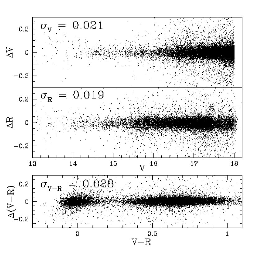
Figure 5: The differences in $V$, $R$, and $(V-R)$ for stars in field-overlap regions are plotted as a function of magnitude or color in the top, middle, and bottom panels respectively. Approximately 20,000 stars are plotted, each have $V\lower 2.15277pt\hbox{$\,\buildrel<\over{\sim}\,$}$ 18 mag and are located in 150 chunks tying together 21 of the LMC top-22 fields. The pair-wise comparisons of overlapping chunk photometry are plotted in no particular order in a global sense, but all chunk pairs connecting the same two fields have been subtracted in the same order. Standard deviations, as described in the text and illustrated here, are labeled in each panel. These values indicate the precision of the calibrated MACHO photometry for $\sim$9 million stars distributed over 10 square degrees of the LMC bar.

The MACHO calibrations have an internal precision of $\sigma_{V}$ = 0.021 mag, $\sigma_{R}$ = 0.019 mag, and $\sigma_{V-R}$ = 0.028 mag for $\sim$9 million stars distributed over $\sim$10 square degrees of sky. This is illustrated in Figure 5 where we plot $\sim$20,000 stars in 150 chunks with $V<18$ mag. We plot the offset in $V$, $R$, and $(V-R)$ versus magnitude or color in the top, middle, and bottom panels respectively. The standard deviations given above (and labeled in Figure 5) are calculated from the median offsets determined for each of the 150 field-overlap chunk pairs.

4 Comparisons with Other Photometry

4.1 Ground-based Data

It is customary to compare newly calibrated photometry with previously published data. We have arbitrarily selected $\sim$200 stars representing photographic, photoelectric, and CCD data from a dozen different authors. This may be a representative sample. We restrict this comparison to our $V$ photometry, because $R$ photometry is less common. In §4.2, we make comparisons with our $V$ and $R$ calibrated photometry, which allows the reader a more comprehensive assessment of the data.

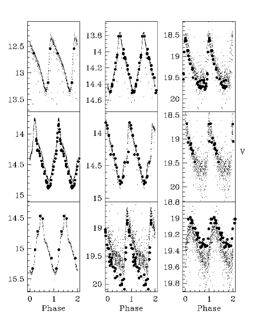
Figure 6: Period-folded MACHO $V$ lightcurves compared with photometry data assembled from the literature (5 different sources). MACHO data are plotted as dots and the comparison data as filled circles. Error bars are omitted for clarity. From top to bottom then left to right the variables are Cepheids: HV900, HV905, HV2510, HV2352, HV2324, and RR Lyrae near the cluster NGC 1835: GR-6 GR-14, GR-16, and Walker-V26. See text for further details.

We begin with a comparison of nine period-folded $V$ band lightcurves for an arbitrary sample of RR Lyrae and classical Cepheid variables. In Figure 6, from top to bottom then left to right we plot the classical Cepheids: HV900, HV905, HV2510, HV2352, and HV2324, and the RR Lyrae near the cluster NGC 1835: GR-6, GR-14, GR-16, and Walker-V26. The MACHO data consists of $\sim$1000 measurements; they are plotted as dots. Error bars are omitted for clarity. The comparison data are plotted as filled circles and are assembled from Martin and Warren (HV900, HV2323, HV2352; 1979), Sebo and Wood (HV905; 1995), Martin (HV2510; 1981) and from Walker (the RR Lyrae; 1993). For the RR Lyrae, the finding charts from Graham and Ruiz (1974) were also employed. We note that the photometry of Moffett et al. (1998; not plotted) for HV900 also shows satisfactory agreement with the MACHO data. All of the RR Lyrae are located in the same MACHO field and chunk, thus the $\sim$0.2 mag differences in brightness from star to star may not be attributed to a calibration error. These RR Lyraes illustrate the difficulty obtaining accurate photometry in crowded fields at this brightness.

In Figure 7, we compare our $V$ photometry with various other data. We plot $\delta V$(MACHO$-$Other) versus $V$ mag. We designate different author’s data with different symbols as follows. Asterisks are the Cepheids and RR Lyrae from Figure 6, filled circles are Walker’s (1993) standard star sequence near NGC 1835, open triangles are standard sequence of Cowley et al. (1990) near Cal-87 (finding chart found in Pakull et al. 1988), filled triangles are data from Flower et al. (1982) near NGC 2058/2065, open squares are stars near NGC 1847 from Nelson and Hodge (1983), and the open circles are photometry assembled from the classical LMC bar photometry paper by Tifft and Snell (1971). The median offset between MACHO and all of the other data is $\delta V=-0.035$ mag, which is indicated with a dashed line. Differences among the various authors likely represent systematic calibration errors.

4.2 HST Data

We have obtained Hubble Space Telescope (HST) Wide Field Planetary Camera (WFPC2) image data with the F555W and F675W filters for three fields in the LMC top-22. These are located in the field-overlap region of MACHO fields 2 & 79, in field 13, and in field 11. The reader is referred to Alcock et al. (1997) for a map and sky coordinates of these fields. For each field, we obtained “shorts” (3-4 $\times$ 30 sec exposures) and “longs” (3-4 $\times$ 400-500 sec exposures), in both filters.

Complete details of the HST data reduction and analysis will be presented elsewhere (Nelson et al. 1999). Briefly, the images were co-added and geometrically corrected with the aid of the stand-alone Drizzle package (Fruchter & Hook 1998). We performed aperture photometry with the centroids accurately determined via PSF fitting using Allstar II/Allframe and Daophot II (Stetson 1987, 1990). Stars were matched between filters for the longs and shorts separately, and for each field observed. Only stars identified in both colors were kept in the final photometry lists. The median aperture correction was calculated from $\sim$50 bright and isolated stars per WF chip, per short or long exposure, and per filter. The photometry lists were calibrated according to Holtzmann et al. (1995) using the coefficients in their Table 7 and the bay 4 gain ratios. The short and long photometry lists were then combined, including all stars found in either list, and adopting the long exposure magnitudes for stars in common to both lists. We made no correction for the WFPC non-linearity.

In Figures 8, 9, and 10 we compare approximately 120 stars identified in both the MACHO and HST photometry data. For each field we show the difference in magnitude, $\delta V$ and $\delta R$ (MACHO $-$ HST), as a function of $V$ or $R$ (top two panels) and $\delta(V-R)$ versus $(V-R)$ in the bottom panel. The open triangles are data from the WF2, the open circles are from WF3, and the open squares are from WF4. The median offset of the data is labeled in each panel. Typical dispersion about these median offsets is 0.02 mag. A direct comparison of ground-based and HST data is complicated by the radically different resolutions. We have simply added the flux for all HST stars inside a 1” radius of the star identified as the match to the MACHO object. Various trials with different “artificial blending” schemes indicate that the precision of this comparison is $\sim$0.05 mag. It is difficult to identify the magnitude and angular separation (among pairs or groups of stars) where the faint HST stars “become sky” and would no longer be counted in the ground-based SoDOPHOT measurements. Resolution of this issue is beyond the scope of this work.

The MACHO and HST photometry comparisons in Figures 8-10 show agreement at the $\sim$5% level or better. We note that there are no systematic differences between the photometry derived for the three WF CCDs and the MACHO photometry (in each case, derived from a single CCD image), in three separate comparisons. Our fields are particularly useful for this comparison, because they are fairly uncrowded (for HST) and the comparison stars are distributed throughout each WF CCD, in each field. The apparent consistency of the calibrated WF photometry supports the procedure we have used for calculating the aperture corrections and also supports the calibration formulae for WFPC2 given by Holtzmann et al. (1995). Given the $\sim$5% uncertainty associated with blending the HST data to match the MACHO data, these comparisons indicate that $R$ agrees quite well, and that the calibrated colors are offset by 0.04 mag ($(V-R)_{HST}\approx(V-R)_{MACHO}+0.04$).

In Figure 11, we present two side-by-side CMDs showing the 120 MACHO objects and the “un-blended” HST photometry from the comparison above. We plot the MACHO objects in the left panel and the HST stars in the right panel. Without making any corrections for completeness in the HST data, this naive comparison yields a star to object ratio $S/O$ = 229/120 = 1.91. This value is sensitive to the adopted match radius (1”), but may reasonably be considered a lower limit to the average star to object ratio in these three fields. We will return to this in §7.

5 Other MACHO Fields

5.1 Bulge Field 119 and SMC Field 207

We have calculated calibration zero-points for field 119 (Baade’s Window) in the Galactic bulge and field 207 (near the cluster NGC 330) in the SMC by matching published photometry to MACHO data.

MACHO field 119 is centered on Baade’s Window. Calibrated photometry of $\sim$70 stars from Cook (1986) and 7 standard stars from Walker and Mack (1986) in the $V$ and $I$ passbands were converted to $V$ and $R$ using $(V-R)=0.50(V-I)$ (e.g. Landolt 1992). These stars were then identified in the MACHO photometry database. The MACHO photometry was corrected for color and airmass according to equations (1) & (2) of this paper. Chunk offsets were assumed to be zero everywhere. In Figure 12, we plot the difference between the standard and color corrected instrumental MACHO magnitudes as a function of $V$ mag. The same plot is shown in the bottom panel for the $R$ mags. The median values of these magnitude differences are our adopted solutions for $a0$ and $b0$, and are plotted as solid lines in the top and bottom panels respectively. The zero-points are $a0=18.259$ and $b0=17.972$, with a standard deviation of $\sim 0.025$ mag.

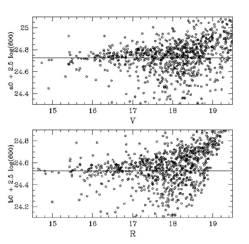
Figure 13: The solution for $a0$ and $b0$ using the published photometry of Vallenari et al. (1994) in MACHO SMC field 207.

The well-studied SMC cluster NGC 330 is located in MACHO field 207. We have used photometry from Vallenari et al. (1994) near NGC 330 to calibrate our SMC photometry. These data are in $B$ and $V$ and we have converted them to $V$ and $R$ using $(V-R)=0.56(B-V)$. The MACHO instrumental photometry was corrected for the color and airmass according to equations (1) & (2). We plot the data used for the field 207 zero-point solutions in Figure 13. We find $a0=17.788$ and $b0=17.584$, with a standard deviation of $\sim$0.07 mag; these are indicated with solid lines in Figure 13.

5.2 Status of Calibration for All Other MACHO Fields

In Figure 14 we plot the LMC top-22 zero-points ($a0$ top panel, $b0$ middle panel, and $a0-b0$ in the bottom panel) as a function of template airmass ($X_{t}$) using small open circle symbols. The single bulge zero-point is plotted with a filled circle symbol, and the single SMC zero-point is plotted with a filled triangle symbol. Linear regressions of the LMC top-22 zero-point data are indicated with dashed lines in each panel. We will use these to predict approximate zero-points for all other MACHO fields in the LMC, SMC, and bulge. The derived regressions are,

$$a0=18.410-0.279X_{t}$$ (3)

$$b0=18.087-0.222X_{t}$$ (4)

The uncertainty in the zero-points are $\pm 0.06$ and the uncertainty in the slopes are $\pm 0.04$. The dispersion of the data about each of these regressions is $\sim$0.10 mag. The datapoints lying below the regressions are likely due to non-photometric conditions (i.e. clouds), while the points above tend to have good seeing (this represents a by-field aperture correction, relative to the typical observation). At this time, the calibration zero-point uncertainty for all fields in the MACHO database which have not been explicitly calibrated in this paper is 0.10 mag. The uncertainty in color is 0.04 mag, which is estimated from the dispersion about the $a0-b0$ regression in the bottom panel of Figure 14.

6 Lightcurve Calibration

6.1 Blue Jitter

MACHO instrumental lightcurves in the blue show a systematic source of scatter which is directly attributable to the responses of the different Loral CCDs and a secondary focal plane position-dependent effect likely due to the dichroic. This is blue jitter. Because observations of LMC and SMC fields are made from both sides of the pier, stars will alternatively land on the CCDs rotated 180 degrees from each other in the focal plane (i.e. a star will land in CCDs 4 & 6, or 5 & 7 depending on pier side). The opposite-pier side template photometry is modified (i.e. the template photometry is “jittered”) so that PSF fitting in SoDOPHOT will converge quickly. This has the effect of maintaining the systematic differences in blue photometry derived from different pier side observations in the resulting instrumental lightcurves. It is possible to “de-jitter” lightcurves by applying the inverse of the template photometry blue jitter correction. The de-jitter algorithms have the form,

$$V_{M,t}=V_{M,e}+BJ_{e}\ \left[\left(V_{M,e}-R_{M,e}\right)-BJ_{o}\right]$$ (5)

$$V_{M,t}=V_{M,w}+BJ_{w}\ \left[\left(V_{M,w}-R_{M,w}\right)-BJ_{o}\right]$$ (6)

where the subscripts “e” and “w” stand for East and West respectively. The subscript “t” stands for template magnitude; thus $V_{M,t}$ calculated from equations (5) & (6) is an appropriate magnitude for input into equations (1) & (2). De-jitter corrections require an instrumental color for each measurement. They also require the three coefficients $BJ_{e}$, $BJ_{w}$, and $BJ_{o}$.

The coefficients $BJ_{e}$ and $BJ_{w}$ depend on (red West of pier) chunk and field. The field gives the style template, and the chunk specifies location in the focal plane. The coefficients $BJ_{e}$ and $BJ_{w}$ are unique for each chunk and applicable to all fields. However, the sign of the coefficient flips depending on the style template, and for every chunk, either $BJ_{e}$ or $BJ_{w}$ is set equal to zero. The $BJ_{w}$ coefficients in Figure 15 are for blue jitter corrections in the imaginary case of a West of pier observation made of a field with template photometry derived from an entirely East of pier observation. This illustrates the focal plane dependence.

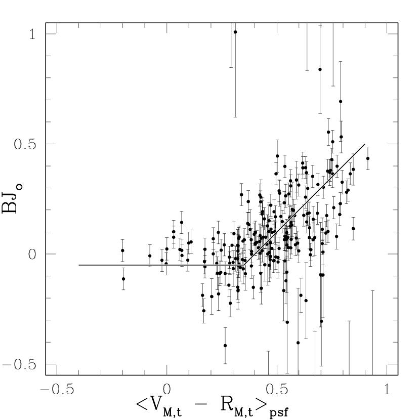
Figure 16: Data for 224 chunks in 5 different LMC fields used to derive the $BJ_{o}$–(mean color of PSF stars) calibration for the blue jitter corrections. The solid line is the adopted calibration.

The coefficient $BJ_{o}$ is unique to every field and chunk, and is calculated from the mean color of the PSF stars in that chunk. $BJ_{o}$ is simply the color in each chunk where no blue jitter correction is necessary. The calibration between $BJ_{o}$ and the mean color of the PSF stars in a chunk was derived by minimizing the difference of mean blue magnitudes calculated using only East and West of pier data in the four-year lightcurves of $\sim$400 constant brightness stars (per chunk), for 224 different chunks in 5 different LMC fields (9, 10, 18, 19, 82). These data are shown in Figure 16 along with our adopted calibration (shown as a solid line), which follows: for mean PSF colors $(V-R)_{\overline{PSF}}$ $<$ $0.35$ mag the coefficient $BJ_{o}$ = $-0.05$ and for $(V-R)_{\overline{PSF}}$ $>$ $0.35$ mag the coefficient $BJ_{o}=-0.4$ + $(V-R)_{\overline{PSF}}$. We estimate that de-jittering will be accurate to $\pm 0.02$ mag with this procedure. The mean color of the PSF stars has been calculated for every chunk in the MACHO database.

6.2 Color Airmass

MACHO instrumental lightcurves may show systematic changes in brightness which are correlated with the airmass of individual observations. Due to the limited observing season and the high priority set for observing the LMC, these fields are observed at progressively higher airmasses as the season progresses. This may result in slow “seasonal rolls” ($\sim$1 year periods) in some instrumental lightcurves. We present here an algorithm for an airmass and color-dependent lightcurve correction. This correction is not implemented in any existing MACHO calibration code, but may potentially be useful for correcting small numbers of astrophysically interesting lightcurves.

The color airmass corrections should be made on East and West of pier lightcurve data separately before making blue jitter corrections. We show the form of the correction for East of pier data, maintaining the use of the subscript “e” to designate these measurements. The correction is equally applicable to the West of pier data. We designate the $raw$ magnitudes with a prime symbol. The color airmass corrected data does not have the prime, and would be appropriate for substitution into equations (5) & (6) for blue jitter corrections. The color airmass corrections have the form,

$$V_{M,e}=V_{M,e}^{{}^{\prime}}+0.033\ \left(X-X_{t}\right)\ \left[\left(V_{M,e}^{{}^{\prime}}-R_{M,e}^{{}^{\prime}}\right)-CA_{o}\right]$$ (7)

$$R_{M,e}=R_{M,e}^{{}^{\prime}}+0.006\ \left(X-X_{t}\right)\ \left[\left(V_{M,e}^{{}^{\prime}}-R_{M,e}^{{}^{\prime}}\right)-CA_{o}\right]$$ (8)

where $X$ is the airmass of each observation, $X_{t}$ is the airmass of the template observation, and $CA_{o}$ is the color for which no airmass-correlated changes in brightness are observed. The ratio of the color airmass coefficents in equations (1) & (2) to the color airmass coefficients given in equations (7) & (8) are $V$: 0.022/0.033 and $R$: 0.004/0.006. Both ratios are $\sim$0.66, which is approximately $(V-R)$/$(V_{M}-R_{M})$. These color airmass coefficients are derived from MACHO instrumental lightcurves, and support the values used in the calibration formulae, i.e equations (1) & (2).

The $CA_{o}$ coefficient varies from chunk to chunk, although no correlation was found with the mean color of the PSF stars, as was the case for the blue jitter $BJ_{o}$ coefficient. Therefore, in order to make the color airmass lightcurve correction, $CA_{o}$ must be derived using separate knowlege of the shape of a lightcurve. For example, one could solve for $CA_{o}$ by minimizing the scatter in the period-folded lightcurve of a Cepheid variable star. An alternative way to solve for $CA_{o}$ would be to minimize the scatter in several constant brightness stars in the same chunk as the star of interest. In this case, it is recommended that several nearby stars are used in the solution, and that they have a wide range in colors, ideally bracketing the color of the star of interest. It is recommended to inspect scatter plots of $V_{M,e}$-$X$ and $V_{M,w}$-$X$ (separately, as blue jitter may mask the effect) in order to estimate the degree to which any particular lightcurve is affected.

6.3 Other Systematic Lightcurve Effects

We offer a few cautionary remarks to potential users of MACHO data. (1) Weather permitting, the MACHO Project will observe every night of the year. This includes nights when the seeing (the FWHM of the stellar PSF) approaches $\sim$7 arcsec. In our typically crowded fields, poor seeing can lead to inaccurate photometry, despite the small photometric uncertainties that may be reported by SoDOPHOT. Inspection of scatter plots of $V_{M,w}$- and $V_{M,e}$-$Seeing$ are useful diagnostics for this source of systematic lightcurve scatter. This so-called “seeing variability” can be quite large (easily a few tenths of a magnitude), particularly for very crowded stars or stars nearby to regions of irregular, bright nebulosity. It is not recommended to globally decorrelate lightcurves with seeing. (2) The catalogs of CCD defects polluting the MACHO focal plane are not perfect. Uncataloged CCD defects will cause spurious photometric measurements, which are not necessarily reflected in the photometric uncertainty or integer flags reported by SoDOPHOT. In this case, inspection of the image data is very useful. (3) In some cases, lightcurves will exhibit additional scatter over that expected from the uncertainties of individual measurements which is not attibutable to any of the aforementioned effects. This may be due to the inclusion of variable stars in the PSF fiducial lists used by SoDOPHOT. In this case, other lightcurves in the same chunk may also be affected.

7 The Efficiency CMD

The efficiency calculation will be reported in complete detail elsewhere (Alcock et al. 1999). Briefly, the calculation is a massive series of artificial star tests with raw image data spanning four years of observations followed by Monte-Carlo experiments to detect fake microlensing events in accurately simulated artifical datasets. The efficiency calculation returns our sensitivity to detect microlensing in stars (not “objects”, see §1). We calculate the star to object ratio in the MACHO data by comparing with the HST data. We assume that there are no objects in the high resolution image data from the HST, only real stars .

The efficiency CMD represents real LMC stars and contains accurate information on their surface density as a function of color and magnitude. For convenience, we use an area normalization of 0.52 square degrees (one MACHO field). The limiting magnitude of the efficiency CMD is set by the faintest LMC star for which we may realistically detect microlensing. We adopt $V$ = 25 mag, indicated by preliminary results from the efficiency Monte-Carlos. The efficiency CMD plays two roles in the efficiency calculation: (1) it is used to seed the artificial star tests with stars drawn from a realistic distribution in color and brightness, and (2) the derived efficiency (for stars) must be integrated over the efficiency CMD to calculate the efficiency per object in the MACHO database. The required accuracy of the efficiency CMD is dictated by the second application. The efficiency CMD has direct consequences for our measurement of the LMC microlensing optical depth.

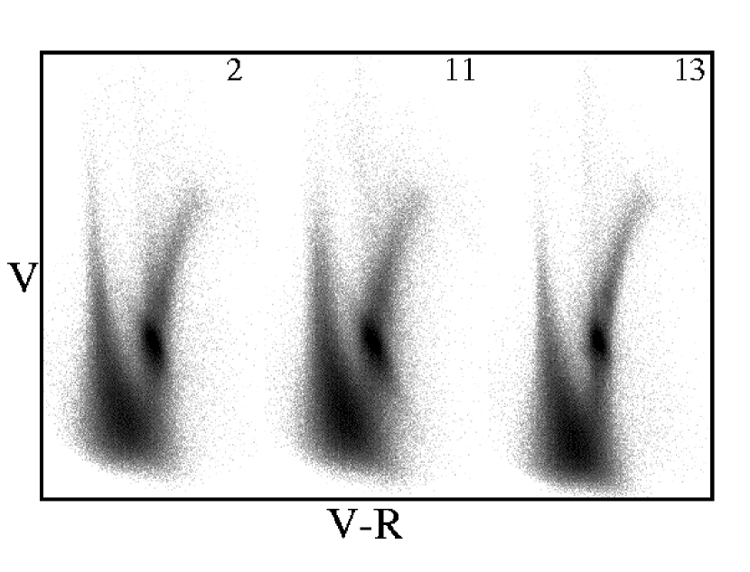
Figure 17: MACHO calibrated Hess diagrams for LMC fields 2, 11, and 13. Although axes are not labeled, for each field they run from $(V-R)=-0.5$ to 1.5 mag (bin size 0.01 mag), and $V=22$ to 14 (bin size 0.02). Intensity represents the number of stars. The diagrams have been log-scaled. These diagrams allow a qualitative comparison of the CMDs for each field.

In Figure 17, we compare the three MACHO CMDs for fields 2, 11, and 13 for which we also have HST data (these are actually log-scaled Hess diagrams). Fields 2, 11, and 13 contain 354586, 426060, and 344746 objects respectively. We note that field 13 has the faintest limiting magnitude. Also, with the exception of the varying degree of differential reddening (field 11 is the most affected), and slight differences in the numbers of upper-main sequence stars, these three CMDs are quite similar.

In Figure 18, we compare the MACHO object luminosity functions with the HST star luminosity functions (LFs). We plot $dN/dV$ as a function of $V$ mag. The units of $dN/dV$ are $10^{4}$ stars (or objects) per 0.52 square degree in 0.125 $V$ mag bins. The MACHO data are shown as solid lines. The HST data are shown as open circles connected by dotted lines. The typical error bar for the HST data is indicated in the upper right corner. We compare fields 2, 11, and 13 in the top, middle, and bottom panels, respectively. The HST data has been scaled to the MACHO data by a factor of 409, which is estimated as follows. The effective area photometered for each HST field is is $3\times 747.5\times 747.5$ pixels. The plate scale of 0.”1/pix yields a sky area of 4.6 square arcmin per field. The MACHO plate scale of 0.”635/pix, and mosaic of $4\times 2048\times 2048$ Loral CCDs yields a total sky area of 1879.1 square arcmin per field. We scale the HST data by the ratio of sky areas after making a small (2%) correction for completeness in the HST data (see below). Figure 18 shows that the MACHO photometry is incomplete at the brightness of the red horizontal branch clump ($V\sim 19.3$ mag) in fields 2 and 11. In constrast, field 13 appears complete to $V\sim 21$ mag.

In Figure 19, we compare the HST LFs for the three fields. We plot the logarithm of $dN/dV$ (same units as in Figure 18) as a function of $V$ mag. Fields 2, 11, and 13 are shown as dotted, short-dash, and long-dash lines respectively. The sum of these three LFs is shown as a bold line. Preliminary artificial star tests indicate that we are $\sim$ 98% complete to $V\sim 22$ mag. We have fit a power-law to the summed LF in the magnitude range $V=19.5$ to 22 mag, and extended it to $V$ = 25 mag (the slope of the derived power-law is $\alpha=0.415\pm 0.017$). The power-law LF is shown as a solid line. We assume this closely approximates the true LF. Deviations from the power-law may be dues to incompleteness in the HST data or reflect a real turn-over. We will use (below) the ratio the power-law LF to the summed HST LF to re-scale the number of stars in the efficiency CMD from $V$ = 22 to 25 mag. Considering only stars with $V<25$, the summed HST LF contains 17006732 stars. The summed HST LF for $V<22$ plus the power-law LF for $22<V<25$ contains 55864940 stars.

In order to improve the sampling of the sparsely populated bright end of the efficiency CMD, we will “splice” the bright MACHO data to the faint HST data. We will make the splice at $V=18.7$ mag, where brighter than this, all three MACHO fields appear to be complete (see Figure 18). The HST data and the MACHO data for the three fields are each binned in color from $(V-R)$ = $-0.5$ to 1.5 in bins of 0.05 mag and in brightness from $V$ = 25 to 15 in bins of 0.10 mag. These 2-d histogram data are converted to images compatibile with IRAF. Within IRAF, we replace all pixels fainter than $V$ = 18.7 mag in the MACHO CMD image with zero values, and similarly edit the HST image pixels values brighter $V$ = 18.7 mag. We additionally replace low density pixels with zero-values in each image. This step typically “removes” the few pixels containing galaxies, foreground stars, or bad measurements. In the HST image, these pixels would otherwise be scaled to very high values in the efficiency CMD. In the MACHO image, this step also removes features such as the upper-main sequence, asymptotic giant branches, supergiants, and foreground Galactic disk stars. The regions of the CMD populated by these features are excluded in the searches for microlensing anyway. This editing has a negligible effect on total number of stars in the efficiency CMD.

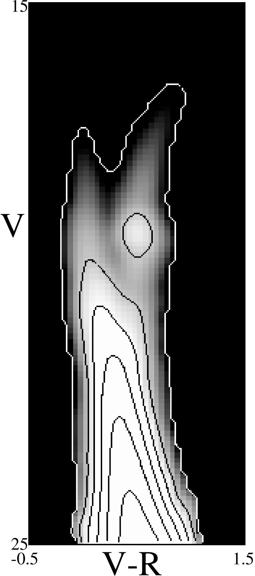
Figure 20: The efficiency CMD; a Hess diagram (2-d histogram) representing the number of stars per 0.52 square degrees in the LMC as a function of $V$ and $(V-R)$. Intensity represents the number of stars. Logarithmic contours are overplotted in the diagram. The lowest contour (white) represents 1.0 dex stars (per $\Delta(V-R)=0.05$, $\Delta V$ = 0.10 mag bin, and 0.52 square degree) while the other contours run from 3.5 to 5.5 dex in steps of 0.5 dex.

Next, we sum the edited HST and MACHO images and smooth the resulting image. We multiply the spliced and smoothed CMD image by a power-law scaling image. The resulting efficiency CMD is shown in Figure 20. Intensity represents the number of stars. The image is log-scaled; contours indicate 1.0, 3.5, 4.0, 4.5, 5.0, and 5.5 dex. The total number of stars represented is 55426384 (per 0.52 square degrees). The corresponding number of MACHO objects is 1125392, which yields a star to object ratio $S/O$ = 49.2 to $V$ = 25. We find $S/O$ = 1.2, 3.4, and 21.8 to $V$ = 20, 22, and 24 mag respectively. These values are systematically uncertain at the $\sim$8% level, depending on the counting of MACHO objects identified only in one color.

It may be possible to adopt a single efficiency CMD for the entire LMC and then use the efficiency Monte-Carlos to sort-out our relative sensitivities to detecting microlensing in different fields. However, we may also assess the uncertainty associated with the single efficiency CMD approximation as follows. Consider the three HST LFs in Figure 19. While the overall distributions are quite similar, fields 2, 11, and 13 contain 1335794, 1406142, 595913 stars (scaled to 0.52 square degrees) with $V<22$ mag. Using the total number of MACHO objects in these fields, we find $S/O$ = 3.8, 3.3, and 1.7 for fields 2, 11, and 13 respectively, which yields $<S/O>=2.9\pm 1.0$. The standard deviation indicates the uncertainty of our single efficiency CMD approximation. Because of the power-law LF corrrection for $V>22$ mag, $S/O$ to all fainter magnitudes scales directly from the $V\sim 21$ mag portion of the HST LFs.

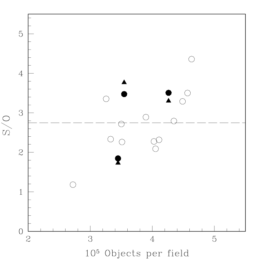
Figure 21: Star/Object ratio (S/O) to the limiting magnitude $V$ = 22 for 16 fields near the LMC bar as a function of the number of MACHO objects per field. Solid triangles are calculated from HST/MACHO photometry comparisons for three fields (see text). Solid circles show the fit values to a regression of these three S/O values and surface brightness measurements. The open circles show the S/O ratios predicted by the surface brightness regression for an additional 13 MACHO LMC fields.

We may extend this analysis to other fields using surface brightness measurements in the LMC. First, we measure relative fluxes (arbitrary units) for 16 MACHO fields from the Bothun and Thompson (1988) “Parking Lot Camera” wide-field R-band image of the LMC (the fields and this image are shown in Fig. 1 of Alcock et al. 1997). We exclude the central-most bar fields because the image is saturated here. We also exclude two fields near 30 Doradus. The 16 fields selected span the “middle range” of the 30 fields targeted for the upcoming LMC microlensing analysis in terms of total number of objects. For our three fields with HST data, we perform a linear regression between the HST-derived $S/O$ ratios and their surface brightnesses. We then use surface brightness to predict $S/O$ for the remaining fields. These data are shown in Figure 21 where we plot $S/O$ as a function of total number of objects per field (in units of $10^{5}$ objects). Filled triangles are the $S/O$ values calulated from the HST data for fields 2, 11, and 13. The filled circles are the fit values from the surface brightness regression for these three fields. The open circles are the estimates $S/O$ values for the remaining fields. We are primarily concerned with the estimated scatter; the standard deviation is $\sim$0.80, or a 30% uncertainty in $S/O$ (also labeled on Figure 21).

Figure 21 suggests a correlation between $S/O$ and total number of MACHO objects per field. It may be the case that additional parameters (i.e. seeing or sky in the template images) would improve the correlation. If so, such a correlation may be used to rescale the efficiency CMD and improve the accuracy of the efficiency calculation, particularly as a function of position in the LMC. However, this analysis awaits further characterization of our SoDOPHOT-derived photometry and the efficiency Monte-Carlo results.

8 Summary

In this paper, we have described MACHO Project photometry data and calibration of these data. We have transformed our two-color instrumental photometry for $\sim$9 million stars in the LMC top-22 fields (Alcock et al. 1997) to the Kron-Cousins $V$ and $R$ system with a precision of $\sigma_{V}=0.021$, $\sigma_{R}=0.019$, and $\sigma_{(V-R)}=0.028$ mag. The uncertainties associated with the CTIO photometry aperture corrections and the MACHO transformation zero-points are the most significant for the overall accuracy of the photometric calibration. We estimate $\pm 0.018$ for the former, and $\pm 0.03$ mag for the latter, which is likely a correlated error in $V$ and $R$. Therefore, we estimate the overall accuracy of these calibrated MACHO photometry to be $\pm 0.035$ mag in $V$, $R$, and $(V-R)$. This appears consistent with comparisons of calibrated MACHO photometry data to published photometric sequences and calibrated HST observations. The accuracy of the calibrated MACHO photometry may be worse for stars with extreme colors due to our non-standard passbands. Calibration for all fields not including the LMC top-22 (Alcock et al. 1997), SMC field 207, and Galactic bulge field 119 has a zero-point uncertainty of 0.10 mag and a color uncertainty of 0.04 mag. The calibration presented in this work supersedes all prior calibration of MACHO photometry in the LMC, SMC, and Galactic bulge.

The detailed descriptions of the data reduction and photometry database provided in this work are largely intended to guide consumers of released MACHO data. If potential calibrators have assembled MACHO instrumental template photometry, or otherwise adopted/calculated MACHO instrumental magnitudes and colors as substitutes for the original template photometry, the necessary calibration formulae are given in §3.1. We have additionally discussed the calibration of MACHO lightcurves. If potential calibrators will make detailed analyses of MACHO lightcurves, they should consider making corrections for known systematic effects such as blue jitter (§6.1), color-dependent airmass variability (§6.2), as well as effects due to seeing and uncatalogued focal plane defects (§6.3). Last in this work, we have described the construction of the efficiency CMD, a cornerstone of the new microlensing detection efficiency calculation, which will be presented in a forthcoming MACHO collaboration paper.

9 Acknowledgements

David Alves thanks his graduate advisors, Kem Cook and Robert Becker, for their support. We thank the skilled support by the technical staff at MSSSO. Work at LLNL supported by DOE contract W7405-ENG-48. Work at CfPA supported by NSF AST-8809616 and AST-9120005. Work at MSSSO supported by the Australian Dept. of Industry, Technology and Regional Development. WJS thanks PPARC Advanced Fellowship, KG thanks DOE OJI, Sloan, and Cottrell awards, CWS thanks Sloan and Seaver Foundations.

1cm

Table 1: SODOPHOT Integer Flags

i-type	meaning
1	bright, unsplit star
2	bright, split star
3	faint, unsplit star
4	faint, split star
5	very faint or unconverged unsplit star
6	very faint or unconverged split star
7	too faint or off the image, unsplit star
8	too faint or off the image, split star
9	unconverged in 7 parameter fit
10	large number of pixels missing ($>$ 35%)
11	cosmic ray
12	galaxy (currently disabled)
13	obliterated star

1cm

Table 2: Calibration Color Coefficients

Blue CCD No.	$a1$	Red CCD No.	$b1$
1	$-0.1876$	6	0.1868
2	$-0.2065$	5	0.1784
3	$-0.2059$	4	0.1784
0	$-0.2059$	7	0.1784

Figure 1: Approximate instrumental throughput for the blue and red MACHO image data. A throughput of one would indicate no loss of light; wavelength is in units of $nm$. These response functions include the dichroic, filters, and CCDs. However, the wide-field optics corrector has not been included. Uncertainty in these functions is $\sim$20%. Also shown are normalized standard passbands $B$, $V$, $R$ and $I$.

Figure 2: Schematic of of the MACHO focal plane (red left, blue right) in the East of pier (top) and West of pier (middle) orientation. CCD-Amplifier combinations are labeled. The inoperational amplifier 0.0 is marked with an X. The bottom two panels are the chunk maps of the red (left) and blue (right) MACHO focal planes in the West of pier orientation. Chunks are always fixed to the same CCD-Amplifier. Thus, the chunk map rotates 180^∘ when in the East of pier orientation.

Figure 3: CTIO and MACHO calibration data for the four zero-point chunks in LMC field 13. The left panel shows the CTIO calibration data in the CMD; approximately 2500 stars are plotted. The difference in calibrated MACHO and CTIO photometry ($\delta V$ and $\delta R$) as a function of $V$ and $R$ mag are plotted in the middle and right panels, respectively.

Figure 4: Mean chunk offsets calculated for the top-22 field LMC calibration labeled on a chunk map to illustrate the focal plane dependence. Listed in each of the 64 chunk locations is mean chunk offset (upper left number), and red West of pier chunk number (lower right number). See also Figure 2.

Figure 7: MACHO calibrated $V$ photometry in the LMC compared with various published measurements. The data are represented by the following symbols: asterisks are the Cepheids and RR Lyrae from Fig. 6, filled circles are Walker’s standard star sequence near NGC 1835 (1993), open triangles are standard sequence of Cowley et al. (1990) near Cal-87, filled triangles are data from Flower et al. (1982) near NGC 2058/2065, open squares are stars near NGC 1847 from Nelson and Hodge (1983), and the open circles are photometry assembled from the classical LMC photometry paper by Tifft and Snell (1971). The median offset between the MACHO and all of the other data is indicated with a dashed line.

Figure 8: MACHO calibrated photometry for field 2 compared with HST calibrated photometry. Open trangles are data from the WF2 chip, open circles from WF3, and open squares from WF4. We plot the magnitude or color offset, $\delta V$, $\delta R$, and $\delta(V-R)$, in the sense (MACHO - HST) versus magnitude or color. The median offset is labeled in each panel.

Figure 9: Same as Fig. 8, but for MACHO field 11.

Figure 10: Same as Fig. 8, but for MACHO field 13.

Figure 11: Color-magnitude diagrams showing the MACHO objects and (un-blended) HST stars from Figures 8-10. Each panel is labeled. The ratio of stars to objects is 229/120 = 1.91, also labeled.

Figure 12: The solution for $a0$ and $b0$ using the published photometry of Cook (1986) and Walker and Mack (1990), plotted as open and filled circles respectively, in MACHO bulge field 119.

Figure 14: Calibration zero-points ($a0$ and $b0$) for the top-22 LMC fields (open circles), Galactic bulge field 119 (filled circle), and SMC field 207 (filled triangle) plotted as a function of template airmass, $X_{t}$. Dashed lines show the regressions used to predict the calibrations zero-points for all other MACHO fields.

Figure 15: Blue jitter $BJ_{w}$ coefficients labeled on a chunk map to illustrate the focal plane dependence. Center in each of the 64 chunk locations is $BJ_{w}$ while the red West of pier chunk number is the lower right number (see also Figure 2). These coefficients are for blue jitter corrections in the imaginary case of a West of pier observation made of a field with template photometry derived from an entirely East of pier observation.

Figure 18: Luminosity functions for LMC fields 2, 11, and 13 comparing MACHO and HST data. The HST data has been scaled to the MACHO data. The typical errorbar associated with each bin of HST data is indicated in the upper right corner.

Figure 19: Luminosity functions for LMC fields 2, 11, and 13 comparing HST data. The units of $dN/dV$ are as in Fig. 18. The sum of the three HST LFs is a bold line. Power-law fit and extension is solid line (see text).

References

- (1)
- (2) Alcock, C. et al. (MACHO), 1997, ApJ, 486, 697
- (3) Alcock, C. et al. (MACHO), 1999, in prep.
- (4) Axelrod, T. et al. (MACHO) 1998, SPIE, 3349, 152
- (5) Bessell, M. 1979, PASP, 91, 589
- (6) Bessell, M. 1986, PASP, 98, 1303
- (7) Bessell, M. 1987, PASP, 99, 642
- (8) Bessell, M. 1990, PASP, 102, 1181
- (9) Bessell, M. 1995, PASP, 107, 672
- (10) Bothun, G.D., & Thompson, I.B. 1988, AJ, 96, 877
- (11) Cook, K. 1986, Ph.D. dissertation, Univ. Arizona
- (12) Cowley, A. et al. 1990, ApJ, 350, 288
- (13) Flower, P. 1982, PASP, 94, 894
- (14) Fruchter, S. & Hook R. 1998 in prep. (see also astro-ph/9808087)
- (15) Graham, J. 1982, PASP, 94, 244
- (16) Graham, J. & Ruiz, M. 1974, AJ, 79, 3
- (17) Groth, E. 1986, AJ, 91, 1244
- (18) Hart, J. et al. (MACHO) 1996, PASP, 108, 220
- (19) Holtzmann, J. et al. 1995, PASP, 107, 1065
- (20) Landolt, A.U. 1992, AJ, 104, 340
- (21) Marshall, S. 1994, Ph.D. dissertation, U.C. Santa Barbara
- (22) Martin, W.L. 1981, SAAOC 6, 96
- (23) Martin, W.L. & Warren, P.R. 1979 SAAOC 1, 98
- (24) Moffett et al. 1998, ApJS, 117, 135
- (25) Nelson, C.A. et al. 1999, in prep.
- (26) Nelson, M. & Hodge, P. 1983, PASP, 95, 5
- (27) Paczýnski, B. 1986, ApJ, 304, 1
- (28) Pakull, M. et al. 1988, A&A, 203, 627
- (29) Robinson, T. & Grubb, T. 1869, Philos. Trans. R. Soc., 159, 127
- (30) Schechter, P.L., Mateo, M., & Saha, A. 1993 PASP 105, 1342
- (31) Sebo, K. & Wood, P. 1995, ApJ, 449, 164
- (32) Stetson, P., 1987, PASP, 99, 191
- (33) Stetson, P., 1990, PASP, 102, 932
- (34) Stubbs, C. et al. (MACHO) 1993 Charge Coupled Devices and Solid State Optical Sensors III ed. Blouke, M. Proceedings of the SPIE, 1900
- (35) Tifft, W. & Snell, C. 1971, MNRAS, 151, 365
- (36) Vallenari, A., Ortolani, S. & Chiosi, C. 1994, A&AS, 108, 571
- (37) Walker, A. 1993, AJ, 105, 527
- (38) Walker, A. & Mack, P. 1986, MNRAS 220, 69
- (39)
1cm