The MHD Kelvin-Helmholtz Instability III:
The Role of Sheared Magnetic Field in Planar Flows

Abstract

We have carried out simulations of the nonlinear evolution of the magnetohydrodynamic (MHD) Kelvin-Helmholtz (KH) instability for compressible fluids in $2\frac{1}{2}$-dimensions, extending our previous work by Frank et al. (1996) and Jones et al. (1997). In the present work we have simulated flows in the $x-y$ plane in which a “sheared” magnetic field of uniform strength “smoothly” rotates across a thin velocity shear layer from the $z$ direction to the $x$ direction, aligned with the flow field. The sonic Mach number of the velocity transition is unity. Such flows containing a uniform field in the $x$ direction are linearly stable if the magnetic field strength is great enough that the Alfvénic Mach number, ${M_{A}}={U_{0}}/{c_{A}}<2$. That limit does not apply directly to sheared magnetic fields, however, since the $z$ field component has almost no influence on the linear stability. Thus, if the magnetic shear layer is contained within the velocity shear layer, the KH instability may still grow, even when the field strength is quite large. So, we consider here a wide range of sheared field strengths covering Alfvénic Mach numbers, ${M_{A}}=142.9$ to $2$.

We focus on dynamical evolution of fluid features, kinetic energy dissipation, and mixing of the fluid between the two layers, considering their dependence on magnetic field strength for this geometry. There are a number of differences from our earlier simulations with uniform magnetic fields in the $x-y$ plane. For the latter, simpler case we found a clear sequence of behaviors with increasing field strength ranging from nearly hydrodynamic flows in which the instability evolves to an almost steady Cat’s Eye vortex with enhanced dissipation, to flows in which the magnetic field disrupts the Cat’s Eye once it forms, finally, to flows that evolve very little before field-line stretching stabilizes the velocity shear layer. The introduction of magnetic shear can allow a Cat’s Eye-like vortex to form, even when the field is stronger than the nominal linear instability limit given above. For strong fields that vortex is asymmetric with respect to the preliminary shear layer, however, so the subsequent dissipation is enhanced over the uniform field cases of comparable field strength. In fact, so long as the magnetic field achieves some level of dynamical importance during an eddy turnover time, the asymmetries introduced through the magnetic shear will increase flow complexity, and, with that, dissipation and mixing. The degree of the fluid mixing between the two layers is strongly influenced by the magnetic field strength. Mixing of the fluid is most effective when the vortex is disrupted by magnetic tension during transient reconnection, through local chaotic behavior that follows.

1. Introduction

The Kelvin Helmholtz (KH) instability is commonly expected in boundary layers separating two fluids and should occur frequently in both astrophysical and geophysical environments. The instability taps the free energy of the relative motion between two regions separated by a shear layer, or “vortex sheet” and is often cited as a means to convert that directed flow energy into turbulent energy (e.g., Maslowe 1985). Astrophysically, the instability is likely, for example, along jets generated in some astrophysical sources, such as active galactic nuclei and young stellar objects (e.g., Ferrari et al. 1981). There are also strongly sheared flows in the solar corona (e.g., Kopp 1992). Geophysically, it is expected on the earth’s magnetopause separating the magnetosphere from the solar wind (e.g., Miura 1984).

The KH instability leads to momentum and energy transport, as well as fluid mixing. If the fluid is magnetized, then the instability can locally amplify the magnetic field temporarily by stretching it, enhance dissipation by reconnection, and lead to self organization between the magnetic and flow fields. The linear evolution of the KH instability was thoroughly studied a long time ago. The analysis of the basic magnetohydrodynamic (MHD) KH linear stability was summarized by Chandrasekhar (1961) and Miura & Pritchett (1982) and has been applied to numerous astrophysical situations (e.g., Ferrari et al. 1981; Bodo et al. 1998). Chandrasekhar showed, for example, that for incompressible flows, a uniform magnetic field aligned with the flow field will stabilize the shear layer if the Alfvénic Mach number of the transition is small enough; in particular, for a plasma of uniform density if $M_{A}=U_{0}/c_{A}<2$, where $U_{0}$ is the velocity change across the shear layer. There is now a considerable literature on the nonlinear evolution of the hydrodynamical (HD) KH instability (e.g., Corcos & Sherman 1984; Maslowe 1985) thanks to the development of both robust algorithms to solve fluid equations and fast computers to execute numerical simulations. However, the literature on the nonlinear behavior of the MHD KH instability is much more limited. That is because MHD physics is more complicated and because accurate, robust numerical algorithms, especially for compressible flows, are relatively new. Since a great many astrophysical applications surely involve magnetized fluids, it is important to come to a full understanding of the MHD version of the problem.

In the past several years initial progress has been made, especially in two-dimensional MHD flows involving initially uniform magnetic fields having a component aligned with the flow field (e.g., Miura 1984; Wu 1986; Malagoli et al. 1996; Frank et al. 1996 [Paper I]; Jones et al. 1997 [Paper II]). The KH problem is, of course, a study of boundary evolution. An interesting and physically very relevant variation on this problem adds a current sheet to the vortex sheet. Then, the direction and/or the magnitude of the magnetic field will change across the shear layer. Dahlburg et al. (1997) recently presented a nice discussion of the linear properties of this problem for non-ideal, incompressible MHD when $M_{A}\sim 1$, and also examined numerically some aspects of the early nonlinear evolution of current-vortex sheets. They pointed out for the (strong field) parameters considered that the character of the instability changes depending on the relative widths of the current and vortex sheets. Let those be measured by $a_{b}$ and $a_{v}$, respectively. When the vortex sheet was thicker than the current sheet (actually when $(a_{b}/a_{v})M_{A}^{(2/3)}<1$), they found the instability to be magnetically dominated and that its character resembled resistive, tearing modes; i.e., “sausage modes”. In the opposite regime, on the other hand the instability evolved in ways that were qualitatively similar to the KH instability, but with dynamically driven magnetic reconnection on “ideal flow timescales”, independent of the resistivity. Recently, Keppens et al. (1999) explored numerically the situation in which the magnetic field reverses direction discontinuously within the shear layer. They found that this magnetic field configuration actually enhances the linear KH instability rate, because it increases the role of tearing mode reconnection, which accelerates plasma and helps drive circulation. Miura (1987) and Keller & Lysak (1999) reported some results from numerical simulations with sheared magnetic fields inside a velocity shear layer; that is, with magnetic fields whose direction rotates relative to the flow plane. Those papers considered specific cases designed to probe issues associated with convection in the earth’s magnetosphere. Both found significant influences from the geometry of the magnetic field. Galinsky and Sonnerup (1994) described three-dimensional simulations also with sheared magnetic fields inside a velocity shear layer. Their simulations followed the early nonlinear evolution of three-dimensional current-vortex tubes, but were limited by low resolution.

The work reported here provides an extension through compressible MHD simulations of the results given by Dahlburg et al. (1997). More explicitly it extends our earlier studies of Papers I and II in this direction. To summarize the latter two studies: Paper I examined the two-dimensional nonlinear evolution of the MHD KH instability on periodic sections of unstable sheared flows of a uniform-density, unit Mach number plasma with a uniform magnetic field parallel to the flow direction. That paper considered two different magnetic field strengths corresponding to $M_{A}=2.5$, which is only slightly weaker than required for linear stability, and a weaker field case, $M_{A}=5$. It emphasized that the stronger field case became nonlinearly stable after only a modest growth, resulting in a stable, laminar flow. The weaker field case, however, developed the classical “Kelvin’s Cat’s Eye” vortex expected in the HD case. That vortex, which is a stable structure in two-dimensional HD flows, was soon disrupted in the $M_{A}=5$ case by magnetic tension during reconnection, so that this flow also became nearly laminar and effectively stable, because the shear layer was much broadened by its evolution. Subsequently, Paper II considered in $2\frac{1}{2}$-dimensions a wider range of magnetic field strengths for the same plasma flows, and allowed the still-uniform initial field to project out of the computational plane, but in a direction still parallel to the shear plane, over a full range of angles, $\theta=\arccos({{\vec{B}}\cdot{\hat{x}}}/|{\vec{B}}|)$. With planar symmetry in $2\frac{1}{2}$-dimensions, the $B_{z}$ component out of the plane interacts only through its contribution to the total pressure. So, Paper II emphasized for the initial configurations studied there that the $2\frac{1}{2}$-dimensional nonlinear evolution of the MHD KH instability was entirely determined by the Alfvénic Mach number associated with the field projected onto the computational plane; namely, $M_{Ax}=(U_{0}/c_{A})\cos{\theta}$. Those simulations also showed how the magnetic field wrapped into the Cat’s Eye vortex would disrupt that structure if the magnetic tension generated by field stretching became comparable to the centripetal force within the vortex. That result is equivalent to expecting disruption when the Alfvénic Mach number on the perimeter of the vortex becomes reduced to values near unity. This makes sense, because then the Maxwell stresses in the vortex are comparable to the Reynolds stresses. Since magnetic fields are “expelled” from a vortex by reconnection on the timescale of one turnover time (Weiss 1966) and in two-dimensions the perimeter field is amplified roughly by an order of magnitude during a turnover, Paper II concluded that vortex disruption should occur roughly when the initial $M_{Ax}\lesssim 20$. For our sonic Mach 1 flows, this corresponds to plasma $\beta_{0}\lesssim 480$, which has a field strength range often seen as too weak to be dynamically important. After the Cat’s Eye was disrupted in those cases the flow settled into an almost laminar form containing a broadened, but hotter shear layer that was stable to perturbations smaller than the length of the computational box. For weaker initial fields the role of the magnetic field became primarily one of enhanced dissipation through magnetic reconnection, although the transition between these two last behaviors is not sharp.

Thus, for uniform initial magnetic fields one can define four distinct regimes describing the role of the magnetic field on the evolution of the $2\frac{1}{2}$-dimensional KH instability. In descending field-strength order they are: 1) “linearly stabilized”, 2) “nonlinearly stabilized”, 3) “disruptive” of the vortical structures formed by the HD instability, and 4) “dissipative” in the sense that the field enhances dissipation over the HD rate.

To extend our understanding to a broader range of field configurations, we now study $2\frac{1}{2}$-dimensional cases in which the magnetic field rotates from the $z$ direction to the $x$ direction within the shear layer. Such field rotations are commonly called “magnetic field shear” (e.g., Biskamp 1994). Magnetic shear will likely occur in a number of KH unstable astrophysical environments. One example is the propagation of astrophysical jets. The current consensus hold that jets in both Young Stellar Objects and and Active Galactic Nuclei are generated via some form of magneto-centrifugal mechanism (Ouyed & Pudritz 1997) which produces a jet beam with a helical topology. The environment however will likely have fields that differ substantially from from the tight helix in the beam. Thus the KH unstable shear layer at the beam-environment interface will also be a region where the field rotates, as well.

Consistent with the behaviors identified by Dahlburg et al. (1997) for related field structures we find that this modification strongly alters the simple patterns we found for uniform fields and adds new insights to the roles played by the magnetic fields. In our new simulations the magnetic shear layer is fully contained within the velocity shear layer; that is, the vortex sheet and the current sheet are the same width. Our current sheet is oblique to the flow field, however, so that one one side of the velocity shear magnetic tension is absent in 2 1/2-dimensions. In this situation the shear layer always remains KH unstable. This is true even for field strengths that would have stabilized flows were the field uniform. At the beginning of each simulation the interactions between the flow and the magnetic field resemble those described for uniform fields in the one half of the space where the magnetic field lies within the flow plane. In the other half plane, however, the initial magnetic field interacts only through its pressure, so has a negligible influence. This situation breaks the symmetry inherent in our earlier simulations. The resulting nonlinear evolution of the KH instability can be much more complex, and this has considerable influence on the dissipation rate and the mixing that takes place between fluids initially on opposite sides of the shear layer. Those issues will be the focus of this paper.

The plan of the paper is as follows. In section II we summarize numerical methods and initial condition used in the simulations. In section III we compare and analyze the evolutionary results. In section IV we contain summary and conclusion.

2. Numerical methods and Initial Conditions

Motion of a conducting, compressible fluid carrying a magnetic field must satisfy the MHD equations consisting of the Maxwell’s equations and the equations of gas dynamics, extended to include the influences of the Maxwell stresses. In the MHD limit the displacement current and the separation between ions and electrons are neglected. The ideal, compressible MHD equations, where the effects of viscosity, electrical resistivity and thermal conductivity are neglected, can be written in conservative form as

$$\frac{\partial\rho}{\partial t}+{\nabla}\cdot\left(\rho{\vec{v}}\right)=0,$$ (1)

$$\frac{\partial(\rho{\vec{v}})}{\partial t}+\nabla_{j}\cdot\left(\rho{\vec{v}}v_{j}-{\vec{B}}B_{j}\right)+\nabla\left(p+{1\over 2}B^{2}\right)=0,$$ (2)

$$\frac{\partial E}{\partial t}+\nabla\cdot\left[\left(E+p+{1\over 2}B^{2}\right){\vec{v}}-\left({\vec{v}}\cdot{\vec{B}}\right){\vec{B}}\right]=0,$$ (3)

$$\frac{\partial\vec{B}}{\partial t}+\nabla_{j}\cdot\left({\vec{B}}v_{j}-{\vec{v}}B_{j}\right)=0,$$ (4)

where gas pressure is given by

$$p=\left(\gamma-1\right)\left(E-{1\over 2}\rho v^{2}-{1\over 2}B^{2}\right).$$ (5)

The units are such that magnetic pressure is $p_{B}=1/2B^{2}$ and the Alfvén speed is simply $c_{A}=B/\sqrt{\rho}$.

In our study these equations were solved using a multi-dimensional MHD TVD code using a Strange-type directional splitting (Ryu & Jones 1995; Ryu et al. 1995). It is based on an explicit, second-order Eulerian finite-difference scheme called the Total Variation Diminishing (TVD) scheme which is a second-order-accurate extension of the Roe-type upwind scheme. This version of the code contains an fft-based routine that uses “flux cleaning” to maintain the ${\nabla}\cdot{B}=0$ condition at each time step within machine accuracy.

We simulated physical variables (${\rho}$, ${\rho}{v_{x}}$, ${\rho}{v_{y}}$, ${\rho}{v_{z}}$, ${B_{x}}$, ${B_{y}}$, ${B_{z}}$, $E$) in the $x-y$ plane on a computation domain ${{x}=[0,L_{x}]}$ and ${{y}=[0,L_{y}]}$ with ${{L_{x}}={L_{y}}=L=1}$. Here we used periodic conditions on the ${x}$ boundaries and reflecting conditions on the ${y}$ boundaries. The mass, kinetic energy and Poynting fluxes in the $y$ direction all vanish at $y=0$ and $y=L$. The total magnetic flux through the box remains constant throughout the simulations. Such boundary conditions were used initially by Miura (1984) and subsequently in Papers I and II.

As in the two previous papers we simulated an initial background flow of uniform density, ${\rho=1}$, gas pressure, ${p=0.6}$, and adiabatic index, $\gamma=5/3$, so that the initial sound speed is ${c_{s}}=\sqrt{{\gamma}p/{\rho}}=1$. We considered a hyperbolic tangent initial velocity profile that establishes nearly uniform flow except for a thin transition layer in the mid-plane of the simulations. Explicitly, we set

$${v_{0}}(y)\hat{x}=-{{U_{0}}\over 2}\tanh\left({{y-{L/2}}\over a}\right){\hat{x}}.$$ (6)

Here ${U_{0}}$ is the velocity difference between the two layers and was set to unity, so that the sonic Mach number of the transition is also unity; i.e., $M_{s}=U_{0}/c_{s}=1$. This equation describes motion of fluid flowing to the right in the lower part (${0\leq y\leq{L/2}}$) of the two layers and to the left in the upper part (${{L/2}\leq y\leq{L}}$). To reduce un-wanted interactions with the $y$ boundaries, and to assure an initially smooth transition on a discrete grid, $a$ should be chosen to satisfy ${h<{a}<<L}$ where $h$ is the size of the computational grid cells. Here we considered $a={L/25}$, and $h\approx(1/10)a$. These choices were evaluated in Paper I.

We began with a magnetic field of uniform strength, but one that rotates (i.e., is sheared) smoothly within the transition layer ($L/2-a<y<L/2+a$) from the $z$ direction on the bottom of the grid to the $x$ direction on the top; namely,

$${B_{x}}={B_{0}},~{}~{}{B_{z}}={0}~{}~{}~{}{\rm for}~{}~{}~{}{{L\over 2}+a}<y<L,$$ (7)

$${B_{x}}={B_{0}}\sin\left({\pi\over 2}{{y-{L/2}+a}\over{2a}}\right)~{}~{}~{}{\rm for}~{}~{}~{}{{L\over 2}-a}\leq y\leq{{L\over 2}+a},$$ (8)

$${B_{z}}={B_{0}}\cos\left({\pi\over 2}{{y-{L/2}+a}\over{2a}}\right)~{}~{}~{}{\rm for}~{}~{}~{}{{L\over 2}-a}\leq y\leq{{L\over 2}+a},$$ (9)

$${B_{z}}={B_{0}},~{}~{}{B_{x}}={0}~{}~{}~{}{\rm for}~{}~{}~{}0<y<{{L\over 2}-a}.$$ (10)

This construction keeps $|B|$ constant and gives nominally equal widths to the shear layer and the current sheet. The magnetic field shear is, however, sharply bounded by $L/2-a\leq y\leq L/2+a$, so that the vortex sheet is effectively slightly broader. As mentioned in the introduction, the analysis of Dahlburg et al. (1997) leads to the expectation that perturbations on this initial set up will be unstable to the KH instability modes, even when $M_{A}<1$.

The other relevant MHD parameters are defined as $\beta_{0}={p}/{p_{b}}$, which measures relative gas and magnetic pressures, and the Alfvénic Mach number of the shear transition, $M_{A}=U_{0}/c_{A}$. These are related through the relation $M^{2}_{A}=(\gamma/2)M^{2}_{s}\beta_{0}$. We have considered a wide range of these parameters as listed in Table 1. A random perturbation of small amplitude was added to the velocity to initiate the instability.

All the simulations reported here were carried out on a grid with $256\times 256$ cells. Papers I and II included convergence studies for similar flows using the same code. There we found with the resolution used in the present study all major flow properties that were formed in equivalent, higher resolution simulations, and that such global measures as energy dissipation and magnetic energy evolution were at least qualitatively similar. The key was having sufficient resolution that there was an essentially non-dissipative range of flow scales inside the Cat’s Eye vortex. That is, it was necessary that the effective kinetic and magnetic Reynolds numbers are large for the Cat’s Eye. The effective Reynolds numbers scale as the square of the number of cells for this code (Ryu et al. 1995), so that is readily achieved in the current simulations.

An additional comment is appropriate on the numerical methods. The code used for these studies nominally treats the flows as “ideal”, or non-dissipative. Dissipation does take place, of course, through numerical truncation and diffusion at the grid-cell level; i.e., primarily within the smallest resolved structures. The consistency of this approach with non-ideal HD flows of high Reynolds number has been convincingly demonstrated using turbulence simulations for conservative methods analogous to those employed here (e.g., Porter & Woodward 1994; Sytine et al. 1999). While that comparison has not yet been accomplished for MHD flows, there are a number of results that support consistency for ideal MHD codes when the dissipation scales are small, as well. These include the apparent “convergence” in general flow and magnetic field patterns and global energy evolution seen in our own simulations mentioned above, as well as MHD turbulence studies (e.g., Mac Low et al. 1998; Stone et al. 1998). In addition, others among our quasi-ideal MHD simulations develop structures that behave like those generally ascribed to resistive reconnection, such as unstable current sheet tearing-modes (e.g., Miniati et al. 1999) when the effective Lundquist number is large and stable Parker-Sweet current sheets when that parameter is not large enough to be tearing-mode unstable (Gregori et al. 1999).

3. Results

3.1. Structure Evolution

Table 1 includes a descriptor in each case to indicate, for reference, the evolution expected for equivalent simulations using a uniform magnetic field orientation instead of the sheared field. For example, the strongest field case with $M_{A}=2$ would be marginally stable if the field were uniform. Based on Papers I and II the uniform-field $M_{A}=2.5$ and $3.3$ cases would be “nonlinearly stable”, the $M_{A}=5,\,10$ and $14.3$ cases would be “disruptive”, while the two weakest field cases ($M_{A}=50,\,142.9$) would be “dissipative”. Recall that the disruptive cases were those whose initially weak fields were amplified through stretching around the vortex to the point that the vortex was destroyed.

As previously stated, the MHD KH evolution beginning from a sheared field in the velocity shear layer can be very different from the comparable uniform magnetic field case. Because the magnetic field cannot stabilize flows in those regions where it is perpendicular to the flow plane, the linear KH instability can always develop there, independent of the strength of the field. For the flows investigated here the HD linear growth time $\tau_{g}\sim 1.5\lambda$ in simulation units, where $\lambda$ is the wavelength of the perturbation. On a slightly longer timescale one or more “large” vortices will generally form. But if magnetic tension on the aligned-field side of the shear layer is dynamically significant, the vortex or vortices will not be symmetric across the shear layer and the subsequent nonlinear evolution of the full flow field can become complex through interactions between the two regions. In this section we will outline briefly the behavior patterns we observe in our sheared magnetic field simulations as a function of field strength, beginning with the very weak field cases.

In our simulations, cases with extremely weak magnetic fields (${M_{A}}=142.9$ and ${M_{A}}=50$) produce a relatively symmetric, stable Cat’s Eye vortex essentially the same as in HD flows. As we found in Paper II, it spins indefinitely on the timescales considered here. Similarly to the uniform field cases considered in Paper II, the magnetic flux initially in the region where the field is aligned with the flow ($L/2+a<y<L$) is stretched around the vortex, increasing magnetic energy. However, in these cases the magnetic field amplification by stretching during one vortex turnover is not adequate to reduce the local Alfvénic Mach number on the perimeter of the vortex to values near unity. Recalling that the vortex turnover time is also the timescale to generate magnetic topologies unstable to the tearing mode instability and driven reconnection (see, e.g., Papers I and II), the magnetic field in these cases is not able to disrupt the quasi-HD nature of the flow. As for the analogous uniform-field cases we studied before, the inclusion of a very weak magnetic field mostly enhances kinetic energy dissipation via the dissipation that comes as a consequence of magnetic reconnection. There is little new understanding that is added from those cases.

In cases with field values in the “disruptive” regime for uniform fields (${M_{A}}=14.3$, ${M_{A}}=10$ and ${M_{A}}=5$) the magnetic field is too weak still to inhibit initial formation of vortices in either half of the flow field, but sufficiently strong to destroy those vortices after the external field pulled into the vortex perimeter becomes stretched by vortex rotation. In the sheared magnetic field flows the Maxwell stresses on the Cat’s Eye are asymmetric, since there is no flux pulled into the vortex from one side. As one considers stronger fields this dynamical asymmetry becomes more obvious. In fact, in the sheared field $M_{A}=5$ case the Cat’s Eye never forms fully, whereas it did in the uniform field simulation for the same field strength (Paper I). Evolution of the $M_{A}=14.3$ case is illustrative of the weaker sheared field evolution and is shown in Fig. 1. A single Cat’s Eye develops by the first time shown in the figure ($t=7$), but is clearly in the processes of disruption by the third time ($t=10$). This early evolution closely parallels the results for the $M_{A}=5$ uniform field case discussed in Paper I. But, already by $t=10$ the symmetry of the flow in Fig. 1 is obviously broken. The subsequent evolution qualitatively resembles the later “weak field” evolution shown in Paper I, but with a very interesting twist. The analogous flow in Paper I developed a “secondary” vortex in the mid-plane of the flow. This structure was created by the sudden release of magnetic tension during reconnection associated with disruption of the Cat’s Eye. The magnetic flux in the interior of the secondary vortex was isolated from that of the exterior flow, creating a “flux island”. However, the secondary vortex was “spun down” by magnetic tension around its perimeter, since the vortex was embedded in magnetic flux crossing the computational box. Thus, there was a net torque provided by the magnetic tension around the vortex. Magnetic flux in the interior of the secondary vortex was annihilated through reconnection as the secondary vortex was dissipated. In the uniform field simulation of Paper I this stage was part of a relaxation of the entire flow to a broadened, nearly laminar shear layer, and the magnetic and flow fields were nearly perfectly aligned, that is, they “self-organize”. Paper I referred to this as a “quasi-steady relaxed” state.

In the present cases there are multiple “secondary vortices” generated at various locations within the grid as the primary, Cat’s Eye vortex is disrupted, as one might expect from a random initial perturbation. Each secondary vortex also holds a magnetic island. Secondary vortices that become entrained within the part of the flow where the shear is greatest contain the greatest enstrophy so rotate very obviously. Here, enstrophy is defined as $(\nabla\times v)^{2}\sim(\frac{1}{2}\omega^{2})$ where $\omega$ is the rotational frequency of a vortex. The secondary vortices tend to merge, as one expects in two-dimensional flow, since they all have the same sign in vorticity. But, in the $M_{A}=14.3$ case shown in Fig. 1 a vortex pair still remain at the end of the simulation. Once again, these structures hold closed magnetic field loops, or flux islands. During vortex merging the magnetic flux islands also merge through reconnection. However, unlike the uniform field case discussed in Paper I, these structures and the flux within them then tend to be stable to the end of the simulation. The reason for this difference is that in the present case the secondary structures that survive are all in the lower part of the flows where there is almost no magnetic flux crossing the box. So, their external interactions are almost entirely those of quasi-ideal HD. By contrast, the upper portions of these flows, where $\vec{B}$ was initially in the flow plane, fairly quickly become smooth and laminar. Almost all of the open field lines within the $x-y$ plane are now concentrated into this region and well aligned with the velocity field. Thus, this portion of the flow resembles the quasi-steady relaxed state of Paper I. Also, as for the flow studied in Paper I, the aligned magnetic flux becomes concentrated near the velocity shear layer. In the present case, however, the shear layer is displaced upwards to some degree; that is, towards the region where the magnetic field was initially aligned to the computational plane. There is just a little compression in these flows, so this shift represents a net exchange of momentum between the two layers as a consequence of vortex disruption, rather than a squeezing of the fluid in one half of the plane.

On the whole we find that the disruptive behavior by a weak field acts sooner in the sheared magnetic field cases than was the situation with a uniform field of the same strength. This point was already mentioned with regard to comparing flows with $M_{A}=5$, and seems generally to be a direct consequence of the symmetry breaking in the sheared field cases. Symmetry breaking causes deformations in the Cat’s Eye, which, in turn, enhance the degree of field-line stretching around its perimeter. In the $M_{A}=5$ sheared field case, for example, a secondary vortex rolls up at the end of the Cat’s Eye during its formation, pulling magnetic field with it. That field quickly becomes disruptive, the main Cat’s Eye breaks up, and the central shear layer relaxes into a quasi-steady flow. For this particular case, early disruption of the vortical flow means a significant reduction in the kinetic energy dissipation within the flow compared to the equivalent uniform field case. On the other hand the asymmetry should be responsible for the net momentum exchange mentioned in the previous paragraph.

The consequences of beginning with a sheared, strong field are somewhat different, however. By strong we mean that a uniform field in the flow plane would lead either to linear stability or nonlinear stability of the shear layer, as described earlier. In sheared field cases (${M_{A}}=3.3$, ${M_{A}}=2.5$ and ${M_{A}}=2$), that is still the situation on the side of the flow where the magnetic field initially lies within the flow plane. On the other side, however, the magnetic field initially has a negligible influence, only adding an isotropic pressure. Here, just as for an HD flow, corrugations of the shear layer grow because of the Bernoulli effect. Meanwhile, aligned magnetic field across the shear layer can be stretched out by the growing corrugation, stiffening and, if it is strong, maintaining a smooth flow where the field is in the plane. Shear becomes concentrated along the resulting inflection in the flow boundary, causing a vortex to be shed into the quasi-HD portion of the flow. This secondary vortex formation is the same process that was mentioned previously for the somewhat weaker field case with $M_{A}=5$. It is illustrated clearly for three strong field cases in Fig. 2. Once the secondary vortex is shed in these cases, the shear layer stabilizes, and the vortex becomes embedded in the quasi-HD portion of the flow. The vortex contains a magnetic island similar to those discussed earlier. Once again, this structure also seems to be stable and long lived in our simulations.

3.2. Energy Evolution: Dissipation

In Papers I and II we pointed out the role played by a magnetic field in determining the amount of kinetic energy dissipated during evolution of a KH unstable shear layer and also examined the evolution of magnetic energy during flow development. Here we revisit those issues briefly in order to see how the differing dynamical influence of the magnetic shear affects energy evolution within the flow. Recall that some amount of kinetic energy must be dissipated during the formation of Kelvin’s Cat’s Eye, since the kinetic energy of the latter flow pattern is less than in the initial flow. For the initial conditions used in our simulations the kinetic energy reduction expected in a two-dimensional HD simulation is about 7%, and since the initial kinetic energy is about 10% of the initial thermal energy, the analogous increase in thermal energy is roughly 0.7% of the total. This transition is irreversible, of course. Generally, we find the dissipation to be enhanced when a magnetic field is added. The greatest energy dissipation comes from disruption of the Cat’s Eye, since portions of the flow become chaotic, and those chaotic motions are quickly dissipated. When the magnetic field is strong enough to prevent initial vortex roll-up (nonlinearly stable cases), viscous dissipation accompanies flow and it generally exceeds the dissipation associated with the HD Cat’s Eye flow. Even a very weak magnetic field that has no obvious direct dynamical consequences enhances energy dissipation, since driven magnetic reconnection and magnetic energy annihilation in the perimeter of the Cat’s Eye is also irreversible.

Since the dynamical influence of the sheared magnetic field is different from that of an equivalent uniform field aligned in the flow plane, we also should expect at least some quantitative differences from the results reported in Papers I and II. Figs. 3, 4 and 5 allow us to explore this. Figs. 3 and 4 show the time evolution of the thermal energy ($E_{t}$), kinetic energy ($E_{k}$), magnetic energy ($E_{b}$) for the sheared field simulations. Each quantity is normalized by its initial value. The figures also show the minimum value of the plasma $\beta$ parameter in the computation as a function of time. The simulations are grouped into those with fields weak enough to allow fully formed Cat’s Eye structures (Fig. 3) and those with fields strong enough to prevent that formation, as discussed above (Fig. 4).

Energy dissipation associated with Cat’s Eye formation is clearly evident between $t\sim 6$ and $t\sim 8$ in Fig. 3 from the evolution of the thermal and kinetic energies. The changes in those two quantities are about the values just cited for Cat’s Eye generation. The subsequent energy evolution varies dramatically with $M_{A}$, however. For the very weak field cases with $M_{A}=142.9$ and $50$, the subsequent dissipation is small, but larger than for a purely HD flow. The dissipation rate is greater for the $M_{A}=50$ case than for the $M_{A}=142.9$ case, since there is more magnetic energy being generated and dissipated, as discussed in Paper II. For the cases with $M_{A}=14.3$ and $M_{A}=10$, disruption of the Cat’s Eye between $t\sim 10-20$ leads to much greater subsequent kinetic energy dissipation. In those two cases the kinetic energy reduction is also significantly greater than in the cases with comparable field strength in our uniform field simulations. For $M_{A}=14.3$, for example, the kinetic energy at the end of the analogous uniform field simulation in Paper II was reduced by about 50%, whereas here the final kinetic energy is less than 25% of the initial value. That added dissipation comes from the more extensive and complex flow structures entraining magnetic flux formed in the sheared magnetic field evolution.

Fig. 4 shows that the energy dissipation pattern is quite different for the flows with stronger magnetic fields. There is a period of moderately large dissipation as the initial corrugations of the shear layer grow to saturation and secondary vortices are shed and dissipated. Afterwards, however, the dissipation rate is only modestly greater than for quasi-HD flows such as the $M_{A}=142.9$ case, since the flow pattern for these cases is laminar in the aligned field region and uniform except for isolated vortices in the transverse field region (see Fig. 2). In the $M_{A}=3.3$ case the interface between these two regions is less regular than the other three cases, so that flow remains a little more dissipative to the end. The dissipation dependence on $M_{A}$ in all our sheared field simulations is summarized in Fig. 5, which shows the amount of the kinetic energy left at the end of simulations ($t=40$).

Figs. 3 and 4 also show us the evolution of magnetic energy during the simulations. There are evident differences between the two groupings. In particular there is a relatively small fractional increase in magnetic energy for the stronger field cases. That makes sense, of course, because in those cases magnetic field is never stretched around a vortex. The peak enhancement to the magnetic energy in those cases ranged from less than 6% for the $M_{A}=2$ case to $\sim 25\%$ for the $M_{A}=3.3$ and $M_{A}=5$ cases. Those peaks correspond to periods of maximum stretching by growth of the initial corrugation at early times, $t\sim 7-10$. In the $M_{A}=5$ case, the peak corresponds to an extended interaction between the magnetic field in the shear layer with the secondary vortex, where the magnetic field is wrapped up. As the flows relax in these cases, the magnetic energy returns to values close to, but slightly below the initial values. Since the magnetic flux through the grid is conserved, this lower final magnetic energy must come from the fact that flux in $B_{z}$, initially entirely in the lower half of the box has now encroached into the upper half (see Figs. 7, 9), while flux in $B_{x}$ has expanded from the top half of the box into the lower half.

By contrast, the peak magnetic energy enhancement in the weaker field simulations ranges from factors of $\sim 3.5$ for the $M_{A}=10$ case to $\sim 7.8$ for the $M_{A}=14.3$ case. The peak values here correspond to formation of the Cat’s Eye near $t=8$ and subsequent episodes of magnetic field stretching. (See Fig. 1 for the $M_{A}=14.3$ case.) In all of these cases the final magnetic energy is at least as large as the initial value, in contrast to the situation described for the stronger field cases. The reason for excess residual magnetic energy is the formation of coherent “flux tube” like structures similar to those described in Paper I. In the $M_{A}=14.3$ case the final magnetic energy is about twice its initial value. For the others in this group the differences are much smaller, however.

3.3. Mixing Across the Boundary Layer

We have emphasized how the addition of magnetic shear across the unstable flow boundary adds complexity to the nonlinear flow that follows from the instability. So far we have seen how that increases the dissipation of kinetic energy from the flow over the HD solution and over the equivalent MHD solution with a uniform magnetic field. This added complexity may also influence mixing between fluids initially in the top and bottom layers. Figs. 6, 7 and 8 give us some insight into that process. They illustrate how magnetic flux perpendicular to the flow plane has been transported from the lower part of the computational domain into the top part. Recall that initially $B_{z}=0$ for $y>L/2+a=0.54$ (Eqs. 7-10), so that $\int^{top}B_{z}dxdy/\int^{bottom}B_{z}dxdy=0.03$ in Fig 6. Note, also, that the total $B_{z}$ flux through the plane is constant. Since this component is frozen into the fluid very well and the fluid is almost incompressible during these simulations, the evolution of this ratio in Fig 6 offers a simple way to examine approximately how fluid from the lower part of the flow region penetrates into the upper flow. In the strong field cases, generally less than $\sim 15\%$ of the perpendicular magnetic flux penetrates the upper flow. That penetration is mostly due to the spreading of the shear layer, which is illustrated in Fig. 9 for these cases by the form of $\int v_{x}(x,y)dx/L$ at the end of simulations. Fig. 7 also helps clarify that point by showing the maximum upward penetration of the $B_{z}$ component during each simulation. There is a clear separation in this quantity between the strong field cases and weak field cases. In the strong field cases the maximum penetration of $B_{z}$ is generally around $y=0.7$, which corresponds about to the location of the top of the shear layer at the end of these simulations, as shown in Fig. 9.

By contrast, Fig. 6 shows that the weaker field cases transport between $\sim 1/4$ and $\sim 1/3$ of the $B_{z}$ flux into the top part of the computational domain. In these cases the transport happens primarily during the period when the instability is in transition from linear to nonlinear evolution. That point is illustrated in more detail for the weak field, disruptive case with $M_{A}=14.3$ in Fig. 8. There we see at various times $\int B_{z}(x,y)dx/L$. By $t=20$, $B_{z}$ has achieved almost its maximum penetration in $y$. Cat’s Eye disruption for this case takes place between roughly $t=10$ and $t=20$ (see Fig. 1). By the end of this simulation perpendicular magnetic flux is roughly uniformly distributed below $y\sim 0.7$. As Fig. 1 illustrates, that value of $y$ also corresponds to the lower bound for most of the $B_{x}$ flux in the relaxed flow. In fact, most of the $B_{x}$ flux is concentrated into a “flux tube” just above $y=0.7$, accounting for the fact that the final magnetic energy for this case is significantly greater than the initial magnetic energy. On the other hand, the center of the velocity shear is still close the center of the grid, where the two secondary vortices are located (visible in Fig. 1). Thus, since the $B_{z}$ flux is effectively frozen into its initial fluid, we can see that the disruption of the Cat’s Eye has resulted in considerable exchange and mixing of fluids between the top and bottom portions of the computational domain. Through the Maxwell stresses generated in the magnetic field lying within the flow plane, that exchange has also included exchange of momentum, since at the end the velocity distribution is still not far from symmetric.

4. Summary and Conclusion

We have performed numerical simulations of the nonlinear evolution of MHD KH instability in $2\frac{1}{2}$-dimensions. A compressible MHD code has been used. However, with an initially trans-sonic shear layer ($M_{s}=1$), flows stay only slightly compressible ($\left<\delta\rho/\rho\right><<1$), and compressibility plays only minor roles (see §3.1). We have considered initial configurations in which the magnetic field rotates across the velocity shear layer from being aligned with the flow on one side to being perpendicular to the flow plane on the other; that is, we have considered “sheared” magnetic fields. The velocity and magnetic shears have similar widths. In the top portion of the flow, where the magnetic field is aligned, magnetic tension can inhibit the instability or at least modify its evolution, as we and others described in earlier papers. In the bottom portion of the flow the magnetic field has negligible initial influence, at least in $2\frac{1}{2}$-dimensions. We have simulated flows with a wide range of magnetic field strengths. Our objective was to understand how this symmetry break would modify our earlier findings and hence to gain additional insights to the general properties of the MHD KH instability.

When the magnetic field is extremely weak, the flows are virtually hydrodynamic in character except for added dissipation associated with magnetic reconnection on small scales. So the field geometry does not appear to be very important. We should emphasize once again, however, that one should be careful in choosing to label magnetic fields as “very weak”, because our current findings support our earlier conclusion that an initially weak field embedded in a complex flow can have crucial dynamical consequences. In our simulations of trans-sonic shear layers, we find that magnetic fields (whether sheared or not) can disrupt the HD nature of the flow even when the initial $\beta_{0}=p/p_{b}\sim$ several hundred. Actually, the more meaningful parameter is the Alfvénic Mach number, $M_{A}$, since that provides a comparison between the Maxwell and Reynolds stresses in a complex flow. In the KH instability, particularly, the free energy derives directly from directed flow energy, not isotropic pressure. We find for all of our $2\frac{1}{2}$-dimensional simulations that flows beginning roughly with $M_{A}\lesssim 20$ will be strongly modified by the magnetic fields during the nonlinear flow evolution. These characteristic values are commonly seen as outside the ranges where MHD is the necessary language, but that is evidently not the case.

For MHD flows initiated with $M_{A}\lesssim 20$, we find some interesting differences between the flows beginning with uniform and sheared magnetic fields. Magnetic tension will in those cases become significant by stretching of field lines out of the portion of the initial flow containing the aligned field. It may even inhibit development of the instability in that space. But, for sheared fields flow on the side with the perpendicular field begins to evolve almost hydrodynamically, so the instability always evolves into a nonlinear regime, whereas for uniform fields cases with $M_{A}<2$ are stable for the flow properties we are considering. Further, for sheared fields the resulting nonlinear structures are highly asymmetric and tend to become chaotic. That, in turn, tends to increase kinetic energy dissipation and mixing of plasma when compared to flows starting with uniform fields.

In previously simulated flows beginning with uniform magnetic fields that became dynamically important, the end result of prolonged evolution was always a quasi-laminar flow with a broadened velocity shear layer. In the sheared magnetic field simulations presented here, however, that description is not complete. It does adequately characterize the eventual flows on the side of the shear layer containing the aligned magnetic field. Also, on the other side, the flows do become smooth to some degree and appear stable. However, there are typically embedded vortices within the flow region that does not have significant aligned magnetic flux. Those vortices contain magnetic flux islands with long lifetimes. We expect they will eventually dissipate, but apparently only on timescales much longer than our simulations consider.

In conclusion, we find that applying sheared magnetic fields across a KH unstable boundary of comparable width still leads to the same qualitative weak-field behaviors (dissipative and disruptive) that we identified in Paper II. For stronger fields the instability is not inhibited by the presence of the field, however. The sheared fields also enhance the complexity within the flow and generally increase the amount of kinetic energy dissipation and fluid mixing that comes from the instability.

Boundary layers that include sheared flows and sheared magnetic fields are probably astrophysically common, so it is of some consequence to note how the vortex and current sheets behave together. The best known examples are the earth’s magnetopause (e.g., Russell 1990) and coronal helmut streamers (e.g., Dahlburg & Karpen 1995) both of which may appear to be magnetically dominated. Other relevant situations might include “interstellar MHD bullets” (e.g., Jones et al. 1996; Miniati et al. 1999; Gregori et al. 1999), where initially weak magnetic fields become stretched around the cloud to form a magnetic shield. If there is a tangential discontinuity on the cloud surface, then it could resemble the situation we discuss. The magnetosheaths of comets may also include current and vortex sheets (e.g., Yi et al. 1996). Our present work supports and augments the findings of Keppens et al. (1999) that the instabilities developing on apparently magnetic dominated boundaries containing velocity and magnetic shear may still retain some of their hydrodynamical character. On the other hand, this work also reinforces our previous results showing that even a relatively weak field embedded in an unstable vortex sheet tends to smooth the nonlinear flow. Detailed comparisons with astrophysical objects should be done with caution, however, since these numerical studies are rather idealized, and not fully 3D. The extension to 3D will be discussed elsewhere (Jones et al. 1999; Ryu et al. 1999).

Figure 1.— Evolution of gas density (top panels) and magnetic field lines (bottom panels) for the case with $M_{A}=14.3$. High tones correspond to low values. The times shown are $t=7,\,9,\,10,\,15,\,17.5,\,40$.

Figure 2.— Evolution of gas density for the cases with (top to bottom) $M_{A}=3.3$, $M_{A}=2.5$, $M_{A}=2$. High tones correspond to low values. Times shown are $t=6.5,\,15.5,\,40$ for $M_{A}=3.3$; $t=7.5,\,15.5,\,40$ for $M_{A}=2.5$; $t=8.5,\,15.5,\,40$ for $M_{A}=2$.

Figure 3.— Time evolution for the weaker magnetic field cases of the thermal energy ($E_{t}$), kinetic energy ($E_{k}$), and magnetic energy ($E_{b}$) normalized to their initial values. The minimum value of the plasma $\beta~{}(={p_{g}}/{p_{b}})$ parameter is also shown. Shown cases have $M_{A}=142.9,\,50,\,14.3,\,10$. A Cat’s Eye vortex forms in each of these flows.

Figure 4.— Same as Fig. 3, except for the stronger field cases in which no Cat’s Eye vortex becomes fully formed. Shown cases have $M_{A}=5,\,3.3,\,2.5,\,2$.

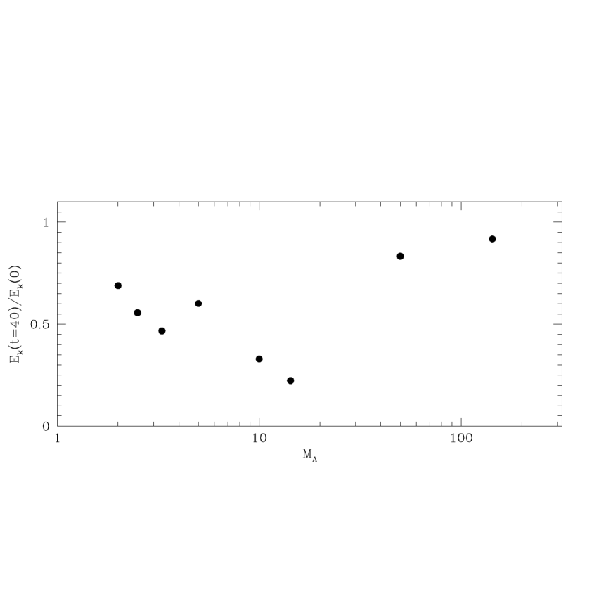
Figure 5.— The kinetic energy left at the end of simulations ($t=40$). It is normalized to the initial value. This provides a measure of kinetic energy dissipation.

Figure 6.— Time evolution of the ratio of the mean $B_{z}$ in the top region, ${L/2}<y<L$, over that in the bottom region, $0<y<{L/2}$. Curves are labeled with $M_{A}$.

Figure 7.— Maximum extent of non-zero $B_{z}$ in the $y$ direction during the simulations.

Figure 8.— Evolution of the $x$ average value of $B_{z}$ for the case with $M_{A}=14.3$.

Figure 9.— The mean velocity profile as a function of $y$ at $t=40$ for the stronger field cases. Curves are labeled with $M_{A}$.

Table 1Initial Parameters of Simulations.

$B_{0}$	$M_{A}(=U_{0}/c_{A})$	$\beta_{0}=p/p_{b}$	Uniform Field Evolution	Sheared Field Evolution
$0.007$	$142.9$	$2.4\times 10^{4}$	dissipative	dissipative
$0.02$	$50$	$3000$	dissipative	dissipative
$0.07$	$14.3$	$245$	disruptive	disruptive
$0.1$	$10$	$120$	disruptive	disruptive
$0.2$	$5$	$30$	disruptive	asymmetric
$0.3$	$3.3$	$13.3$	nonlinearly stable	asymmetric
$0.4$	$2.5$	$7.5$	nonlinearly stable	asymmetric
$0.5$	$2$	$4.8$	marginally stable	asymmetric

References

- (1) Biskamp, D. 1994, Physics Rept., 237, 179
- (2) Bodo, G., Rossi, P., Massaglia, S., Ferrari, A., Malagoli, A., & Rosner, R. 1998, A&A, 333, 1117
- (3) Chandrasekhar, S. 1961, “Hydrodynamic & Hydromagnetic Stability”, (New York: Oxford University Press)
- (4) Corcos, G. M. & Sherman, F. S. 1984, J. Fluid Mech., 139, 29
- (5) Dahlburg, R. B., Boncinelli, P. & Einaudi, G. 1997, Phys. Plasmas, 4, 1213
- (6) Dahlburg, R. B. & Karpen, J. T. 1995, JGR, 100, 23489
- (7) Ferrari, A., Trussoni, E. & Zaninetti, L. 1981, MNRAS, 196, 1051
- (8) Frank, A., Jones, T. W., Ryu, D., & Gaalaas, J. B. 1996, ApJ, 460, 777 (Paper I)
- (9) Galinsky, V. L. & Sonnerup, B. U. O., 1994, Geophys. Res. Lett., 21, 2247
- (10) Gregori, G., Miniati, F., Ryu, D. & Jones, T. W. 1999, preprint
- (11) Jones, T. W., Gaalaas, J. B., Ryu, D., & Frank, A. 1997, ApJ, 482, 230 (Paper II)
- (12) Jones, T. W., Ryu, D. & Frank, A. 1999, in Numerical Astrophysics, S, M, Miyama, K. Tomisaka & T. Hanawa, eds. (Dordrecht: Kluwer)
- (13) Jones, T. W., Ryu, D. & Tregillis, I. L. 1996, ApJ, 473, 365
- (14) Keller, K. A. & Lysak, R. L. 1999, preprint
- (15) Keppens, R., Tóth, G., Westermann, R. H. J., & Goedbloed, J. P. 1999, J. Plasma Physics (submitted) (astro-ph/9901166)
- (16) Kopp, R. A. 1992, in Coronal Streamers, Coronal Loops, and Coronal and Solar Wind Composition, Eur. Space Agency Spec. Publ., ESA SP-348, 53
- (17) Mac Low, M., Klessen, R. S., Burkert, A. & Smith, M. D. 1998, Phys Rev. Lett., 80, 2754
- (18) Malagoli A., Bodo G., & Rosner R. 1996, ApJ, 456, 708
- (19) Maslowe, S. A. 1985, in Hydrodynamic Instabilities and the Transition to Turbulence, ed. H. L. Swinney and J. P. Gollub (Berlin, Springer-Verlag), p 181
- (20) Miniati, F., Jones, T. W. & Ryu, D. 1999, ApJ, 517, 242
- (21) Miura, A. 1984, JGR, 89, 801
- (22) Miura, A. 1987, JGR, 92, 3195
- (23) Miura, A. & P. L. Pritchett 1982, JGR, 87, 743
- (24) Ouyed, R. & Pudritz, R. E. 1997, ApJ, 482, 712
- (25) Porter, D. H., & Woodward, P. R. 1994, ApJS, 93, 309
- (26) Ryu, D. & Jones, T. W. 1995, ApJ, 442, 228
- (27) Ryu, D., Jones, T. W., & Frank, A. 1995, ApJ, 452, 785
- (28) Ryu, D., Jones, T. W., & Frank, A. 1999, preprint
- (29) Russell, C. T. 1990, in Physics of Magnetic Flux Ropes, C.T. Russell, E. R. Priest & L. C. Lee, eds. (Washington, D.C.: American Geophysical Union)
- (30) Stone, J. M., Ostriker, E. C. & Gammie, C. F. 1998, ApJ, 508, L 99
- (31) Weiss, N. O. 1966, Proc. Roy. Soc. London, A, 293, 310
- (32) Wu, C. C. 1986, JGR, 91, 3042
- (33) Yi, Y., Walker, R. J., Ogino, T. & Brandt, J. C. 1996, JGR, 101, 27585