The Role of Mixing in Astrophysics

Abstract

The role of hydrodynamic mixing in astrophysics is reviewed, emphasizing connections with laser physics experiments and inertial confinement fusion (ICF). Computer technology now allows two dimensional (2D) simulations, with complex microphysics, of stellar hydrodynamics and evolutionary sequences, and holds the promise for 3D. Careful validation of astrophysical methods, by laboratory experiment, by critical comparison of numerical and analytical methods, and by observation are necessary for the development of simulation methods with reliable predictive capability. Recent and surprising results from isotopic patterns in presolar grains, 2D hydrodynamic simulations of stellar evolution, and laser tests and computer simulations of Richtmeyer-Meshkov and Rayleigh-Taylor instabilities will be discussed, and related to stellar evolution and supernovae.

1 Introduction

In astronomy, mixing is important in two widely different situations. First, there is the mixing of chemically discrete materials. Here we consider the interstellar medium, and sufficiently cold environments that solid particles (grains) may survive (Clayton (1982)). This area is exciting now due to direct experimental identification of presolar grains (see Anders & Zinner (1993); Huss, et al. (1994); Bernatowicz & Zinner (1997), and references therein).

The second situation involves the mixing of plasma which differs in its isotopic composition; this is vital to the evolution of stars, which produce isotopic and nuclear variation by thermonuclear burning (Clayton (1968); Arnett (1996)). Thermonuclear burning is analogous to chemical combustion in many ways, and may be as complex. Mixing becomes important in determining whether flame can spread to new fuel, or is choked by build up of ashes. Mixing, even in small degree, can provide indications of ashes which can be used to diagnose burning conditions.

2 Mixing

We sometimes forget that stars are really very large. Let us make a order of magnitude estimate of diffusion time scales in a dense stellar plasma. It is the nuclei, not the electrons which define the composition. The coulomb cross section for pulling ions past each other is of order $\sigma\approx 10^{-16}\rm\ cm^{2}$. For a number density $N\approx 10^{24}\rm\ cm^{-3}$, this implies a mean free path $\lambda=1/\sigma N\approx 10^{-8}\rm\ cm$. For a particle velocity $v_{d}\approx 10^{8}\rm\ cm/s$, this gives a diffusion time $\tau_{d}=(\Delta r)^{2}/\lambda v_{d}\approx(\Delta r)^{2}\rm\ s\ cm^{-2}$. For a linear dimension of stellar size, $\Delta r=10^{11}\rm\ cm$, $\tau_{d}=3\times 10^{14}\rm\ y$, or 3,000 Hubble times! While one may quibble about the exact numbers used, it is clear that pure diffusion is ineffective for mixing stars, except for extreme cases involving extremely long time scales and steep gradients.

Actually, we all know from common experience—such as stirring cream into coffee (tea)—that this discussion is incomplete. To diffusion must be added advection, or stirring. Stars may be stirred too. For example, rotation may induce currents, as may accretion, and perturbations from a binary companion. However, the prime mechanism for stirring that is used in stellar evolutionary calculations is thermally induced convection. The idea is that convective motions will stir the heterogeneous matter, reducing the typical length scale $\Delta r$ to a value small enough that diffusion can insure microscopic mixing. For our stellar example above, this would require a reduction in scale of $(\lambda/\Delta r)^{1/2}\approx 10^{-8}$. Convection is not perfectly efficient, so that the actual mixing time would still be finite. Given that such a limit exists, we must examine rapid evolutionary stages to see if microscopic mixing is a valid approximation. For presupernovae, the approximation is almost certainly not correct, so that these stars are not layered in uniform spherical shells as conventionally assumed, but heterogeneous in angle as well as radius.

3 What The Light Curves Tell Us

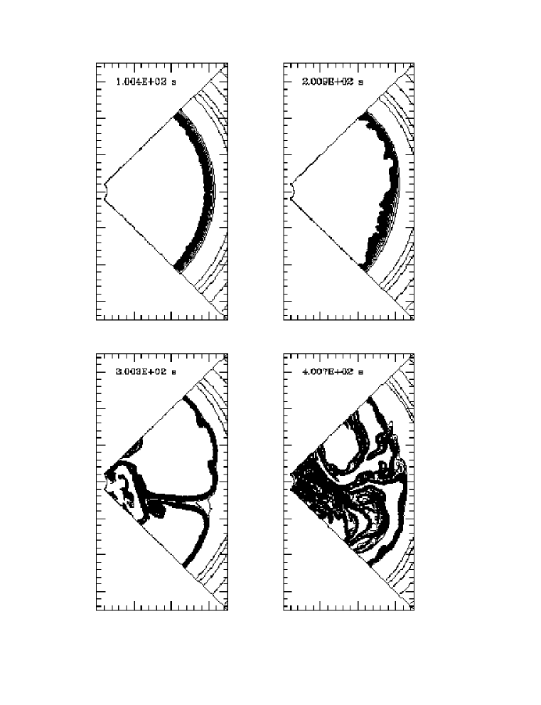
Figure 2: Snapshots of plumes of $\rm{}^{12}C$, after Bazan & Arnett (1998). Such effects are poorly represented by spherically symmetric simulations.

One of the most noticed aspects of SN1987A was the fact that the progenitor was not a red supergiant, as most stellar evolutionary calculations predicted, but had a smaller radius, $r\approx 3\times 10^{12}\ \rm cm$. The nature of the HR diagram for massive stars in the LMC was already an old problem (El Eid, et al. 1987, Maeder 1987, Renzini 1987, Truran & Weiss 1987). In retrospect, this expectation of a red supergiant was due to the implicit assumption that semiconvective mixing was instantaneous, and that the Schwarschild gradient was the one to use (this is more reasonable for lower mass stars, which evolve more slowly, see Chapter 7 in Arnett 1996). As luck would have it, my formulation of the stellar evolutionary equations gave the Ledoux criterion as the default, and the progenitor was a “blue” supergiant when the core collapsed (Arnett 1987). An example is shown in Figure 2, with the error box for the observed progenitor, Sk -69 202. This type of behavior is robust in the sense that, as long as the criterion is similar to the Ledoux one, LMC star models around 20 solar masses will loop back from the red giant branch when they do core carbon burning. The actual physical nature of this mixing process (presumably due to the double diffusion of ions and heat) does not seem well understood, at least in this context. The “blue” nature of the progenitor could be due to some other cause, of course, such as interaction or merger with a binary companion, but no such complex scenario is required for this position in the HR diagram.

After the euphoria of realizing that SN1987A actually was a close supernova, I happily simulated the early light curve by running shocks through stellar models of appropriate radius and mass. This worked fine for the first twenty days of data (Arnett 1987), but then the agreement degraded between the observed and computed light curves, as shown in Figure 1. Further, synthesis of the spectra was no longer successful at this epoch (Lucy 1987). This was followed by the Bochum event in the evolution of the spectra (Hanuschik & Dachs 1987), and later by the early emergence of x-rays (Donati, et al. 1987, Sunyaev, et al. 1987) and detection of $\gamma$-ray lines (Matz et al. 1987). Something more was happening than implied by the spherically symmetric models.

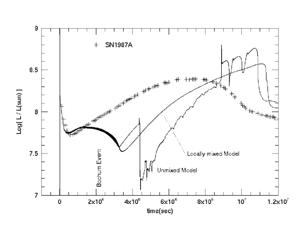
Figure 1: Observed and Simulated Light Curves for SN1987A.

While the powerful tools of radiation hydrodynamics were failing, a far simpler tool succeeded: after the first two weeks in which the effects of shock break-out were still felt, an analytic model (see Arnett 1996 and references therein) reproduced the observed light curve much more accurately. To obtain the analytic solution, it was necessary to assume that the opacity was relatively uniform and the radioactive Ni, while centrally concentrated, was distributed half-way to the surface! It seemed that some sort of mixing had occurred after the $\rm{}^{56}Ni$ was synthesized in the explosion.

Various amounts of arbitrary mixing were added to the simulations to obtain a match to the observed light curve (ABKW 1989). It is easy to assume mixing as an ad hoc process, but considerably more demanding to make a plausible simulation of how the mixing actually occurs. Figure 1 illustrates some options. The observational data for the UVOIR light curve are shown as crosses. The analytic model fits from about $t=10^{6}\ \rm sec$ onward (see Figure 13.8 in Arnett 1996). A one-dimensional numerical model without mixing is labeled “unmixed.” As the photosphere moves into the burned layers, wild variations in luminosity occur as the ionization state varies, and hence in the dominant opacity (which is due to Thomson scattering from free electrons). More careful treatment of spherical effects will smooth this only slightly (over a time $r/c\approx 3\times 10^{4}\ \rm seconds$). If neighboring zones which are convectively unstable ($\nabla\rho\times\nabla P<0$) are instantaneously mixed, the curve labeled “locally mixed model” is obtained. This maximal local mixing case is inadequate to explain the result. This implies that multidimensional effects—in particular, advection—are in operation. The mixing is not defined solely by local properties, but rather is deeply nonlinear. Subsequent data from much later stages supports this conclusion (Wooden 1997, McCray 1997).

4 Mixing by Advection and/or Diffusion

Stars are thermonuclear reactors, so that the change of abundances both drives the evolution and provides a diagnostic of that process. The rate of change in nuclear abundance $Y_{i}$ is usually assumed to be governed by the set of equations,

$$dY_{i}/dt=-Y_{i}Y_{j}R_{ij}-\cdots+Y_{k}Y_{l}R_{kl}+\cdots$$ (1)

in which all participating species (denote by indices i, j  k, l) are included. Only binary reactions are explicitly shown, for brevity. The nuclear reaction rates are denoted $R_{ij}$, with the indices ij running through the corresponding species. See Arnett (1996) for detail.

If we are not dealing with homogeneous matter, complications arise (Arnett 1997). First, gradients are not zero, so that we have variations in both space and time. The ordinary differential equations become partial differential equations. As seen from a fixed frame, with material flowing past, the operator $dY_{i}/dt$ becomes $\partial Y_{i}/\partial t+{\bf v\cdot\nabla}Y_{i}$, where ${\bf v}$ is the fluid velocity. The new second term is advection. This gives,

$$\partial Y_{i}/\partial t+{\bf v\cdot\nabla}Y_{i}=-Y_{i}Y_{j}R_{ij}-\cdots+Y_{k}Y_{l}R_{kl}+\cdots,$$ (2)

which couples the abundance distribution to the hydrodynamic flow. Energy release or absorption by nuclear burning further affect the flow. The system may now be heterogeneous.

Second, if gradients in composition (e.g., in $Y_{i}$) are present, then a new term is generated when we move to the fluid frame. The velocities of nuclei are split into a symmetric part around the center of momentum (characterized by a temperature $T$), and the fluid velocity $\bf v$. With a composition gradient, the flux of composition is nonzero, unlike the flux of momentum in the comoving frame. This gives rise to source terms due to diffusion (Landau & Lifshitz 1959), which in the continuity equation for species have the form $-{1\over\rho}{\bf\nabla\cdot F_{i}}$, where the composition flux is ${\bf F_{i}}=\rho Y_{i}{\bf v}$. Thus,

$$\partial Y_{i}/\partial t+{\bf v\cdot\nabla}Y_{i}=-Y_{i}Y_{j}R_{ij}-\cdots+Y_{k}Y_{l}R_{kl}+\cdots-{1\over\rho}{\bf\nabla\cdot F_{i}}.$$ (3)

If the composition gradients are small, we approximate ${\bf F_{i}}\approx-\rho D{\bf\nabla}Y_{i}$; this is the usual diffusion flux for composition, with the diffusion coefficient $D\approx\lambda v_{d}/3$, where $\lambda$ is the diffusion mean free path and $v_{d}$ the mean velocity of diffusing particles relative to the fluid frame. Notice that the diffusion and advection terms may act on strongly differing length scales in this equation.

We may recover the original simplicity of Eq. 1 if either (1) the region of interest (the computational “zone”) is really homogeneous, or (2) it is very well mixed (large diffusion coefficient D). In the limit of many mean free paths taken, diffusion approximates a random walk process. Because of the benign numerical properties of the diffusion operator, stellar evolutionists have often used some variety of diffusion to model convective mixing, assuming that $\lambda$ is approximately a mixing length $\ell$, and many paths were taken. Note that this involves the singular idea that scales of order $\lambda\approx 10^{-8}\rm cm$ are equivalent to those of order $\ell\approx 10^{+8}\rm cm$ or more. Ignoring the advection term, this gives,

$$\partial Y_{i}/\partial t\approx-Y_{i}Y_{j}R_{ij}-\cdots+Y_{k}Y_{l}R_{kl}+\cdots-{1\over\rho}{\bf\nabla\cdot F_{i}},$$ (4)

which is an approximation to Eq. 3, and is commonly used in stellar evolutionary codes (e.g., Woosley & Weaver 1995). It ignores advection, which is the dominant mode of macroscopic mixing.

5 Applications to Stellar Hydrodynamics

In discussion of stellar evolution, one encounters the topics of rotation, convection, pulsation, mass loss, micro-turbulence, sound waves, shocks, and instabilities—to name a few—which are all just hydrodynamics. However, direct simulation of stellar hydrodynamics is limited by causality. In analogy to light cones in relativity, in hydrodynamics one may define space-time regions in which communication can occur by the motion of sound waves. To correctly simulate a wave traveling through a grid, the size of the time step must be small enough so that sound waves cannot “jump” zones. Thus the simulation is restricted to short time steps—an awkward problem if stellar evolution is desired. While simulations of the solar convection zone are feasible, the simulation time would be of order hours instead of the billions of years required for hydrogen burning. For the latter, a stellar evolution code is used, which damps out the hydrodynamic motion, obviating the need for the time step restriction. Any presumed hydrodynamic motion is then replaced by an algorithm (such as adiabatic structure and complete mixing in formally convective regions). Thus, stellar evolution deals with the long, slow phenomena, and stellar hydrodynamics has dealt with the short term.

However, the stages of evolution prior to a supernova explosion are fast and eventful. Here direct simulation is feasible (Bazan & Arnett (1998)). A key region for nucleosynthesis is the oxygen burning shell in a presupernova star. Besides producing nuclei from Si through Fe prior to and during the explosive event, it is the site at which the radioactive $\rm{}^{56}Ni$ is made and is mixed. The conventional picture of this region relies upon the notion of thermal balance between nuclear heating and neutrino cooling in the context of complete microscopic mixing by convective motions.

This is usually treated by the mixing length scenario for convection, which assumes statistical (well developed) turbulence, random walk of convective blobs approximated by diffusion, subsonic motions, and almost adiabatic flow. These approximations are further constrained by a simplistic treatment of the boundaries of the convective region.

The time scales for the oxygen burning shell are unusual. The evolutionary time is $\tau_{evol}\approx 4\times 10^{3}\rm\ s$. The convective “turnover” time is $\tau_{conv}\approx\Delta r/v_{conv}\approx\tau_{evol}/10$, while the sound travel time across the convective region is $\tau_{sound}\approx\Delta r/v_{sound}\approx\tau_{conv}/100$. The burning time is $\tau_{burn}=E/\varepsilon\leq\tau_{conv}$. Obviously the approximations of subsonic flow, well developed turbulence, complete microscopic mixing, and almost adiabatic flow are suspect.

These time scales are rapid enough to make the oxygen shell a feasible target for direct numerical simulations, and an extensive discussion has appeared (Bazan & Arnett (1998), and Asida & Arnett, in preparation). The two dimensional simulations show qualitative differences from the previous one dimensional ones. The oxygen shell is not well mixed, but heterogeneous in coordinates $\theta$ and $\phi$ as well as $r$. The burning is episodic, localized in time and space, occurring in flashes rather than as a steady flame. The burning is strongly coupled to hydrodynamic motion of individual blobs, but the blobs are more loosely coupled to each other.

Acoustic and kinetic luminosity are not negligible, contrary to the assumptions of mixing length theory. The flow is only mildly subsonic, with mach numbers of tens of percent. This gives nonspherical perturbations in density and temperature of several percent, especially at the boundaries of the convective region.

At the edges of convective regions, the convective motions couple to gravity waves, giving a slow mixing beyond the formally unstable region. The convective regions are not so well separated as in the one dimensional simulations; “rogue blobs” cross formally stable regions. A carbon rich blob became entrained in the oxygen convective shell, and underwent a violent flash, briefly out-shining the oxygen shell itself by a factor of 100. Significant variations in neutron excess occur throughout the oxygen shell. Because of the localized and episodic burning, the typical burning conditions are systematically hotter than in one dimensional simulations, sufficiently so that details of the nucleosynthesis yields will be affected.

The two dimensional simulations are computationally demanding. Our radial zoning is comparable to that used in one dimensional simulations, to which we add several hundred angular zones, giving a computational demand several hundred times higher. This has limited us to about a quarter of the final oxygen shell burning in a SN1987A progenitor model. Given the dramatic differences from one dimensional simulations, it is important to pursue the evolutionary effects to see exactly how nucleosynthesis yields, presupernova structures, collapsing core masses, entropies, and neutron excesses will be changed. It may be that hydrostatic and thermal equilibrium on average, and the temperature sensitivity of the different burning stages, taken together, tend to give a rough layering in composition, even if the details of how this happens are quite different.

6 Toward a Predictive Theory: Tests
with The NOVA Laser

Ultimately simulations must be well resolved in three spatial dimensions. One of the great assets of computers is their ability to represent complex geometries. If we can implement realistic representations of the essential physics, then simulations should become tools to predict—not “postdict”—phenomena. An essential step toward that goal is the testing of computer simulations against reality in the form of experiment (Remington, Weber, Marinak, et al. (1995)). This is a venue in which we can alter conditions (unlike astronomical phenomena), and thereby understand the reasons for particular results. Experiments are intrinsically three dimensional, with two dimensional symmetry available with some effort, so that they provide a convenient way to assess the effects of dimensionality.

For Rayleigh-Taylor instabilities, the NOVA experiments not only sample temperatures similar to those in the helium layer of a supernova, but hydrodynamically scale to the supernova as well (Kane, et al. (1997)). In the same sense that aerodynamic wind tunnels have been used in aircraft design, these high energy density laser experiments allow us to precisely reproduce a scaled version of part of a supernova.

The NOVA laser is physically imposing. The building is larger in area than an American football field; the lasers concentrate their beams on a target about the size a BB (or a small ball bearing). This enormous change in scale brings home just how high these energy densities are. Preliminary results show that the astrophysics code (PROMETHEUS) and the standard inertial confinement fusion code (CALE) both give qualitative agreement with the experiment. For example, the velocities of the spikes and bubbles are both in agreement with experiment, and analytic theory which is applicable in this experimental configuration (Kane, et al. (1997)). The two codes give similar, but not identical results. These differences will require new, more precise experiments to determine which is most nearly correct.

References

- Anders & Zinner (1993) Anders, E., & Zinner, E., 1993, Meteoritics 28, 490
- Arnett (1996) Arnett, D. 1996, Supernovae and Nucleosynthesis, Princeton: Princeton University Press
- Bazan & Arnett (1998) Bazan, G., & Arnett, D., 1998, ApJ 496, 316
- Bernatowicz & Zinner (1997) Bernatowicz, T. J., & Zinner, E., 1997, Astrophysical Implications of the Laboratory Study of Presolar Materials, AIP Conference Proceedings 402, Woodbury, NY: American Institute of Physics
- Clayton (1968) Clayton, D. D., 1968, Principles of Stellar Evolution and Nucleosynthesis, New York: McGraw-Hill
- Clayton (1982) Clayton, D. D., 1982, QJRAS, 23, 174
- Huss, et al. (1994) Huss, G. R., Fahey, A. J., Gallino, R., & Wasserburg, G. J., 1994, ApJ 430, 81
- Kane, et al. (1997) Kane, J., Arnett, D., Remington, B., Glendinning, S. G., Castor, J., Wallace, R., Rubenchik, A., Fryxell, B. A., 1997, ApJ 478, 75
- Remington, Weber, Marinak, et al. (1995) Remington, B. A., Weber, S. V., Marinak, M. M., et al., Phys. Plasmas 2, 241, 1995.