Evolution of Multi-mass Globular Clusters in Galactic Tidal Field with the Effects of Velocity Anisotropy

Abstract

We study the evolution of globular clusters with mass spectra under the influence of the steady Galactic tidal field, including the effects of velocity anisotropy. Similar to single-mass models, velocity anisotropy develops as the cluster evolves, but the degree of anisotropy is much smaller than isolated clusters. Except for very early epochs of the cluster evolution, nearly all mass components become tangentially anisotropic at the outer parts. We have compared our results with multi-mass, King-Michie models. The isotropic King model better fits to the Fokker-Planck results because of tangential anisotropy. However, it is almost impossible to fit the computed density profiles to the multi-mass King models for all mass components. Thus if one attempts to derive global mass function based on the observed mass function in limited radial range using multi-mass King models, one may get somewhat erratic results, especially for low mass stars. We have examined how the mass function changes in time. Specifically, we find that the power-law index of the mass function decreases monotonically with the total mass of the cluster. This appears to be consistent with the behaviour of the observed slopes of mass functions for a limited number of clusters, although it is premature to compare quantitatively because there are other mechanisms in contributing the evaporation of stars from the clusters. The projected velocity profiles for anisotropic models with the apocenter criterion for evaporation show significant flattening toward the tidal radius compared to isotropic model or anisotropic model with the energy criterion. Such a behaviour of velocity profile appears to be consistent with the observed profiles of collapsed cluster M15.

1 INTRODUCTION

The study of evolution of globular clusters has a long history. It would be most desirable to use direct $N$-body calculations in order to follow the evolution of realistic globular clusters realistically, but we do not have enough computing power to do that for $N$ comparable to the number of stars in real globular clusters at this moment. Therefore we have to rely on approximate techniques to understand the dynamics of star clusters. The Fokker-Planck equation has been widely used for the study of globular clusters, but it requires many simplifying assumptions. The assumption of velocity isotropy is usually employed because it allows fast and accurate integration of the Fokker-Planck equation (Cohn 1980). However, high degree of velocity anisotropy is known to be generated by two-body relaxation in the outer parts of isolated clusters (e.g., Spitzer 1987). The observational properties of the clusters depend on the degree of anisotropy and correct treatment of anisotropy becomes an important issue. The development of velocity anisotropy was investigated in some recent works which used various numerical methods: e.g., direct $N$-body calculations by Giersz & Heggie (1994), gaseous model calculations by Louis & Spurzem (1991) and Spurzem (1996), and Fokker-Planck calculations by Cohn (1979), Drukier et al. (1999) and Takahashi (1995, 1996, 1997). Most of these calculations confirmed the earlier expectations of generation of radial anisotropy in the outer parts of the clusters, although detailed behaviour depends somewhat on the numerical methods.

Actual clusters are embedded in the Galactic tidal field which should impose a finite boundary to the cluster. The introduction of tidal boundaries should have significant effects on the velocity anisotropy. Recently Takahashi, Lee & Inagaki (1997; abbreviated as TLI hereafter) performed anisotropic Fokker-Planck simulations for single mass clusters and demonstrated that radial anisotropy grows up to the time of core collapse, but the degree of anisotropy begins to decrease to smaller values as the cluster expands and loses significant amount of mass. They showed that there is even tangential anisotropy very close to the tidal boundary in the late phase of the cluster’s evolution. The density profiles of the clusters can be reasonably fitted by isotropic King models for most of the time except for the brief phase around the core collapse, when the degree of radial anisotropy nearly reaches its maximum.

The behaviour of the anisotropy for isolated clusters with mass spectra has some interesting features. Takahashi (1997) showed that the degree of anisotropy for different mass components behaves differently. There is always radial anisotropy for low mass components, but tangential anisotropy can develop for high mass components at early evolutionary stages when the temperature of heavy stars decreases rapidly toward the equipartition. During this ‘cooling’ phase, the radial velocity dispersion decreases more rapidly than the tangential one. This leads to the development of tangential anisotropy among high mass stars.

As in the case of single mass models, extension of these studies into tidally limited clusters should provide useful insight on the evolution of realistic clusters. Based on the experience of single mass models, one obviously expects that the velocity anisotropy will be greatly affected by the presence of the tidal field. Some of the essential points have been clarified by the analyses of $N$-body results (Vesperini & Heggie 1997), but one should remember that the $N$-body calculations are done for small $N$ cases. Many of the behaviour of self-gravitating systems does not allow simple scaling (e.g., Portegies Zwart et al. 1998, Takahashi & Portegies Zwart 1998). We make detailed calculations for the evolution of globular clusters with these effects in order to make quantitative assessments for the long term evolution of star clusters with the tidal cut-off and mass spectrum.

The study of the evolution of tidally limited clusters has important areas of application. The mass function of globular clusters is difficult to obtain because of large dynamic range in brightness of individual stars as well as large variation of stellar densities. It is very difficult to determine the global mass function observationally, but there have been several studies to determine the global mass function based on locally measured mass functions in limited areas of globular clusters (Richer et al. 1990, 1991 and references therein). It is absolute necessity to obtain the global mass function if one wants to study factors determining the mass function of clusters. The conversion of the local mass function to the global one is not a trivial task. The general practice employed widely is to fit the observation to multi-mass King models (e.g., Meylan 1988) or to assume that the mass function in low mass stars in the outer parts are close to the global one (Richer et al. 1991). However, there is no guarantee that these processes give a right answer. The detailed studies of evolving clusters with the tidal boundary can provide an important check of the above mentioned practices.

The mass function changes with time because the rate of escape of stars depends on the mass of the star. The high mass stars tend to spiral into the central parts by dynamical friction, and consequently low mass stars are preferentially removed from the tidally limited clusters. The slope of mass function thus becomes less steep as the cluster loses mass. Even if one gets the global mass function through careful observations and correct conversion process, the present day mass function (PDMF) may be significantly different from the initial mass function (IMF). The detailed studies of evolving star clusters could provide an important framework of estimating the relation between PDMF and IMF.

In the present paper, we make detailed studies of the the evolution of tidally limited multi-mass clusters including the effects of velocity anisotropy. We pay special attention to the behaviour of mass function during the course of dynamical evolution. We examine the adequacy of the process of converting the local mass function to the global mass function using multi-mass King model fitting. We then analyze how the mass function changes with time and location.

This paper is organized as follows. In § 2, we describe our models for the evolution of globular clusters. In § 3, we introduce the idea of half-mass concentration and discuss its relation to the development of anisotropy and to mass loss rates. In § 4 we describe initial conditions of multi-mass models. In § 5 we present the results of the model calculations. The relationship between local and global mass function and the temporal evolution of mass function are examined in § 6. We discuss the velocity dispersion profiles in §  7. The final section summarizes basic results.

2 Fokker-Planck Models

We use the anisotropic Fokker-Planck code developed by Takahashi (1995). It is based on the direct integration method of the Fokker-Planck equation in $(E,J)$ space (Cohn 1979), where $E=v^{2}/2+\phi(r)$ is the energy of a star per unit mass and $J=rv_{t}$ is the angular momentum per unit mass. The extension to multi-mass clusters is described in Takahashi (1997) and the treatment of tidal boundary can be found from TLI. TLI used two different criteria for the escape of a star from the cluster: apocenter criterion and energy criterion. The apocenter criterion assumes that a star escapes if the apocenter distance of a star with $(E,J)$ becomes greater than tidal radius $r_{t}$. This criterion preferentially removes the stars with low $J$ and thus suppresses the development of radial anisotropy. The $energy$ criterion assumes that a star escapes if $E>E_{t}$ where $E_{t}=\phi(r_{t})$. The radial anisotropy is also suppressed in this criterion and tangential anisotropy can develop (see TLI). The general behaviour of the cluster evolution is not much dependent on the choice of escape criteria for the models of TLI, but details of the clusters vary with the treatment of stellar evaporation. Takahashi & Portegies Zwart (1998) have shown that the apocenter criterion gives better results when compared with realistic $N$-body calculations. In the present study, we examine the results of our calculations with both of the criteria, but more emphasis is given to the calculations with the apocenter criterion.

Hereafter, we denote anisotropic models with the apocenter criterion as Aa models and anisotropic models with the energy criterion as Ae models. The capital A stands for anisotropic models, and the lower cases a and e stand for apocenter and energy criteria, respectively. Similarly isotropic models are denoted as Ie models, but Ia models do not exist.

3 Half-Mass Concentration, Velocity Anisotropy, and the Mass Loss Rate

Before going into descriptions of the results of multi-mass models, we examine the effects of the degree of the concentration of a cluster on the development of velocity anisotropy and on the cluster mass loss rate. We use single-mass models in this section because these models are simple, but the conclusions of this section are also true for multi-mass models, as we show later.

TLI used the initial model of a single-mass Plummer model with the cutoff radius of 32 in Plummer model units. The results of their simulations show that the Aa and Ae models lose mass faster than the Ie model (see Fig. 2a of TLI, though the Ae model is not shown in it). The evaporation time of the Ie model is about 12% longer than that of the Aa model, and the latter is about 10% longer than that of the Ae model. The biggest difference in the mass loss rate between the anisotropic models and the isotropic model appears in the pre-collapse and the early post-collapse phases. The mass loss rates of the different models are similar in the late post-collapse phase.

In § 5 we show the results of simulations which start with multi-mass King models. As shown in Fig. 4, the Ie model and the Ae model are very similar in the evolution of the total mass. The Aa model loses mass slower than the Ie model. This trend is opposite to that seen in the simulations of TLI. While Fig. 4 shows the results for a $W_{0}=3$ King model, the same trend is seen for King models with other $W_{0}$. Why does the opposite trend appear? The change from the single-mass model to the multi-mass model is not the reason of the change of the trend. Rather, it is found that the trend changes with the concentration of a cluster to the tidal cutoff radius.

First we discuss what parameter is useful in measuring the degree of the concentration of a cluster. For King models, the concentration is usually measured in terms of the concentration parameter $c\equiv\log_{10}(r_{\rm t}/r_{0})$, where $r_{0}$ is the King core radius (King 1966). The parameter $c$ is useful in measuring the concentration of the core. However, when discussing the variation of the total mass, $c$ is not always an appropriate parameter, because the fraction of the core mass is very small in large $c$ clusters. It may be more appropriate to use the half-mass radius $r_{\rm h}$ instead of the core radius $r_{0}$. Thus we define half-mass concentration

$$c_{\rm h}\equiv r_{\rm t}/r_{\rm h},$$ (1)

(note the logarithm is not taken here).

King models form a one-parameter family parameterized by the concentration $c$ or equivalently by the dimensionless central potential depth $W_{0}$; $c$ monotonically increases with $W_{0}$ (King 1966). On the other hand, $c_{\rm h}$ does vary monotonically with $W_{0}$. The relation among $W_{0}$, $c$, and $c_{\rm h}$ is given in Fig. 1 for $1\leq W_{0}\leq 14$. In contrast to that the core concentration $c$ varies by nearly three orders of magnitude, the variation of the half-mass concentration $c_{\rm h}$ is within a factor of three for this range of $W_{0}$. The half-mass concentration $c_{\rm h}$ increases with $W_{0}$ for $W_{0}=1$ to 8, then it decreases until $W_{0}$ reaches and increases again. For the range of $1\leq W_{0}\leq 14$, $c_{\rm h}$ reaches the maximum of about 10 at $W_{0}\simeq 8$. The initial model of TLI has $c_{\rm h}=25$, therefore it is far more concentrated than any King models in terms of the half-mass concentration.

Figure 1: The behaviour of $c_{h}$, $c$, and $\xi_{AS}$ for King models against $W_{0}$. Note that $c_{h}$ has a maximum, and $\xi_{AS}$ has a broad minimum near $W_{0}\simeq 8$.

In order to investigate the effects of the half-mass concentration on the cluster evolution, we carry out simulations which start with single-mass Plummer models with different cutoff radii which correspond to $c_{\rm h}=$10, 20, and 30. In these simulations the number of particle is set to $10^{4}$, which is specified to include the effects of three-body binary heating. Fig. 2 shows the evolution of the total mass for the Ae and Ie models. For the large $c_{\rm h}$ initial models, the Ae model loses mass much faster than the Ie model at the early evolutionary phase as in TLI’s simulations. (The core collapse occurs at $t=$16–18$~{}t_{\rm rh,0}$ in all the models.) As $c_{\rm h}$ decreases, the difference between the Ae and Ie models decreases and finally almost diminishes for $c_{\rm h}=10$. Fig. 3 shows the evolution of the anisotropy $\beta$ at the 90%-mass radius. The anisotropy parameter $\beta$ is defined as follows:

$$\beta\equiv 1-{\sigma_{t}^{2}\over\sigma_{r}^{2}},$$ (2)

where $\sigma_{t}$ and $\sigma_{r}$ are one-dimensional tangential and radial velocity dispersions, respectively. The development of the radial anisotropy during the pre-collapse phase becomes strongly suppressed as $c_{\rm h}$ decreases. This is simply because radial-orbit stars can easily escape from a small tidal radius cluster. As TLI discussed, the emergence of a large number of radial-orbit stars is the reason for faster mass loss in the anisotropic models. For low $c_{\rm h}$ clusters, since there is almost no room for the radial anisotropy to develop, the Ae model and the Ie model do not differ very much in the evolution of the total mass. Since King models have such low $c_{\rm h}$ ($c_{\rm h}<10$), the difference among the three models shown in Fig. 4 can be understood from this viewpoint. The mass loss of the Aa model should be always slower than that of the Ae model because of the apocenter criterion (see TLI).

Note that we have assumed that the initial tidal radius is equal to the limiting radius of King models. This is a conventional way for setting up initial conditions of simulations, but not the only one; these two radii can be different.

Figure 2: The evolution of mass as a function of time for Ae models (dotted lines) and Ie models (dashed lines). The initial models are single-mass Plummer models with three different tidal cutoff radii: $c_{\rm h}\equiv r_{\rm t}/r_{\rm h}=$10, 20, 30, from left to right. As $c_{\rm h}$ decreases the mass loss becomes faster and the difference between the Ae model and the Ie model becomes smaller. The core collapse occurs at $t=$16–18$t_{\rm rh,0}$ in all the models.

Finally in this section, we comment on the relation between the mass loss rate and the half-mass concentration for King models. Johnstone (1993, figure 2) and Gnedin & Ostriker (1997, figure 6) found that for King models the mass loss rate per half-mass relaxation time (exactly speaking, the inverse of the evaporation time in units of the initial half-mass relaxation time in Gnedin & Ostriker) has a minimum around $c=$1.5–2. Johnstone (1993) calculated the evaporation rate for King models using the local Fokker-Planck equation, and Gnedin & Ostriker (1997) performed isotropic orbit-averaged Fokker-Planck simulations with the initial conditions of King models. Their findings are qualitatively consistent with a simple estimation of the mass loss rate based on only the half-mass concentration $c_{\rm h}$. Naively one may think that the mass loss rate decreases as $c_{\rm h}$ increases. In fact $c_{\rm h}$ has the maximum at $W_{0}\simeq 8$ ($c\simeq 1.8$), where Johnstone (1993) and Gnedin & Ostriker (1997) found the minimum evaporation rate. In addition Johnstone (1993) found a local maximum of the mass loss rate at $c\simeq 2.6$. This may correspond to the fact that $c_{\rm h}$ has a local minimum at $c\simeq 2.7$ ($W_{0}\simeq 12$) as shown in Fig. 1. As an additional reference, we show the mass loss rate per half-mass relaxation time $\xi_{\rm AS}$ calculated from the modified Ambartsumian-Spitzer formula (Spitzer 1987, p.57; see also TLI) for King models in Fig. 1. This estimation is even quantitatively not very different from the result of more detailed calculations for $W_{0}\leq 8$ by Johnstone (1993).

Figure 3: The evolution of the anisotropy $\beta$ at the 90%-mass radius for the Ae models plotted in Fig. 2. The initial development of the radial anisotropy becomes strongly suppressed as $c_{\rm h}$ decreases from 30 to 10.

4 Multi-Mass Models

There are growing evidences that the mass function in clusters as well as in the field is not a simple power-law, but should be approximated as composite power-laws (e.g., Kroupa, Tout & Gilmore 1993). However, we use simple power-laws in the present study of general evolution of clusters, for simplicity. The adoption of multiple composite power-laws is trivial task, but requires specification of more model parameters. The assumed initial mass function (IMF) has the following form:

$$N(m)dm=Cm^{-\alpha}dm,\qquad m_{\rm min}\leq m\leq m_{\rm max},$$ (3)

where $C$ and $\alpha$ are constants. As in Takahashi (1997), we use the discrete mass components. The $i$-th mass bin for equal $\Delta\log m$ interval can be obtained by

$$m_{i}=m_{\rm min}\left({m_{\rm max}\over m_{\rm min}}\right)^{(i-{1\over 2})/K},\quad(i=1,2,...,K),$$ (4)

where $K$ is the number of components. The parameters determining the mass function are $\alpha$ and $\mu(\equiv{m_{\rm max}/m_{\rm min}})$. We use a few values of $\alpha$ and $\mu$ for our model calculations.

The issue of the effects of stellar evolution naturally comes out for multi-mass models if one extends the mass function to high mass stars. Obviously the stellar evolution should have been the most important process in determining the early phase of the dynamical evolution of globular clusters. However, we will ignore the stellar evolution in this paper because it adds one more complexity to the models.

Without stellar evolution, the clusters usually undergo core-collapse before losing significant amount of stars unless the initial cluster has very low central concentration, because the time scale for the core collapse is generally much shorter than the evaporation time. Note that the core collapse time is of order of $10t_{\rm rh,0}$ while the evaporation time is typically of order of $40t_{\rm rh,0}$, where $t_{\rm rh,0}$ is the initial half-mass relaxation time for single mass models. The core collapse is very much accelerated for multi-mass clusters, and the discrepancy between the evaporation time and the core collapse time could become even larger. Therefore one needs to supply the mechanism that allows the evolution of cluster beyond the core collapse. We assumed that the heating is provided by binaries formed by three-body processes because it is easiest to implement in the framework of Fokker-Planck method. The evolution of parameters for the central parts such as density and velocity dispersion should depend on the detailed mechanism for driving the post core-collapse evolution, but most of the global properties do not sensitively depend on the heating mechanism. For our purposes, three-body binary heating is sufficiently simple and easy to be used as heating mechanism. The heating formula for multi-mass clusters is taken from Lee, Fahlman & Richer (1991).

5 Results of Multi-Mass Model Calculations

5.1 Initial Model Parameters

We have used various initial models. The characteristics of the initial models are summarized in Table 1. In all models, we have assumed that the shape of density profiles of different mass components are the same with the different amplitudes dictated by the assumed mass functions. The velocity dispersions are assumed to be the same for all components. are assumed to have the same density and velocity profiles.

The behaviour of the cluster up to the core collapse does not depend on the initial total mass or size of the cluster. But the amount of binary heating depends on the number of stars in the cluster. We have assumed that the mass of the cluster is $6\times 10^{4}~{}{\rm\,M_{\odot}}$ for the model $R$, and we have fixed the total number of stars at $5\times 10^{4}$ for other models. But this number only controls the central density during the postcollapse phase. Most of our results does not really depend on the mass of the cluster, except for the surface density profiles. If we used higher initial mass, the core radii at a given epoch (measured by the $M/M_{0}$) would be smaller. The minimum mass $m_{min}$ of the mass function was assumed to be 0.1 ${\rm\,M_{\odot}}$ in all models.

Throughout this paper, we use $r$ to represent the distance from the center of the cluster, and $R$ to represent the projected distance.

5.2 A Reference Model

We first describe the general behaviour of Reference Model (Model R) whose initial parameters are given in Table 1. This set of parameters is used by Heggie et al. (1998) to compare the outcomes of various computational methods. We will consider this initial condition as a reference model. The number of mass component was 8.

Table 1: Initial Parameters for Multi-Mass Models

Model	Profile	$\alpha$	$\mu$	Comments
R	King, $W_{0}=3$	2.35	15	reference
K1	King, $W_{0}=3$	2.35	7	low $\mu$
K2	King, $W_{0}=8$	2.35	15	high $W_{0}$ ($c_{\rm h}$)
P1	Plummer, $c_{\rm h}=20$	2.35	15	high $c_{\rm h}$

5.2.1 Global behaviour

The evolution of the total mass is shown in Fig. 4 with different criteria for ejection of stars. Unlike single component models, the mass loss rate is not a constant, but increases with time. The increase of ${\dot{M}}$ is due to the fact that the mass function becomes flatter as the cluster loses mass. (The mass loss rate becomes larger for clusters with flatter mass function.) As discussed in §3, the apocenter criterion ($Aa$) gives longer lifetime than the energy criterion ($Ae$), but it is not a significant effect. For comparison, we have also shown the mass evolution for the isotropic model ($Ie$) with the same initial conditions. The time of maximum collapse is shown as dots in this figure.

Figure 4: The evolution of mass of the model $R$ of three different assumptions ($Aa$, $Ae$, and $Ie$). The mass loss rate is nearly a constant for single component models, but increases with time in our multi-mass models. This is due to the fact that the mass function becomes flatter as the cluster loses mass. The flatter mass function means higher mass loss rate.

5.2.2 Degree of anisotropy

The behaviours of the degree of velocity anisotropy $\beta$ for the apocenter criterion are shown in Figure 5. The upper, middle and lower panels show $\beta(r)$ at the time $M/M_{0}$=0.7, 0.5 and 0.2, respectively. The same figure as Fig. 5 for the energy criterion is shown in Fig. 6.

Figure 5: The dependence of $\beta$ on $r$ at three different epochs: $M/M_{0}$=0.7, 0.5 and 0.2 for $R$ models with the apocenter condition. The core-collapse occurs when $M/M_{0}\approx$ 0.70. Note that the low mass components show more tangential anisotropy than high mass stars. This is opposite to the isolated cluster models.

Figure 6: The dependence of $\beta$ on $r$ at three different epochs: $M/M_{0}$=0.7, 0.5 and 0.2 for $R$ models with energy condition. Note that the core-collapse occurs when $M/M_{0}\approx 0.57$. The velocity distribution is forced to become isotropic at tidal boundary in the energy condition.

Note that the sign of $\beta$ can be both positive (radial anisotropy) and negative (tangential anisotropy). If a cluster is isolated, strong radial anisotropy develops in the halo for all components, as shown by Takahashi (1997). However the present model cluster is in a rather strong tidal field: the initial King model with $W_{0}=3$ has $c_{\rm h}=3.7$. Therefore, from the discussion in § 3, we may expect that the development of such radial anisotropy is strongly suppressed in the present case. From the profiles shown in Fig. 5 (Aa model), in fact, only weak radial anisotropy is seen for the high mass components at intermediate radii. The low mass components tend to have tangential anisotropy at all radii. A similar trend is seen in Fig. 6 (Ae model). This is in sharp contrast with isolated clusters where strong radial anisotropy develops among low mass components (Takahashi 1997). In the top panel of Fig. 6, the high mass components also have tangential anisotropy. This is due to the initial cooling of the high mass components (Takahashi 1997). The velocity distribution becomes mostly tangential near the tidal boundary regardless of the mass. The tangential anisotropy was also noted by Oh & Lin (1992), and Kim & Oh (1999) from their hybrid calculation of N-body and Fokker-Planck.

The behaviour of $\beta(r)$ becomes different for apocenter and energy criteria in the outer parts, because the energy criterion forces $\beta$ at tidal boundary to become zero (i.e., isotropic).

5.2.3 Density profiles

The profiles of surface densities for different mass components are shown in Fig. 7 for a model with the apocenter condition at the epochs of $M/M_{0}=0.7$, 0.5 and 0.2. Fig. 8 shows the density profiles for a model with the energy condition. The density profiles at $M/M_{0}$=0.5 and 0.2 are similar for the apocenter condition and the energy condition. The big difference at $M/M_{0}$=0.7 is purely due to the fact that the core-collapse occurs when $M/M_{0}\approx$ 0.7 for the Aa model while it occurs somewhat later for the Ae model. Therefore, the difference in the degree of anisotropy at outer radii does not play important role in determining the density distribution.

Figure 7: Surface density distribution of individual mass components at three epochs for the $R$ model with apocenter criterion ($Aa$).

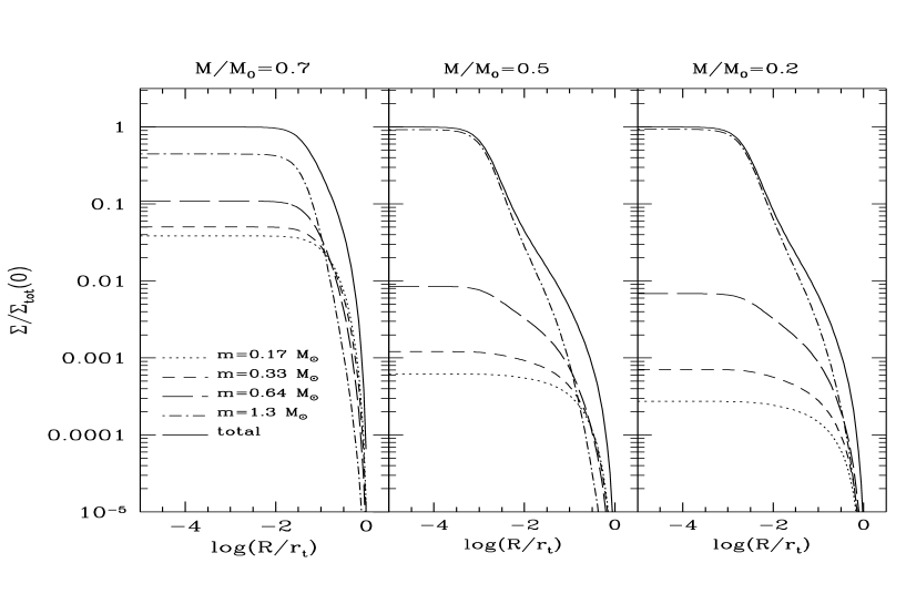
Figure 8: Surface density distribution of individual mass components at three epochs for the $R$ model with energy criterion ($Ae$).

The profiles at $M/M_{0}$=0.5 and 0.8 are compared with the isotropic model in Fig. 9. The radial profiles of the total density of isotropic and anisotropic models have very little difference, but the detailed distribution of individual mass components could be significantly different for these two models. From these comparisons, we expect that there will be some difference in the behaviour of the mass function in the lower mass parts at late phase of the evolution.

Figure 9: Comparison of density profiles of isotropic ($Ie$: thin lines) and anisotropic ($Aa$: thick lines) Fokker-Planck results at $M/M_{0}$=0.5 and 0.2.

In Fig. 10, we tried to compare the surface density profiles of the $R/Aa$ model at $M/M_{0}$=0.5 with the best-fitting multi-mass King models having the same mass function. Multi-mass King models have the following distribution function (e.g., Binney & Tremaine 1987):

$$f_{i}(E)=C_{i}\left[\exp(-E/\sigma_{i}^{2})-\exp(-E_{\rm t}/\sigma_{i}^{2})\right],\quad(i=1,2,...,K),$$ (5)

where $\sigma_{i}$ satisfies the relation $m_{i}\sigma_{i}^{2}=m_{j}\sigma_{j}^{2}$ for all $i$ and $j$. The constants $C_{i}$ should be determined by the given mass function. As in Fig. 9, the profiles of density of low mass stars do not fit King models: if the distribution of combined density is to be reproduced, the central densities of low mass components of King model are higher than that generated by Fokker-Planck results. This means that the lower mass stars are more distributed at the outer parts than expected from King models. The mass segregation effect is greater than that predicted by multi-mass King models. This is the same trend that was seen from the comparisons between anisotropic and isotropic models.

Figure 10: Comparison of the surface density profiles of the Aa Fokker-Planck model at $M/M_{0}$=0.5 and the best-fitting multi-mass King model.

Figure 11: Same as Fig. 10, but we have attempted to fit only the visible components, assuming that the highest mass component is compact stars that have no luminosity.

For the purpose of application to more realistic cases, we also attempted to fit the surface density profiles of visible components only, assuming that the highest mass bin ($m=1.3{\rm\,M_{\odot}}$) represents the remnant stars such as neutron stars or massive white dwarfs. This is still far from more realistic situation because the extension of simple power-law to massive remnant will give results in too much contribution from these stars. Nonetheless, such a comparison could be worthwhile in understanding the observed data. The result is shown in Fig. 11. The fitting model is the same as shown in Fig. 10, but the difference between the King model and the Fokker-Planck model is more pronounced. Choosing other parameters for King models would not help to improve the fitting: the difference simply is due to the fact that the distribution of stars are substantially different between King models and Fokker-Planck results. Because of stronger mass segregation in Fokker-Planck results, the fitting of profiles in the intermediate region gives significant differences in outer parts.

The fitting does not improve when one attempts to use anisotropic King models (King-Michie models), because the King-Michie models always have $radial$ anisotropy regardless of mass, while the Fokker-Planck results give both radial and tangential anisotropy among different mass bins. The isotropic King models are usually better in reproducing the Fokker-Planck results. This is somewhat contradictory with the single component models: during the early phase of the evolution, King-Michie models better represent the anisotropic Fokker-Planck results of TLI than isotropic King models.

5.3 High $c_{\rm h}$ cases

As described in § 3 for single-mass models, the development of radial velocity anisotropy in the outer halo is strongly suppressed in low half-mass concentration ($c_{\rm h}$) clusters. To confirm this for multi-mass clusters we now examine the results for different initial $c_{\rm h}$.

Fig. 12 shows the radial profiles of anisotropy $\beta$ at selected epochs for a reference initial condition except for $W_{0}=8$. Initially this model has a larger $c_{\rm h}(=9.6)$ than the model discussed in § 5.2 ($c_{\rm h}=3.7$). Comparing Figs. 5 and 12, however, we find that the behaviours of anisotropy are not very different between the two models. For example, the maximum value of $\beta$ is about 0.3 at the epoch of $M/M_{0}=0.5$ for both models. This is not surprising because we may well expect that $c_{\rm h}$ for the King model of $W_{0}=8$ is still not large enough for strong radial anisotropy to develop ($c_{\rm h}<10$), if we remember the results presented in § 3.

Fig. 13 shows $\beta$ profiles for an Aa model for the initial conditions of a Plummer model with $c_{\rm h}=20$, $\alpha=2.35$, and $\mu=15$ (model $P1$). In this case, as expected, stronger radial anisotropy (maximum $\beta\simeq 0.5$) appears and is kept for a longer time than in the previous two cases.

Figure 12: Same as Fig. 5 but for a model for the initial conditions of the King model with $W_{0}=8$ (i.e., $K1$ which have $c_{\rm h}=9.6$), $\alpha=2.35$, and $\mu=15$. The core-collapse occurs when $M/M_{0}$=0.99.

Figure 13: Same as Fig. 5 but for a model for the initial conditions of the Plummer model (model $P1$) with $c_{\rm h}=20$, $\alpha=2.35$, and $\mu=15$. The core-collapse occurs when $M/M_{0}$=0.99.

6 The Mass Function

It is observationally challenging task to obtain the mass function of globular clusters. Globular clusters are known as oldest Galactic objects and should possess very important memory of the early phase of the universe. For example, the IMF of globular clusters could provide a glimpse of the star formation process during the phase of very low heavy elements.

6.1 Evolution of The Mass Function

The loss of mass occurs near the tidal boundary. The high mass stars gradually spiral into the central parts via dynamical friction and low mass stars are preferentially removed from the cluster. Therefore the shape of the mass function changes with time. This phenomenon has been observed from many numerical simulations (e. g., Chernoff & Weinberg 1990; Lee, Fahlman & Richer 1991; Lee & Goodman 1995; Vesperini & Heggie 1997). The evolution of the mass function at several different epochs are shown in Fig. 14. The epochs are chosen according to the mass of the cluster: $M(t)/M_{0}$=0.8, 0.7, 0.6, 0.5, 0.4, 0.3, 0.2 and 0.1. This figure clearly shows the flattening of the mass function as the cluster loses mass. Also shown in this figure are the mass functions within the half-mass radius $r_{h}$ as dotted lines.

The shape of the mass function deviates from the simple power-laws as a result of the selective mass loss: the average slope of the mass function decreases with time, and the slope of the mass function is steeper at lower mass than at higher mass. Although the mass loss rate is larger for the lower mass, it is not sensitive enough to flatten toward the lower mass. Such a behaviour (i.e., steeper slope at lower mass parts) appears to be inconsistent with the observational data for a number of globular clusters (e.g., Chabrier & Méra 1997). The initial mass function of the globular clusters should not be simple power-laws since the dynamical evolution only makes the situation worse, but it is likely to flatyten (or even decreasing) toward the lower mass.

Figure 14: The mass function for $R/Aa$ model at epochs of $M/M_{0}$=0.8, 0.7, 0.6, 0,5 0.4, 0.3, 0.2 and 0.1 (from steep to flat lines). The solid lines represent the global mass function and the dotted lines are for the mass functions within the half-mass radius.

The evolution of mass function as a function of time can be measured by the variation of the power-law index. Suppose that the mass function can be approximated as a power-law with index $\alpha$ as shown in equation (3). As seen from Fig. 14, it is clear that the mass function does not follow a single power law as the cluster loses mass. Thus we have computed instantaneous $\alpha$ at two different masses: $m=0.2{\rm\,M_{\odot}}$ and 0.55 ${\rm\,M_{\odot}}$. The behaviour of these indices is shown in Fig 15 as a function of $M(t)/M(0)$. The solid lines represent $\alpha(0.2{\rm\,M_{\odot}}$) and the dotted lines are for $\alpha(0.55{\rm\,M_{\odot}}$). Since the mass function depends on the location as well, we have computed $\alpha$’s within the entire cluster (thick lines) and within the half-mass radius (thin lines).

The trends toward the flatter mass function with time are clearly shown in this figure. The global mass function changes slowly in the early phase of the evolution, and rather abruptly in the late phase. The mass function within the half-mass radius changes more rapidly than the global mass function. The model with smaller $\mu$ gives more rapid variation in $\alpha$ with time than that with higher $\mu$, as shown in Figs. 15 and 16. We also note here that the behaviour of $\alpha$ for the isotropic Fokker-Planck model is very close to that of the anisotropic model.

The variation of mass function observed by Richer et al. (1991) could be most attributed by the dynamical evolution since the mass function tends to be flatter for clusters with short relaxation time. Clusters with short relaxation time are likely to have lost significant fraction of the initial mass, mostly in the form of low mass stars. Richer et al (1991) claim that there exists a tight relation between the disruption time $T_{D}$ and the power-law index of the mass function. Although the amount of uncertainties is large, the trend of flattening of mass function for clusters with significant mass loss appears to be real.

Figure 15: The evolution of power-law indices of the global (thick lines) and half-mass radius mass function for $R/Aa$ model, as a function of cluster mass. The indices are computed for low mass (m=0.2${\rm\,M_{\odot}}$: solid lines) and intermediate mass (m=0.55${\rm\,M_{\odot}}$: dotted lines). The mass function is less steep at higher mass than at lower mass.

Figure 16: Same as Fig. 15 except for $\mu=7$ (i.e., model $K1/Aa$). Note that the difference between power indices at 0.2 and 0.55${\rm\,M_{\odot}}$ are small compared to the $\mu=15$ case.

6.2 The Relation between Local and Global MF

The accurate photometry over any entire globular cluster is very difficult. The luminosity function (and thus mass function) is usually measured in limited range of the cluster. Since the mass function varies with the location if the cluster has undergone significant evolution, it is important to understand the relationship between the locally determined mass function and the ‘global’ mass function.

We have shown the variation of $\alpha$ as a function of projected radius for three different epochs in Fig. 17 for 0.2${\rm\,M_{\odot}}$ (dotted lines) and 0.55${\rm\,M_{\odot}}$ (solid lines). Also shown as horizontal lines are the power-law indices of the global mass function at that epoch. We have seen from Fig. 16 that the global mass functions measured at 0.2 and 0.55 ${\rm\,M_{\odot}}$ are rather similar. However, the local mass function changes by a great amount. The 0.2${\rm\,M_{\odot}}$ mass function varies slowly over radius, but 0.55 ${\rm\,M_{\odot}}$ one varies a lot. This is due to the fact that the high mass stars are concentrated toward the central parts. Thus one has to be very careful in determining the mass function from the observations. The power-law index of the global mass function at 0.2${\rm\,M_{\odot}}$ roughly coincides with the local value near the half-mass radius. The mass function near the half-mass radius appears to represent the global mass function, when measured at the lower mass. This is also seen in N-body calculations by Vesperini & Heggie (1997). The power-law index at $r_{h}$ for 0.55 ${\rm\,M_{\odot}}$, however, deviates significantly from the global value. Therefore, the determination of global mass function remains observationally challenging task.

Figure 17: The variation of power-indices of mass functions over the projected radius for three different epochs: M=0.9, 0.51 and 0.11 $M_{0}$ for $\mu=7$ model with Salpeter IMF (i.e., model $K1/Aa$). The solid and dotted lines represent for $m$=0.2 and 0.55 ${\rm\,M_{\odot}}$, respectively. The horizontal lines are the indices for the global mass function.

Figure 18: Projected velocity dispersion profiles for $R/Aa$ and $R/Ie$ models at three different epochs: $M/M_{0}=0.7,~{}0.5,$ and 0.2. The post collapse expansion begins at near $M/M_{0}\approx 0.7$. Note that the velocity profiles are much flatter for the anisotropic model with apocenter criterion than the isotropic model.

7 Velocity Profiles

So far we have examined density profiles and mass functions. We should be able to obtain more detailed dynamical information by measuring the velocity dispersion profiles of the stars in the cluster. In principle, both projected and transverse velocities can be measured if the astrometric accuracy becomes of order of $10^{-6}$ arcseconds, as the astrometric project of GAIA is targeting. However, only the projected velocity information is available for most of the clusters in the Galaxy. We now discuss the prediction of projected velocity dispersions of the cluster stars by our Fokker-Planck models.

In Fig. 18, we have plotted the projected velocity dispersion profiles for the model $R/Aa$ at $M/M_{0}$=0.7, 0.5 and 0.2 for four different mass components, together with the corresponding $Ie$ at the same epoch (measured by $M/M_{0}$). The maximum collapse occurs near $M/M_{0}$=0.7. The unit of velocity in this plot is $\sqrt{GM_{0}/r_{0}}$. The behaviour of velocity profiles for $R/Ae$ model was not shown here, but we note that the velocity profiles of such a model behave similarly to those of isotropic model. This may be due to the similarity in tidal boundary condition.

The $Aa$ model predicts the velocity profiles flatter than the isotropic model. Since the cluster masses and the tidal radii are kept constant for different models, the difference in velocity profiles is related to the difference in cluster structure. For example, the $Aa$ model generally exhibits lower central velocity dispersion than the isotropic model. This means that the anisotropic model has larger $r_{h}$ than the isotropic model.

Near the tidal boundary, the projected velocity profiles of the model $Aa$ deviate significantly from the isotropic model. There are even mild bumps at around 0.5 $r_{t}$ for low mass stars in late phase (i.e., $M/M_{0}=0.2$). Such a behaviour is only seen for low mass stars in $Aa$ models. Closer examination of tangential and radial velocity dispersions revealed that the bump is caused by the tangential component. The radial component monotonically decreases like the isotropic model. The bumps appear in almost all models with apocenter criterion for low mass stars during late postcollapse phase, but not in other models. Therefore, this phenomena is clearly related to the boundary conditions. We note here that the detailed observations by

Drukier et al. (1998) has discovered nearly flat or slightly rising velocity dispersions from M15 at the outer parts. This seems to be the indication of $tangentially$ anisotropic velocity distribution in the outer parts of this cluster. It would be very desirable to carry out velocity measurements for other clusters.

8 Summary

We have studied the evolution of multi-mass star clusters in the Galactic tidal field including the effects of velocity anisotropy. The radial anisotropy developed by dynamical relaxation tends to be suppressed by the presence of the tidal boundary. Except for very early epochs, high mass stars show more radial (larger $\beta$) anisotropy than low mass stars in general. As the cluster loses a large amount of mass from the tidal boundary, $\beta$ decreases, i.e., anisotropy becomes more tangential for all mass species. As a result, at late epochs of the cluster’s life, low mass stars generally have tangential (negative $\beta$) anisotropy throughout the cluster, while high mass stars show weak radial anisotropy in the inner parts and tangential anisotropy in the outer parts. The overall degree of anisotropy depends on the half-mass concentration $c_{\rm h}$ of the cluster. Larger $c_{\rm h}$ clusters allow the development of stronger radial anisotropy in the halo. Depending on the treatment of the tidal boundary condition, the detailed behaviour of the degree of anisotropy over radius changes near the tidal radius. The apocenter criterion gives nearly tangential motion for the stars near the tidal radius but the energy criterion forces isotropy there.

The density profiles of tidally limited clusters are compared with the King models. Because of complex behaviour of the degree of anisotropy, finding the best-fitting King models becomes very difficult. The isotropic King models tend to give flatter profiles for low mass components compared to the Fokker-Planck results when the overall density profiles are matched. Introduction of radial anisotropy gives only worse fits, because most of the anisotropy is tangential.

We discussed the adequacy of converting the observed local mass function to the global mass function assuming that the cluster can be approximated by isotropic multi-mass King models. Because of the discrepancy between King models and Fokker-Planck results, this process gives somewhat erroneous results of mass function for low mass components. We also looked for the best place where the local mass function is close to the global mass function and found that the half-mass radius should be a reasonable place.

The mass function inevitably changes with time because of the selective loss of mass. The power-law indices of the mass function is found to be well correlated with the fraction of mass evaporated via tidal overflow. The amount of fractional mass loss can be determined by observed value of $t_{rh}$ and assuming the constant escape probability and coeval formation of all globular clusters. The observational data for the mass function are found to be consistent with the notion that the mass function is strongly influenced by the dynamical processes (e.g., Richer et al. 1990; Piotto & Zoccali 1999), but IMF itself may have been quite different from cluster to cluster: some clusters may have formed with very steep IMF.

The projected velocity profiles of anisotropic models with apocenter criterion show significant deviation from isotropic models or anisotropic models with energy condition in the sense that the velocity profiles are much flatter for $Aa$ models in the outer parts during the postcollapse phase. This phenomena appears to be consistent with the observational data for M15.

References

- [1] Binney, J., & Tremaine, S. D., 1987, Galactic Dynamics, Princeton Univ. Press., Princeton
- [2] Chabrier, G., & Méra, D., 1997, AA, 328, 83
- [3] Chernoff, D., & Weinberg, M., 1990, ApJ, 351, 121
- [4] Cohn, H. N., 1979, ApJ, 234, 1036
- [5] Cohn, H. N., 1980, ApJ, 242, 765
- [6] Drukier, G., Slavin, S. D., Cohn, H. N., Lugger, P. M., & Berrington, R. C., 1998, ApJ, 115, 708
- [7] Giersz, M., & Heggie, D. C., 1994, MNRAS, 268, 257
- [8] Gnedin, O., Lee, H. M., & Ostriker, J. P., 1999, ApJ, in press
- [9] Gnedin, O., & Ostriker, J. P., 1997, ApJ, 474, 223
- [10] Heggie, D. C. Giersz, M., Spurzem, R., & Takahashi, K., 1999, in Highlights of Astronomy, 11, ???
- [11] Johnstone, D. 1993, AJ, 105, 155
- [12] Kim, Y. K., & Oh, K. S., 1999, J. Korean Ast. Soc., 32, 17.
- [13] King, I. R., 1966, AJ, 71, 64
- [14] Kroupa, P, Tout, C., & Gilmore, G., 1993, MNRAS, 262, 545
- [15] Lee, H. M, Fahlman, G. G., & Richer, H. B. 1991, ApJ, 366, 455
- [16] Lee, H. M., & Goodman, J., 1995, ApJ, 443, 109
- [17] Lee, H. M., & Ostriker, J. P., 1987, ApJ, 322, 123
- [18] Louis, P. D., & Spurzem, R., 1991, MNRAS, 251, 408
- [19] Meylan, G., 1988, AA, 191, 215
- [20] Oh, K. S., & Lin, D. N. C., 1992, ApJ, 365, 519.
- [21] Piotto, G., & Zoccali, M., 1999, AA, 345, 485
- [22] Portegies Zwart, S. F., Hut, P., Makino, J., & McMillan, S. L. W., 1998, A&A, 337, 363
- [23] Richer, H. B., Fahlman, G. G., Buonanno, R., Fusi, Pecci F., 1990, ApJ, 359, L11
- [24] Richer, H. B., Fahlman, G. G., Buonanno, R., Fusi, Pecci F., Searle, L., & Thompson, I., 1991, ApJ, 381, 147
- [25] Spitzer, 1987, Dynamical Evolution of Globular Clusters, Princeton University Press, Princeton
- [26] Spurzem, R., 1996, in Hut, P., Makino, J. eds, Proc. IAU Symp. No. 174, Dynamical Evolution of Star Clusters, Kluwer, Dordrecht, p. 111
- [27] Takahashi, K., 1995, PASJ, 47, 561
- [28] Takahashi, K., 1996, PASJ, 48, 691
- [29] Takahashi, K., 1997, PASJ, 49, 547
- [30] Takahashi, K., Lee, H. M., & Inagaki, S., 1997, MNRAS, 292, 331 (TLI)
- [31] Takahashi, K., & Portegies Zwart, S. F. 1998, ApJ, 503, L49
- [32] Vesperini, E., & Heggie, D. C., 1997, MNRAS, 289, 898