The LCO/Palomar $10,000$ km s^-1 Cluster Survey

Abstract

I describe a Tully-Fisher (TF) survey of galaxies in 15 Abell clusters distributed around the sky in the redshift range $\sim 9000$–12,000 km s${}^{-1}.$ The observational program was carried out during the period 1992–1995 at the Las Campanas (LCO) and Palomar Observatories, and is known as the LP10K survey. The data set consists of $R$-band CCD photometry and long-slit H$\alpha$ spectroscopy. The rotation curves (RCs) are characterized by two parameters, a turnover radius $R_{t}$ and an asymptotic velocity $V_{a},$ while the surface brightness profiles are characterized in terms of an effective exponential surface brightness $I_{e}$ and scale length $R_{e}.$ The TF scatter is minimized when the rotation velocity is measured at $R=(2.0\pm 0.2)R_{e}$; significantly larger scatter results when the rotation velocity is evaluated at $\lower 2.15277pt\hbox{$\,\buildrel>\over{\sim}\,$}3$ or $\lower 2.15277pt\hbox{$\,\buildrel<\over{\sim}\,$}1.5$ scale lengths. In contrast to most previous studies, a modest but statistically significant surface-brightness dependence of the TF relation is found, $V_{{\rm TF}}\propto L^{0.28}I_{e}^{0.13},$ indicating a stronger parallel between the TF relation and the corresponding Fundamental Plane relations of elliptical galaxies than previously recognized.

To search for bulk flows on a 100 Mpc scale, a maximum-likelihood analysis is applied to the LP10K data. The result is $v_{B}=720\pm 300\ {\rm km}\,{\rm s}^{-1}$ ($1\,\sigma$ error) in the direction $l=266^{\circ}\,,$ $b=19^{\circ}\,,$ with an overall $1\,\sigma$ directional error of 38${}^{\circ}\,$. This finding is in general agreement with the SMAC survey of elliptical galaxies described in these proceedings. However, it disagrees with recent findings on smaller scales also described in these proceedings, notably those of Tonry et al. using SBF data, Riess et al. from supernova data, the SHELLFLOW TF survey of Courteau et al, and the SFI TF survey of Giovanelli and coworkers. The latter surveys convincingly demonstrate that the Hubble flow has converged to the CMB frame by $cz\simeq 6000\ {\rm km}\,{\rm s}^{-1}.$ This suggests that the flows indicated by the SMAC and LP10K data sets on $\sim 10,000\ {\rm km}\,{\rm s}^{-1}$ scales, which are of low statistical significance in any case, should not be taken literally. They result from a combination of noisy data and, perhaps, local cluster peculiar velocities, but do not represent bulk flow on a grand scale.

Physics Department, Stanford University, Stanford, CA 94305-4060

1. Introduction

To understand the origins of the LP10K project, consider for a moment where the field of large-scale flows stood in late 1990. The “Seven Samurai” (7S) group (Lynden-Bell et al. 1988) had published their then-stunning result that elliptical galaxies in the nearby universe were streaming coherently in the direction of the Great Attractor (GA) at $cz\approx 4000\ {\rm km}\,{\rm s}^{-1},$ $l\approx 300^{\circ}\,,$ $b\approx 10^{\circ}\,.$ The effective depth of the 7S survey, $\sim 3000\ {\rm km}\,{\rm s}^{-1},$ was too small to know for sure whether the motion was due simply to the gravitational pull of the GA, or part of a much larger-scale bulk flow. Hints that the latter might be the case came from the large TF study of Mathewson et al. (1992), who found galaxies in the GA itself to be outwardly streaming like the 7S ellipticals more nearby, and from my own TF sample of Perseus-Pisces spirals at $cz\approx 5000\ {\rm km}\,{\rm s}^{-1},$ which appeared to be infalling on the opposite side of the sky from the GA (Willick 1990). It certainly seemed plausible in 1990 that bulk flows might be coherent over much larger volumes than the $\sim 5000\ {\rm km}\,{\rm s}^{-1}$ radius sphere probed up to that time.

It was in this scientific atomosphere that I planned the LP10K study. It’s worth noting that I was unaware of the survey by Lauer and Postman of brightest cluster galaxies (BCGs) that was then nearing completion. Their work was, of course, soon to burst on the scene with their 1992 announcement of a high-amplitude ($\sim 700\ {\rm km}\,{\rm s}^{-1}$) bulk flow in which all Abell clusters out to the huge distance of 15,000 km s^-1 appeared to partake (Lauer & Postman 1994; LP). Subsequent to the announcement of hte LP result, I often portrayed my survey as “testing Lauer-Postman” for simplicity, but in fact it was part of a larger picture with deeper roots.

The LP10K survey is described in two journal articles (Willick 1999ab, hereafter Papers I and II), to which the interested reader should refer for technical details. In this conference proceeding paper, I list some of the salient features of the survey, describe its main results, and discuss how it fits into the picture of cosmic flows that is taking shape as a result of the Cosmic Flows 1999 conference.

2. The LP10K Survey: Observations and Data Reduction

The outlines of the survey took shape in early 1991, when I was completing my PhD thesis. I recognized then that to test for bulk flow one needed full-sky data. This is not easy to come by for a postdoc, but I had the good fortune to become a Carnegie Postdoctoral Fellow. Carnegie’s unique resources were its ample access to Palomar Observatory telescopes for Northern Hemisphere objects, and to telescopes at the LCO for objects in the Southern sky.

My intial plan, which I more or less followed, was to observe galaxies in 15 Abell clusters distributed around the sky in a relatively narrow redshift range, $9000\leq cz\leq 12,000\ {\rm km}\,{\rm s}^{-1}.$ I aimed to get TF data for at least 15 galaxies in each cluster. The redshift slice was selected so as to focus on a depth where there was little or no extant data pertaining to cosmic flows. I searched the ACO catalog (Abell, Corbin, & Olowin 1989) for clusters in this redshift range, and came up with about 35. I then winnowed this list to 15 by randomly selecting an “isotropic” sample—that is, one that left no large portion of sky unsampled, and which did not include groups of clusters all in the same place on the sky. Figure 1 shows the positions of the LP10K clusters on the sky, coding the size of the TF samples and their median redshifts by the point type.

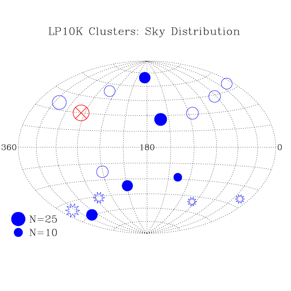
Figure 1.: Sky positions of the fifteen LP10K clusters. Filled circles represent clusters for which the mean redshift of the LP10K TF sample is $\leq 12,\!000\ {\rm km}\,{\rm s}^{-1}.$ Open circles represent clusters with mean TF sample redshift $12,\!000\ {\rm km}\,{\rm s}^{-1}\leq cz\leq 15,\!000\ {\rm km}\,{\rm s}^{-1},$ and starred symbols those with mean $cz>15,\!000\ {\rm km}\,{\rm s}^{-1}.$ The number of galaxies in the cluster TF sample is symbolized by the point size, as indicated by the key at the lower left. The “$\times$” enclosed by a circle shows the direction of the LG motion with respect to the CMB.

In each cluster I obtained $R$-band CCD imaging of 1–2 square degrees of sky centered on the cluster core. These moderately deep ($R\lower 2.15277pt\hbox{$\,\buildrel<\over{\sim}\,$}21.5$ mag) CCD frames were then analyzed using FOCAS, and all galaxies brighter than about $m_{R}=17.5$ were visually inspected for suitability as TF galaxies.

The skeptical reader might pause here and ask what “suitable” means in this context. Initially, it meant something rigorous such as “brighter than a certain apparent magnitude and more inclined than a certain minimum inclination.” I quickly learned that I could not afford to be so picky, however. If I wanted galaxies whose rotation would be detected, I needed to pick galaxies that were emitting a lot of H$\alpha$ radiation. The only way to ensure this was to choose objects primarily on morphological appearance: they had to look they had a lot of star formation going on. Basically, this means well-defined spiral structure, generally late-type morphology, and some visual evidence of Hii regions. Moreover, I couldn’t apply a single magnitude limit for all clusters; rather, I had to go much deeper in clusters with fewer bright, suitable spirals, in order to obtain a sufficient number of TF galaxies. This, I confess, is not a very rigorous selection procedure, but it was the one that had to be followed to make the program feasible.

Once the spirals were selected as described above, they were observed spectroscopically at the LCO 2.5 m or the Palomar 5 m telescopes. Long-slit spectra were acquired at about 2 Å resolution, in the portion of the spectrum containing H$\alpha$ out to $z=0.1$ Despite my efforts at preselecting objects that would exhibit H$\alpha$ emission, I suffered though many, many nondetections. This included objects with nuclear H$\alpha$ emission, fine for redshift purposes, but not extended enough to get a rotation velocity. This should serve as a cautionary warning to observers hoping to do deep, optical TF studies: hone your selection criteria in advance so you don’t waste too much large telescope time. Detectable, extended H$\alpha$ emission is by no means guaranteed from faint spirals.

Because I selected TF galaxies from new CCD imaging and not from a catalog, I didn’t know in advance what their redshifts would be, but I assumed they would usually be close to the nominal values of their parent clusters. This is where I got my second rude surprise (after nondetections): a large fraction ($\sim 30$–$40\%$) of the TF sample lay well in the background of the cluster. In the end, fully two-thirds of the galaxies with extended H$\alpha$ emission were found to have $cz>15,000\ {\rm km}\,{\rm s}^{-1},$ and a not insignificant number had $cz\approx 30,000\ {\rm km}\,{\rm s}^{-1}.$ I intend at a later date to explore the implications of these galaxies, which are perfectly good Tully-Fisher objects, for monopole distortions to the Hubble expansion, which is of considerable scientific interest. For the immediate goal of bulk flow on a 100 Mpc scale, of course, these objects were not especially useful. In Figure 1, the point type codes the median redshift of the TF sample. Note that the clusters with the greatest preponderance of high-redshift objects lie preferentially near the South Galactic Cap; this result merits further attention, as it could be indicative of very large-scale structure.

In the orginal survey plan, I hoped to obtain Fundamental Plane (FP) data for 15 ellipticals in each cluster to supplement, and provide an independent check on, the TF distances. Indeed, an auxiliary scientific goal of the survey was to use the spiral/elliptical cross-check as a test for environmental effects—significant E/S distance discrepancies that correlated with cluster properties would provide evidence for these. Unfortunately, the elliptical galaxy spectroscopic data is still very much in the reduction process, in the case of LCO ellipticals which I could observe using the du Pont telescope multifiber spectrograph, and are still to be acquired in the case of Northern sky ellipticals. If the LP10K elliptical results ever come out, it will probably be via a healthy amount of merging with other data sets. In hindsight, I can see that including ellipticals in the survey plan was a proverbial case of “biting off more than I could chew.” I say this not for the purpose of public self-flagellation but as a cautionary tale for ambitious postdocs contemplating a massive observational program. In any case, readers should keep in mind that the results presented in Papers I and II, and here, are based on Tully-Fisher data only.

3. Formulating the Optical TF Relation

3.1. Defining the TF Rotation Velocity

A key question that the LP10K survey data addressed was, “Given that we have rotation curve (RC) data, $V(R),$ for each galaxy, what particular velocity $V_{{\rm TF}}$ is it that enters into the TF relation?”. While similar questions arose in the older, HI-based TF surveys, where one had to extract a width from an unresolved 21 cm profile, the problem then was largely algorithmic. With long-slit spectroscopy, however, we have resolved data, and the issue of “what rotation velocity enters into the TF relation” becomes a physically meaningful one.

For LP10K I took the following approach. First, the RCs were fitted using a two-paremeter functional form:

$$V(R)=\frac{2V_{a}}{\pi}\tan^{-1}\left(\frac{R}{R_{t}}\right)\,.$$

The arctangent form approximates the canonical S-shaped rotation curve, but can also represent the quasi-linear RCs, still rising at the outermost point, that are frequently encountered. It is useful to refer to $V_{a}$ as the “asymptotic” velocity, and to $R_{t}$ as the RC scale length or “turnover radius.” It is important to bear in mind, however, that the velocity $V_{a}$ is not necessarily reached by the sampled RC, and may in fact not be reached at all, so its name, while evocative, is not rigorous. Note also that for a quasi-linear RC, only the ratio $V_{a}/R_{t}$ is well-determined from the fit. Still, bearing these caveats in mind, the arctan fit proved quite adequate for all LP10K galaxies.

The photometric data also yields a scale length for the galaxy, viz., $R_{e},$ in this case the effective exponential scale length (see Paper I for more detail on how this was computed; it was not from an exponential fit). With it, one can pose the question of “what is $V_{{\rm TF}}$” in this way: at how many exponential scale lengths should one evaluate the rotation curve $V(R)$ to get the best (lowest-scatter) TF relation? Let us parametrize this question by writing $V_{{\rm TF}}=V(f_{s}R_{e}),$ where the right side is evaluated from the arctan fit, and take $f_{s}$ as a free paramer. I like to write this in the following way:

$$V_{{\rm TF}}=\frac{2V_{a}}{\pi}\tan^{-1}\left(\frac{f_{s}}{x_{t}}\right)\,,$$

where $x_{t}\equiv R_{t}/R_{e}$ is a dimensionless shaper parameter which measures the ratio of the dynamical to luminous scale lengths of the galaxy. Roughly speaking, $x_{t}\ll 1$ is a classical S-shaped RC, with the flat part well sampled, while $x_{t}\lower 2.15277pt\hbox{$\,\buildrel>\over{\sim}\,$}1$ is a quasi-linear RC.

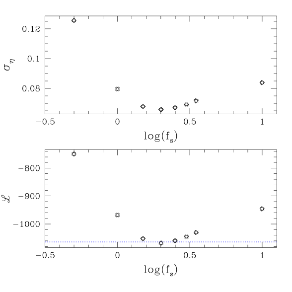
Figure 2.: The inverse TF scatter (top panel) and the fit likelihood statistic, ${\cal L}=-2\ln P({\rm data}|{\rm model}),$ plotted versus the value of $f_{s}.$ Both plots show a clear minimum (i.e., a best fit) at $f_{s}=2.0\pm 0.1.$

We next define the velocity width parameter, in the usual way, $\eta(f_{s})=\log(2V_{{\rm TF}})-2.5,$ and write the inverse TF relation $\eta(f_{s})=-e(M-D).$ This is a three-parameter TF relation, with slope $e$ and zero point $D$ supplemented by $f_{s}.$ The values of all the parameters can be determined by maximum likelihood (see Papers I and II), with absolute magnitude given by a simple Hubble Flow model (in the CMB frame). It is illustrative to do this for a range of fixed values of $f_{s},$ maximizing likelihood with respect to $e$ and $D$ at each value and obtaining a correponsponding TF scatter and fit likelihood. The results of this exercise are presented in Figure 2. The plot shows that the “correct” value of $f_{s}$—i.e., the one that minizes TF scatter—is quite tightly constrained at $f_{s}\approx 2.0.$ In particular, one sees that taking $f_{s}\gg 1,$ corresponding to taking $V_{{\rm TF}}=V_{a},$ leads to a poor TF relation. This is an important point, for it demonstrates that the canonical wisdom—that the TF relation involves the velocity on the flat part of the RC—is wrong. In Paper I a heuristic physical explanation for this effect is offered, but undoubtedly the correct explanation is much deeper, and I encourage theorists to delve more deeply into this issue.

3.2. A Surface Brightness Dependence of the TF Relation

Another galaxy property which turned out to enter into the TF relation was the effective surface brightness $I_{e}$ (calculated via the same method that produced the scale length $R_{e}$—see Paper I for details). Specifically, we can write the TF relation

$$\eta(f_{s})=-e(M-D)-\alpha\mu_{e}\,,$$

where $\mu_{e}$ is the magnitude equivalent of $I_{e}.$ When this was done, a small but statistically significant reduction in the TF scatter was found; the coefficient was found to be $\alpha\approx 0.05,$ which when combined with $e\approx 0.12$ leads to a power-law scaling relation of the form $V_{{\rm TF}}\propto I_{e}^{0.13}L^{0.3}.$ This relation is reminiscent of the FP relations for elliptical galaxies. The surface brightness dependence of the TF relation has significant implications for galaxy structure.

It is only fair to note here that my claim of an SB dependence of the TF relation is not universally accepted. Riccardo Giovanelli made the very good point at the conference that by introducing a scale length into the definition of velocity width, I may have induced a spurious SB dependence of the TF relation. My Shellflow colleague Stéphane Courteau has argued that the particular method I employ for determining $R_{e}$ and $I_{e}$ from the surface brightness profiles could produce the dependence, whereas in a more standard approach the dependence would not show up. As of this writing (8/31/99) these possibilities have not been fully investigated. I hope to study this issue more closely in the coming months with the Shellflow data, and in the meantime I encourage input from members of the community who have done such experiments with their own data.

3.3. The Intrinsic TF Scatter

The likelihood fits used in Papers I and II made it possible to constrain the individual contributions to the overall TF scatter: measurement errors and intrinsic scatter. Although the rotation velocity measurement errors were not well determined a priori, they can be separated from the intrinsic scatter because the TF error they induce scales as $\delta\eta\propto\delta v/v.$ (Photometric errors are fairly well determined, and are small in any case.) Thus, if one assumes a fixed velocity measurement error, the overall $\eta$ error $\propto V_{{\rm TF}}^{-1}.$ Using this model, I found that (i) the characteristic rotation velocity measurement error was $\sim 17\ {\rm km}\,{\rm s}^{-1},$ a reasonable value consistent with repeat observation comparisons; (ii) the observed decrease of TF scatter with increasing luminosity can be fully accounted for in this way—i.e., we are not required to assume the intrinsic TF scatter decreases with increasing luminosity—and (ii) the intrinsic TF scatter itself is $0.28\pm 0.07$ mag. This value is consistent with what was found by Willick et al. (1996) via an independent approach, and is also consistent with findings from the Shellflow survey (Courteau et al., this volume). Reproducing this level of scatter is an important challenge for galaxy formation theory.

4. On Bulk Flows

To determine the best-fitting bulk flow vector $\vec{v},$ I calculated absolute magnitude as $M=m-5\log[(cz-\vec{v}\cdot{\hat{\bf n}})/H_{0}]-25,$ and then maximized TF likelihood as before. Paper II gives many details about these fits, but the upshot is that the derived flow vector has an amplitude of $\sim 700\pm 300\ {\rm km}\,{\rm s}^{-1}$ in the direction quoted in the Abstract. The relevant question now is, what should we make of this? As those who heard my talk at the conference, or heard about it, already know, I no longer consider this result to be “correct.”

Unfortunately, this seems to have led to a perception that I am “disavowing my own data.” This is untrue. The data is perfectly good, or at least as good as it can be given the observational challenges described above. Rather, my point of view is that this result is noisy—the flow is detected at the $\sim 2.3\sigma$ level—and thus would require extensive corroboration to be accepted. Looking at the other data sets around—most of them presented at the Cosmic Flows workshop—the prevailing picture is one of convergence to the CMB frame on smaller scales. Most convincing to me, because I worked on it, are the Shellflow results, which clearly show convergence at 6000 km s^-1. Also very persuasive in this regard are the new supernova results presented by Adam Riess.

To believe the LP10K bulk flow result, then, I would have to accept that the Hubble flow converges to the CMB frame at 6000 km s^-1, and then starts drifting away from the CMB frame beyond this distance. This would be blatantly unphysical. By and large I harbor few prejudices about how the universe should behave, but I basically do believe that gravitational instability drives structure formation and flows, and that the universe approaches homogeneity on progressively larger scales. If this is true, and Shellflow and the other shallower surveys are correct, the LP10K flow result cannot be. That is not a disavowal of my own data, but quite basic and, I hope, sound scientific reasoning.

Acknowledgments.

First and foremost, I once again thank my friend and collaborator Stéphane Courteau for organizing this fantastic conference. I also thank Felicia Tam, a Stanford undergraduate, for invaluable assistance in reducing the LP10K data over the last two years.

References

Abell, G.O., Corwin, H.G., & Olowin, R.P. 1989, ApJS, 70, 1

Lauer, T.R., & Postman, M. 1994, ApJ, 425, 418 (LP)

Lynden-Bell, D., Faber, S.M., Burstein, D., Davies, R.L, Dressler, A.,Terlevich, R., & Wegner, G. 1988, ApJ, 302, 536

Mathewson, D. S., Ford, V. L, & Buchhorn, M. 1992, ApJS, 81, 413

Willick, J. A. 1990, ApJ, 351, L5

Willick, J. A., Courteau, S., Faber, S. M., Burstein, D., Dekel, A., & Kolatt, T. 1996, ApJ, 457, 460

Willick, J.A. 1999a, ApJ, 516, 47 (Paper I)

Willick, J.A. 1999b, ApJ, in press (Paper II, astro-ph/9812470)