Panel Review: Reconstruction Methods and the Value of $\beta$

Abstract

The closely related issues of (1) reconstructing density and velocity fields from redshift survey and distance indicator data and (2) determining cosmological parameters from such data sets are discussed. I focus on possible explanations for the discrepant values of $\beta\equiv\Omega^{0.6}/b$ resulting from analyses that employ various reconstruction methods. Although no firm conclusions are reached, possible routes towards resolution of these discrepancies are suggested by the discussion.

Physics Department, Stanford University, Stanford, CA 94305-4060

1. Introduction

The original charge to our panel, which consisted of myself, Marc Davis, Avishai Dekel, and Ed Shaya, was to discuss “Reconstruction Methods.” To narrow the discussion, we decided in advance to concentrate on the problem of deriving $\beta$ from comparison of redshift survey and distance indicator data. This seemed appropriate given the panel membership: all of us have worked on this problem, and together we span the spectrum of results, from low values of $\beta$ suggestive of a low density ($\Omega_{M}\sim 0.2$) universe to high values consistent with $\Omega_{M}=1.$

While it may appear that we have strayed from the theme of “reconstructions,” $\beta$-determination is, in fact, closely linked with how we reconstruct the underlying velocity and density fields from the observable data. I clarify this point in § 2 below. In § 3, I review recent results for $\beta$ from peculiar velocities and consider possible explanations for their wide variance. I conclude in § 5 with a brief look to the future of the subject.

2. Reconstructions and $\beta$

Our theoretical formulation of cosmic dynamics involves the mass overdensity field $\delta_{\rho}(\vec{r})$ and the peculiar velocity field ${\vec{v}_{p}}(\vec{r}).$ Linear gravitational instability theory tells us that these fields obey the simple relation $\nabla\cdot{\vec{v}_{p}}=-f(\Omega_{M})\delta_{\rho},$ where $f(\Omega_{M})\approx\Omega_{M}^{0.6}.$

Such continuous fields are abstract mathematical constructs; reality is more complex. Discrete entities—galaxies—sparsely populate the universe, and we measure their redshifts and estimate their distances. Reconstruction Methods are the numerical algorithms we employ to turn these real-world data into representations of the underlying fields $\delta_{\rho}$ and ${\vec{v}_{p}}.$

Several obstacles stand between the measurements and successful reconstruction of the density and velocity fields. First, there is biasing: how is the galaxy overdensity $\delta_{g}$ related to the desired $\delta_{\rho}?$ In the oft-used if oversimplistic linear biasing paradigm $\delta_{g}=b\,\delta_{\rho},$ and the linear velocity-density relation becomes $\nabla\cdot{\vec{v}_{p}}=-\beta\delta_{g}.$ To the extent linear biasing and linear dynamics hold, only $\beta,$ not $\Omega_{M},$ is measureable by this method. Incorporating “realistic” models of biasing—and it is by no means clear that such models exist yet—presents another challenge to reconstruction methods. Reconstruction of ${\vec{v}_{p}}$ is if anything an even more daunting task: we estimate only the radial component of this field, at discrete, irregularly distributed positions, with large errors that grow linearly with distance.

We cannot invoke the theoretical velocity-density relation, and thus measure $\beta,$ until we have reconstructed the underlying fields. If our reconstructions of $\delta_{g}(\vec{r})$ and/or ${\vec{v}_{p}}(\vec{r})$ are flawed, we’ll get the wrong value of $\beta.$ And given the difficulties such reconstructions face, errors in $\beta$ are, perhaps, inevitable at this early stage in our understanding.

Figure 1 summarizes the relationship between reconstruction methods and $\beta$-determination. The box at the bottom concerns the nature of the comparison by which $\beta$ is obtained. If one reconstructs $\vec{v}_{p}$ from the peculiar velocity data and compares its divergence with $\delta_{g}$ from redshift survey data, one is doing a density-density (d-d) comparison. Alternatively one can reconstruct ${\vec{v}_{p}}(\vec{r})$ from redshift survey data (for an assumed value of $\beta$), using the integral form of the linear-velocity density relation, and compare with observed radial peculiar velocity estimates. This is known as the velocity-velocity (v-v) comparison. The distinctions between the two approaches are subtle but important, as discussed below.

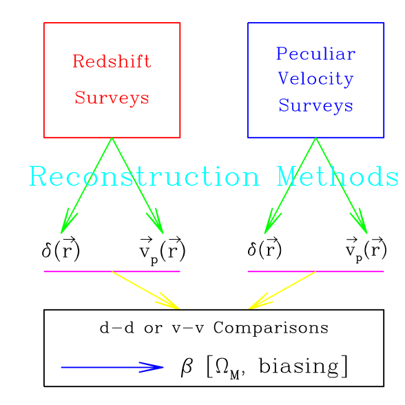
Figure 1.: A schematic representation of the relationship between input data, reconstructions, and derivation of cosmological parameters.

3. Discrepant $\beta$ Values, and Possible Explanations for Them

It was not until the early 1990s that measuring $\beta$ by comparing peculiar velocity and redshift survey data became a realistic goal. The advent of full-sky redshift surveys—notably those based on the IRAS point source catalog—and large, homogeneous sets of Tully-Fisher (TF) and related data were the key developments. The earliest attempt was that of Dekel et al. (1993), the so-called “POTIRAS” comparison. In this procedure the velocity field is reconstructed using the POTENT algorithm, and its divergence compared with the galaxy density field from IRAS (a d-d comparison). Dekel et al. (1993) found $\beta_{I}=1.29,$ a value widely taken as support for the then-popular Einstein-de Sitter paradigm. The POTIRAS analysis has since been redone with much improved peculiar velocity data, with the result $\beta_{I}=0.89\pm\ 0.1$ (Sigad et al. 1998), still consistent with a critical density universe unless IRAS galaxies are strongly anti-biased.

Between the first and second POTIRAS papers, a number of studies, based on the v-v comparison, arrived at markedly lower values of $\beta_{I}.$ Shaya, Tully, & Peebles (1995) estimated $\Omega_{M}=0.17\pm 0.1$ ($\beta_{I}\approx 0.35$ if IRAS galaxies are unbiased) using the Least Action Principle to predict peculiar velocities. Willick et al. (1997) and Willick & Strauss (1998) used the VELMOD method to find $\beta_{I}=0.5\pm 0.06.$ The above results were obtained from TF data; an application of similar methods to more accurate (but far more sparse) supernova data yielded $\beta_{I}=0.4\pm 0.1$ (Riess et al. 1998). (This list is not exhaustive, and apologies are due to authors not cited; my aim is illustrative rather than comprehensive.)

Thus, it appears that a somewhat bimodal distribution of $\beta$ values has emerged. The d-d, POTIRAS method produces $\beta_{I}$ close to unity; the v-v comparisons, several based on the same redshift and velocity samples as POTIRAS, yield $\beta_{I}\sim 0.5.$ Neither the d-d nor the v-v comparison is inherently more valid; both are firmly grounded in linear gravitational instability theory. What, then, could be the cause of the discrepancies?

Neither the panelists nor the conference participants arrived at a satistfactory answer to this question. However, the following list of possible explanations proved to be fertile ground for discussion. The list is accompanied by my own (biased) commentary on the salience of each explanation.

• Malmquist bias. This famous statistical effect has long been invoked as a cause of discrepant conclusions in astronomy. In fact, it is now a non-issue. Methods are now available for rendering Malmquist and related biases inconsequential; see Strauss & Willick (1995) for a detailed discussion.

• Nonuniverality of the TF and other distance-indicator relations. Another non-issue. It is easy to make the general argument—nonuniversal distance indicators imply spurious peculiar velocities—but there is little or no evidence implicating such effects in the $\beta$ problem.

• Calibration Errors in Peculiar Velocity Datasets. Such errors may indeed be present; new results from the Shellflow project (see the paper by Courteau in these proceedings) suggest that the widely used Mark III catalog has across-the-sky calibration errors. However, these errors affect mainly bulk flow estimates, not the value of $\beta_{I}$ (see Willick & Strauss 1998 for a clear demonstration of this).

• Non-trivial biasing. It is now widely believed that biasing is not only nonlinear, but stochastic and nonlocal (see the panel review by Strauss in these proceedings). If so, it is perhaps unsurprising that different approaches produce different results, as they may in fact be measuring different things. This argument may well contain a kernel of truth, but I am not convinced it is the whole story. I was impressed by the work of Berlind, Narayanan, and Weinberg on this subject (see their contributions to the proceedings), which shows that for all but the most contrived models of biasing, the value of $\beta$ one obtains is relatively insensitive to methodology.

• The density-density versus the velocity-velocity comparison. This, I think, is the central issue. We may be asking too much of our distance indicator data when we use them to derive the full 3-D velocity field and its derivatives, as is required for the d-d comparison. In the v-v comparison, by contrast, the distance indicator data is used essentially in its raw form; only the redshift survey data, which is intrinsically more accurate, is subject to complex, model-dependent manipulation. From this perspective, I would argue that the low values, $\beta_{I}\approx 0.4$–$0.5,$ that have come out of the v-v analyses are more likely to be correct.

4. A Quick Look to the Future

If we learned anything from our panel discussion, it was the usual lesson: better data will help. Fortunately, some already exist, and more are on the way. The Surface Brightness Fluctuation (SBF) data of Tonry and collaborators (see Tonry’s paper in these proceedings) are now available for comparison with the IRAS redshift data; preliminary results are reported by Blakeslee in these proceedings. SBF distances are considerably more accurate than TF distances and promise a much higher-resolution look at the velocity field. Adam Riess reported new, and also very accurate, SN Ia distances for nearby galaxies. The extant TF data are not likely to increase dramatically in the short term, but will be recalibrated by the Shellflow program, and perhaps the different TF data sets (Mark III, SFI, Tully’s Catalog) will be merged into a larger, homogeneous catalog. In the longer term ($\sim 5$–10 years), they will be supplanted by much larger and more uniform TF data sets that will emerge from the wide-field infrared surveys currently under way, 2MASS and DENIS (see the contributions by Huchra and Mamon in these proceedings).

I draw yet another lesson from our panel discussion: we have not yet fully developed the analytical methods needed to deal with nonlinearities in the universe, both dynamical and biasing-related. In this regard I would encourage theorists to address the problem of, how, given a particular biasing model, do we predict the peculiar velocity field from redshift survey data, taking full account of nonlinear dynamics? When reliable methods are developed for doing this, and tested against N-body simulations, we will be able to fully exploit the improved peculiar velocity data sets of the future.

Acknowledgments.

I thank my fellow panel members, Marc Davis, Avishai Dekel, and Ed Shaya, for stimulating discussions.

References

Dekel, A., Bertschinger, E., Yahil, A., Strauss, M., Davis, M., & Huchra, J. 1993, ApJ, 412, 1

Riess, A.G., Davis, M., Baker, J., & Kirshner, R.P. 1997, ApJ, 488, L1

Shaya, E.J., Peebles, P.J.E., & Tully, R.B. 1995, ApJ, 454, 15

Sigad, Y., Eldar, A., Dekel, A., Strauss, M.A., & Yahil, A. 1998, ApJ, 495, 516

Strauss, M. A., & Willick, J. A. 1995, Phys. Rep., 261, 271

Willick, J.A., Strauss, M.A., Dekel, A., & Kolatt, T. 1997, ApJ, 486, 629

Willick, J.A., & Strauss, M.A. 1998, ApJ, 507, 64