THE EVOLUTION OF EARLY-TYPE GALAXIES IN DISTANT CLUSTERS II.: INTERNAL KINEMATICS OF 55 GALAXIES IN THE $z=0.33$ CLUSTER CL1358+62¹

Abstract

We define a large sample of galaxies for use in a study of the fundamental plane in the intermediate redshift cluster CL1358+62 at $z=0.33$. We have analyzed high resolution spectra for 55 members of the cluster. The data were acquired with the Low Resolution Imaging Spectrograph on the Keck I 10m telescope. A new algorithm for measuring velocity dispersions is presented and used to measure the internal kinematics of the galaxies. This algorithm has been tested against the Fourier Fitting method so the data presented here can be compared with those measured previously in nearby galaxies.

We have measured central velocity dispersions suitable for use in a fundamental plane analysis. The data have high $S/N$ and the resulting random errors on the dispersions are very low, typically $<5\%$. Uncertainties due to mismatch of the stellar templates has been minimized through several tests and the total systematic error is of order $\raise 1.29167pt\hbox{$\scriptscriptstyle\sim$}5\%$. Good seeing enabled us to measure velocity dispersion profiles and rotation curves for most of the sample and although a large fraction of the galaxies display a high level of rotation, the gradients of the total second moment of the kinematics are all very regular and similar to those in nearby galaxies. We conclude that the data therefore can be reliably corrected for aperture size in a manner consistent with nearby galaxy samples.

1. Introduction

Scaling relations have been extensively used to measure the evolution of galaxies to redshifts of $z\sim 1$. However, without mass scales, provided by measurements of rotation curves or line-widths, it is impossible to extract the evolution of galactic $M/L$ ratios from that of the underlying luminosity function. The explicit use of galaxy masses, in the fundamental plane (Faber et al. (1987); Djorgovski & Davis (1987)), or the Tully-Fisher relation (Tully & Fisher (1977)), makes these scaling relations extremely powerful tools for measuring galaxy evolution.

The fundamental plane (FP) is useful for quantifying the luminosity evolution of early-type galaxies in distant clusters. It is an empirical relation between effective radius, velocity dispersion, and surface brightness, for early-type galaxies. In a study of 10 nearby clusters Jørgensen et al. (1996) found

$$\log r_{e}\propto 1.24\log\sigma-0.82\log\langle I\rangle_{e},$$ (1)

with an rms scatter of $\pm 0.084$ in $\log r_{e}$ (a 21% distance uncertainty). The virial theorem and homology imply

$$\log{M\over L}\propto 2\log\sigma-\log r_{e}-\log\langle I\rangle_{e}$$ (2)

The implication is that the mass-to-light ratio is a function of structural and kinematical observables (Faber et al. (1987)), such that

$$M/L_{V}\propto r_{e}^{0.22}\sigma^{0.49}.$$ (3)

The scatter in Coma of 23% in $M/L_{V}$ (Jørgensen et al. (1993)), for a given $\sigma$ and $r_{e}$, suggests a small scatter in age for a given $\sigma$ and $r_{e}$ (Prugniel & Simien (1996)). It has been postulated that systematic departures from homology exist along the fundamental plane (e.g., Ciotti, Lanzoni, & Renzini (1996)), but no satisfactory model has been created to explain both the slope, and the low scatter of the scaling relation. Evolution of the fundamental plane zero-point, slope, and scatter can provide critical insight into the evolution of stellar populations of early-type galaxies and may shed light on the origin of the fundamental plane itself.

In a pioneering effort, Franx (1995) used fundamental plane observations in A665 ($z=0.18$) to detect the evolution of stellar populations in early-type galaxies. van Dokkum & Franx (1996) continued this technique with early-type galaxies in CL0024+16 ($z=0.39$) and measured evolution consistent with the passive evolution of stellar populations which formed at very high redshift. More recently, Kelson et al. (1997) extended fundamental plane measurements to small samples in CL1358+62 at $z=0.33$, and MS2053–04 at $z=0.58$. Their results confirmed the evolution in the fundamental plane zero-point with redshift. van Dokkum et al. (1998b) have now extended fundamental plane measurements to $z=0.83$, and have constrained both the formation epoch of early-type galaxies and $\Omega$. Other authors have also used the elliptical galaxy scaling relations to constrain galaxy evolution and cosmology as well (e.g., Schade et al. (1997); Ellis et al. (1997); Ziegler & Bender (1997); Bender et al. (1998); Pahre (1998)), also finding that E/S0s in clusters are uniformly old.

Both van Dokkum & Franx (1996) and Kelson et al. (1997) suggested that the FP tilt may have evolved between $z=0.33\hbox{-}0.58$ and the present epoch, such that low-mass early-types are younger than their high-mass counterparts. Their data also indicated that the scatter was comparable to the nearby FP (Jørgensen et al. (1993); Kelson et al. (1997)). However, their samples were simply not large enough to accurately determine the slope or scatter in the fundamental plane at intermediate redshifts. Kelson et al. (1997) also found that the velocity dispersions of two E+A galaxies were low ($\sigma\sim 100$ km/s). Are such low velocity dispersions typical, and are these galaxies rotationally supported, such as would be expected for disk-dominated systems (e.g., Franx (1993))?

In this paper we describe the data and reduction procedures used to determine the internal kinematics of a large sample of galaxies in the cluster CL1358+62. The HST data, from which the sample was selected, are described in Kelson et al. (1999a) and van Dokkum et al. (1998a). Extensive Keck spectroscopy has now enabled us to measure velocity dispersions, dispersion profiles, and many absorption line rotation curves, for a homogeneous sample of cluster members. In §2, we report on the sample selection for the spectroscopy. The observations and data reduction procedures are briefly discussed in §3. The stellar templates are prepared in §4. Our method for deriving velocity dispersions using a direct fitting method is introduced in §5. In §6, we test the results against other velocity dispersion routines. In §7, we discuss the strategy for selecting the best template and investigate the magnitude of template mismatch. In §8, we discuss the aperture corrections required to place our velocity dispersions on the same system as the Jørgensen et al. (1996) database, and use the spatially resolved kinematics to compare the CL1358+62 members with nearby early-type galaxies. Lastly, sources of error, both random and systematic, are discussed in §9.

2. Sample Selection

We are currently studying, in detail, the galaxy populations of three clusters, CL1358+62 ($z=0.33$), MS2053–04 ($z=0.58$), and MS1054–03 ($z=0.83$), selected from the Einstein Medium Sensitivity Survey (Gioia et al. (1992)). Determining membership is critical for studying any cluster population. Fabricant et al. (1991) and Fisher et al. (1998) have recently collected several hundred redshifts in a $10^{\prime}\times 11^{\prime}$ field around CL1358+62; the Fisher et al. (1998) sample is more than 80% complete at $R\leq 21$ mag.

This field was targeted for extensive imaging with the HST WFPC2. A two-color mosaic of the cluster CL1358+62 covering $64\,{\mathchoice{\vbox{\vbox{\hrule height=0.2pt\hbox{\vrule width=0.2pt,height=6.0pt\kern 6.0pt\vrule width=0.2pt} \hrule height=0.2pt}}}{\vbox{\vbox{\hrule height=0.2pt\hbox{\vrule width=0.2pt,height=6.0pt\kern 6.0pt\vrule width=0.2pt} \hrule height=0.2pt}}}{\vbox{\vbox{\hrule height=0.1pt\hbox{\vrule width=0.1pt,height=4.2pt\kern 4.2pt\vrule width=0.1pt} \hrule height=0.1pt}}}{\vbox{\vbox{\hrule height=0.1pt\hbox{\vrule width=0.1pt,height=3.0pt\kern 3.0pt\vrule width=0.1pt} \hrule height=0.1pt}}}}\,\,^{\prime}$ was constructed using 12 pointings. Of the Fisher et al. (1998) database, 194 spectroscopically confirmed cluster members fall within the field of view of the HST imaging. From this large catalog, we selected a sample for detailed study with the Low Resolution Imaging Spectrograph (LRIS; Oke et al. (1995)) at the W.M. Keck Observatory. The high resolution of the HST imaging allows us to derive structural parameters with the accuracy needed for the fundamental plane (Kelson et al. 1999a ).

From the catalog of cluster members within the HST mosaic, we randomly selected galaxies down to $R<21$ mag. As is discussed in more detail in Kelson et al. (1999a), the $R$-band selected sample contains mostly early-type systems, ranging from ellipticals to early-type spirals. Our sample was constructed without regard for morphological information, contrary to most low redshift samples. The selection was performed with an effort to efficiently construct multi-slit plates for LRIS. We used three masks, with different position angles on the sky. During the designing of the multi-slit masks, we utilized the apparent morphologies of several galaxies for major-axis positioning, without impacting the selection criteria. The three mask designs overlap in the core of the cluster, and so the sample is concentrated towards the cluster center. A total of 67 slitlets were allocated for the three masks.

In Figure 1, we show the color-magnitude diagram for the spectroscopically confirmed cluster members within the HST mosaic. At the redshift of the cluster, $L^{*}$ corresponds to $R\sim 20.1$ mag (adopting the $M/L_{V}$ evolution as measured by Kelson et al. (1997)). There is clearly a tight color-magnitude relation in the cluster, as shown by van Dokkum et al. (1998a). The entire catalog of spectroscopically confirmed cluster members within the HST mosaic is shown by the circles, and those selected for fundamental plane analysis are shown by the filled circles. As can be seen in the figure, the fundamental plane sample fairly represents the cluster population, minus the very bluest and faintest objects (van Dokkum et al. 1998a ).

Fisher et al. (1998) found 108 members brighter than $R=21$ mag within the HST mosaic. Our high-resolution spectroscopic sample contains 52 of them. Since three cluster galaxies fainter than the magnitude limit were added, the total number of the sample presented here is 55. Two of these galaxies were observed using more than one slit-mask. Eight overlap the sample of Kelson et al. (1997).

This high-resolution sample of cluster members contains mostly spectroscopically early-type galaxies, a few E+A galaxies, and a few galaxies fainter than $R=21$ mag. The E+A galaxies are defined by $\rm(H\delta+H\gamma+H\beta)/3>4$ Å and [OII] 3727 Å $<5$ Å (Fisher et al. (1998)). The E+A fraction in our high-resolution spectroscopic sample is consistent with the fraction Fisher et al. (1998) found for the cluster, about 5%. By estimating the mass scales for these galaxies, we hope to constrain the relationship between the Butcher-Oemler effect (e.g., Butcher & Oemler (1978); Dressler & Gunn (1983); Caldwell & Rose (1997, 1998)) and the histories of “normal” cluster members (e.g., Franx (1993); Kelson et al. (1997)).

3. Observations and Data Reduction

In May 1996 we obtained high $S/N$ two-dimensional spectra in the field of CL1358+62. The data were acquired at the Keck I 10m telescope on Mauna Kea using LRIS with the three multi-slit aperture plates. The first two were exposed for 8100 s, and the third for 7400 s. We used the 900 mm^-1 grating, with a dispersion of approximately 0.85 Å per pixel. The restframe coverage was typically $\scriptscriptstyle\sim$4100 Å to $\scriptscriptstyle\sim$5200 Å. The seeing was typically 0^′′.75 to 0^′′.8 (FWHM). The slitlet widths were 1^′′.05, resulting in a typical resolution of $\sigma_{i}\approx 1.2$ Å ($\scriptscriptstyle\sim$60 $\rm km\,s^{-1}$). Some slitlets were “tilted” with respect to the primary axis of the slit-masks, to align them along galaxy major-axes. These slitlets have broader projected widths, and leading to slightly poorer spectral resolution. The treatment of the resolution is discussed explicitly in §4.

For the purposes of efficient and accurate extraction of one- and two-dimensional spectra, a new set of FORTRAN procedures was created. These subroutines are collected in a stand-alone package called Expector. Expector’s primary functions are that of flat-fielding, rectifying, and wavelength calibrating two-dimensional multi-slit spectroscopic data. Expector can be used trivially for long-slit reductions as well.

3.1. Preprocessing

Some initial processing is required before execution of Expector. The over-scan and bias-frame subtraction was done in IRAF. Cosmic-rays were rejected using median filtering, with a search algorithm for extended sharp objects. Care was taken to not degrade galaxy, or night sky features in the removal of cosmic-rays. Next, the camera, or “$y$”-distortion was determined by tracing the slit boundaries. This distortion was removed from the flat-field images and the cosmic-ray cleaned, bias-subtracted data frames.

The next steps involved flat-fielding the data, which requires several stages. First, the spectral dome-flats were normalized, on a slitlet-by-slitlet basis. The normalization occurs in both the $x$ and the $y$ directions and produces two output images: a two-dimensional pixel-to-pixel flat-field, and a one-dimensional column vector which represents the (multi-slit) slit function. After the first pass of the normalization procedures, re-normalized columns are medianed to produce a column vector which is output as the slit function. The pixel-to-pixel flat-field also contains a map of the fringing. For the data presented here, however, fringing is negligible. This processing of the flat-fields requires that the $y$-distortion be removed beforehand, so that the individual two-dimensional spectra are aligned with the dispersion axis of the CCD.

The data frames are divided by the pixel-to-pixel flat-fields. Tests using spectra extending to $\sim 9500$ Å showed that this step can be effective in removing fringing. Next, the one-dimensional slit functions are shifted (in the $y$ direction), such that the slit edges match those in the data frames. These shifts are required if the slit edges in the CCD images of the flat-fields are not registered with the slit edges in the data frames. Finally, the columns in the data frames are divided by the shifted slit functions. Each mask has its own set of flat-fields, in order to best match the spectral coverage of each pixel, and to match the individual slit functions.

3.2. Rectification and Wavelength Calibration

The two-dimensional multi-slit images were rectified and wavelength calibrated by Expector using the night sky lines ([O I], Na I, and OH). A single $2048\times 2048$ multi-slit image can be fully rectified, wavelength calibrated, and rebinned, for example, in just a few minutes on a DEC Alpha processor. We summarize the procedures below. The interested reader can find more details in Kelson (1998).

The technique for rectifying two-dimensional spectra uses Fast Fourier Transforms and efficient cross-correlations to measure the pixel shifts between regions of sky (or lamp) lines from image row to image row. Thus, our method does not rely on centering algorithms to fix the positions of individual lamp, or night sky, emission lines. The shifts, in pixels, between adjacent CCD rows are measured as a function of wavelength, by performing the cross-correlations in subsections of each spectrum, divided along the dispersion direction. We fit a two-dimensional polynomial to the shifts as a function of $(x,y)$ position, and use this polynomial to align all the rows to a common coordinate (wavelength) system. The typical rms scatter about the fit for these rectification transformations is a few millipixels, with several tens of millipixels in the worst (tilted) cases. This method for rectifying two-dimensional spectra is extremely accurate and computationally economical due to its maximal use of the available data.

Because the rectification aligns all the CCD rows, within a given spectrum, one only needs to determine the wavelength solution for a single row (or average of several, in order to improve the $S/N$). Expector’s automated wavelength calibration routine can use LRIS lamp lines, or the night sky emission lines. The algorithm quickly finds the emission peaks, measures the FWHM of each peak non-parametrically, and defines the center of each line to be the average of the two half-power points. When calibrating spectra using night-sky emission lines, the algorithm quickly finds an approximate central wavelength using cross-correlations, and then identifies triplets of P1 and P2 OH lines using ratios of spacings between sky lines. After an initial determination of a low-order wavelength solution, more lines are identified and used to refine the solution.

We chose to fit a fifth order Legendre polynomial for the dispersion solutions. The rms scatter about the fit was typically $\pm 0.01$-$0.03$ Å, though somewhat worse for tilted slitlets due to the increase in the width of the lines. Comparison lamp spectra were used to test the validity of the wavelength solution as derived from the night sky emission. The sky lines had equivalently low rms scatter about the lamp solutions, once the zero-point in the wavelength calibration had been corrected. We opted for a dispersion solution derived directly from the night sky, using emission lines down to 5224 Å.

Each slitlet was rebinned logarithmically to a common wavelength range, by chaining the rectification transformations and dispersion solutions together. This step involves a single interpolation in the $x$ (wavelength) direction. The output images are extra wide to accommodate the staggering of the slitlets in the dispersion direction, and flux was conserved in the rebinning of each image. Note: the data were rebinned only once in the $y$ direction of the CCD and once in the $x$ direction. The exposures were then averaged, weighting inversely by the expected noise, including the noise in the sky and galaxies, as well as the read noise in the amplifier. Background subtraction was carried out in a manner similar to long-slit reductions, in which the sky spectrum at the location of a galaxy is interpolated using the observed sky on either side. Residuals around strong night sky lines, such as 5577 Å, and 6300 Å, were interpolated over, though this step was performed largely for cosmetic reasons.

Spectra for the galaxies were extracted by summing five CCD rows. The mean $S/N$ ranges from 10 to 80 per Å, with a median of $\scriptscriptstyle\sim$35 per Å. This high $S/N$ allowed us to sum the image rows directly, rather than optimally, which would complicate the determination of the effective aperture of the extraction. The spectra themselves are shown in Figure 2. The 5 row aperture, $1\hbox{${}^{\prime\prime}$\hbox to0.0pt{\hss.}}08\times 1\hbox{${}^{\prime\prime}$\hbox to0.0pt{\hss.}}05$, is equivalent to a circular aperture of diameter 1^′′.23 (Jørgensen et al. (1995)). In an $\Omega=0.5$, $H_{0}=65\ \hbox{$\rm km\,s^{-1}$}\rm\,Mpc^{-1}$ universe, this corresponds to a circular aperture of diameter $\scriptscriptstyle\sim$5.5 kpc (or equivalently $11^{\prime\prime}$ at the distance of Coma). Slitlets tilted by $45^{\circ}$ have an effective aperture 19% larger in diameter.

4. Preparation of Template Spectra

Because these galaxies are at cosmological distances, one must process stellar template spectra with care in order to ensure that they have the the same restframe instrumental resolution as the galaxy spectra (Franx (1993)). For nearby galaxies, this is obviously not a problem, as the same instrumental setup can be used to obtain both the stellar and galactic spectra. However, for high-$z$ objects, template spectra cannot be observed with the same instrumental setup and one must carefully model the resolution of the galaxy spectra. The stellar spectra must be treated with extra caution as well if their resolution is similar to that in the galaxy spectra (see Franx (1993); van Dokkum & Franx (1996)). The spectra of template stars must be convolved by a kernel to match the point-spread function of the galaxy spectra.

Using LRIS during twilight in May and August 1996, we performed long-slit spectroscopy of several late-type stars (G and K stars), listed in Table 1. The 1200 mm^-1 grating was used, providing spectral coverage from 4000 Å to 5300 Å, with a dispersion of approximately 0.64 Å per pixel. These resulted in spectra with higher resolution that that of our galaxy spectra (see §4.3). The telescope was moved in a raster pattern to expose the star across the full width of the slit at several spatial positions. It is important to fill the width of the slit (0^′′.7), such that the spectral resolution is limited by the slit width, and not by the seeing. These data were also bias-subtracted, flat-fielded, rectified, and wavelength-calibrated. The extracted stellar spectra have very high $S/N$, several hundred per pixel.

4.1. The Wavelength Calibration of the Stellar Spectra

The stellar spectra were wavelength calibrated using a sparse sample of comparison lamp lines in the blue (mostly Ar and Hg). A dearth of bright lamp lines in the blue led us to test the validity of the dispersion solution when applied to the stellar long-slit spectra. We performed a cross-correlation of a high resolution solar spectrum, with the twilight and template spectra, over small, 100 Å bins, to provide an independent check on the wavelength calibration. There was a high-order systematic trend with wavelength, such that there was a net velocity difference between the red and blue sides of the stellar spectra. The wavelength calibration derived from the internal lamps was in error, by about $30$ $\rm km\,s^{-1}$ peak-to-peak, from blue to red, in the May stellar spectra, and about $40$ $\rm km\,s^{-1}$ peak-to-peak in the August stellar spectra — equivalent to a non-linear stretching of about 1 pixel. This can be attributed to the dearth of available lamp lines in the blue, coupled with centering errors in asymmetric arc profiles, especially in the August lamp data. Using this cross-correlation information, we rebinned the raw template spectra to the proper dispersion solution.

4.2. Spectral Resolution of the Template Stars

We determined the instrumental broadening in our stellar spectra in two complementary ways. Initially, the resolution of these stellar spectra was determined using the widths of the comparison lamp lines. For the May stellar spectra, the $\sigma$ widths of these lines are shown in Figure 3 as crosses. However, the internal lamps in LRIS do not necessarily illuminate the spectrograph in the same manner as the sky. Thus, we wished to compare the arc line widths with the resolution of the stellar spectra themselves. We were able to measure the intrinsic broadening in the stellar spectra by comparing them with a high-resolution solar spectrum.

Using the Fourier Fitting Method (Franx, Illingworth, & Heckman (1989)), we determined the broadening required to match the high-resolution solar spectrum to the spectrum of the twilight sky. The typical resolution in the May 1996 stellar spectra was $\scriptscriptstyle\sim$50 km/s. These Fourier Fitting Method results are shown as open circles in Figure 3, for direct comparison with the $\sigma$ widths of the lamp lines. The two methods give similar broadening profiles as a function of wavelength. This comparison gives us confidence that the resolution is well-determined. We also used the high-resolution solar spectrum to find the instrumental broadening in the stellar spectra themselves and found consistent results, except around the Balmer lines, where the solar spectrum is clearly not a good match to the later-type stars.

The August 1996 stellar template spectra were taken after an upgrade of LRIS, in which a new CCD, field-flattener, and dewar were installed. The lamp spectra taken at this time have strongly asymmetric profile shapes, probably due to the internal illumination overfilling the grating (Gillingham 1996, private communcation ). Thus, the spectrograph’s resolution of the sky (and galaxies) may not be well-described by the arc line profiles. Therefore, we used the high resolution solar spectrum again, to directly measure the instrumental broadening in the August stellar spectra. There was no twilight spectrum from August, but the spectrum of the G5IV template star is close in type to the solar spectrum, thus minimizing any problems with template mismatch in the determination of the resolution. At 4500 Å, the high-resolution spectrum implies an instrumental broadening in the HD5268 spectrum of 45 $\rm km\,s^{-1}$, while the lamp line widths yield 55 $\rm km\,s^{-1}$.

If the resolution derived from the August 1996 arc spectra were to have been adopted instead of that derived from the solar spectrum comparison, we would have incurred a $-3\%$ error in velocity dispersion at $\sigma=100$ $\rm km\,s^{-1}$. At $\sigma=300$ $\rm km\,s^{-1}$, this error is only $-0.3\%$. Thus, the effect on the slope, $\alpha$, of the fundamental plane, $\log{r_{e}}\propto\alpha\log\sigma+\beta\log\langle I\rangle$, would have been to increase the coefficient of $\log\sigma$, by $\Delta\alpha\approx+0.02$.

For both the May and August stellar spectra, we adopted the resolution determined from the high resolution solar spectrum.

4.3. The Instrumental Resolution of the Galaxies

The night sky lines enabled us to measure the variation in instrumental broadening as a function of wavelength, for each of the CL1358+62 slitlets. However, care must be taken since blended sky lines can bias the measurement of the instrumental broadening. Therefore, the spectrograph resolution was measured using a list of bright night-sky lines, chosen such that they are unblended at our resolution. In particular, we used the emission lines at 5577 Å, 6300 Å, 6364 Å, and an array of OH P1 lines, all of which are listed in Table 2 (see Osterbrock et al. (1996)). The OH P1 lines are close blended doublets, which, for our instrumental setup, impacts our estimate of the resolution at levels smaller than $<0.5\%$. The effect is negligibly small for our velocity dispersion measurements. We also note that the profiles of these sky lines were well fit by pure Gaussians.

The sky line widths vary as a function of wavelength and position across the CCD. We fit third order polynomials to the sky-line widths as a function of wavelength, for each slitlet. The variation in template resolution with wavelength was also modeled with a third order polynomial. The final, prepared template spectra were generated by convolving the stellar spectra using a Gaussian with a $\sigma$ width determined by the quadrature difference between the two resolution polynomials. This procedure was tested by measuring the effective resolution of the prepared template spectra using the high-resolution solar spectrum. The effective resolution of the prepared templates agreed with the sky line widths to within a few percent.

Figure 4 shows sky line widths as a function of wavelength for each of the CL1358+62 galaxy slitlets in the second mask. The circles show the measured widths of the sky lines in $\rm km\,s^{-1}$, while the solid lines show the polynomial fit to these data. The dashed and dotted lines show the polynomial representation of the template spectral resolution for the May and August stellar spectra (see, e.g., Figure 3). The resolution for each slitlet was determined from the combined spectra of three exposures per mask. The widths of the sky lines were also measured in the three individual exposures separately to test the stability of the resolution. These individual measurements agree with the data in Figure 4 to a high degree of accuracy ($\pm 1\%$) and are therefore not shown.

Each slitlet was given its own suite of prepared template spectra, broadened to the have the same restframe resolution as that of the galaxy (or galaxies) contained within. In all cases, the resolution of the template spectra was higher than that for the galaxies.

5. Velocity Dispersion Fitting Methods

We are endeavoring to find the line-of-sight velocity distribution (LOSVD) which gives the best match between our galaxy spectrum and a stellar template broadened by the LOSVD (e.g., Rix & White (1992)). We have parameterized the LOSVD by a Gaussian, as has been done for comparable studies of nearby samples of early-type galaxies. While sometimes the line profiles of real galaxies can be significantly non-Gaussian (see, e.g., Franx & Illingworth (1988)), deviations from Gaussian LOSVDs are more typically of the order of 10% (Bender et al. (1994)), and are unimportant for studies of the fundamental plane. We use two methods to determine the velocity dispersions, the widely used Fourier Fitting method and a direct fitting method which is more appropriate for high redshift galaxies (see below). We use both algorithms in order to ensure that our measurements are consistent with those in the nearby samples.

5.1. Fourier Fitting Method

The parameterized LOSVD, has two parameters, the radial velocity $V$, and the dispersion, $\sigma$, in this velocity. We therefore build a model, $M$, of each galaxy spectrum, $G$, by a convolution $M=B(V,\sigma)\circ T$, where $T$ is the template stellar spectrums and $B$ is the broadening function. We can then compute the residuals between the convolved model and the galaxy spectrum:

$$\chi^{2}=|G-M|^{2}$$ (4)

In the Fourier Fitting method (Franx, Illingworth, & Heckman (1989)), this $\chi^{2}$ calculation is performed in the Fourier domain, such that the Fourier transform of the convolved template is matched to the transform of the galaxy spectrum:

$$\chi^{2}=|\widetilde{G}-\widetilde{M}|^{2}$$ (5)

When measuring velocity dispersions, we are most interested in finding the broadening function which produces the best match to the absorption features. While single stellar spectra can provide good matches to galaxy absorption features, the continuum of a stellar spectrum does not match the continuum of a galaxy spectrum well at all. For our high redshift spectra, the detector response also alters the continuum shape with respect to the templates. The low wavenumbers which describe the general shape of galaxy and stellar spectra have little, if anything, to do with the computational problem of deriving LOSVDs, but can contribute substantially to the $\chi^{2}$ summation.

Therefore, an important aspect of measuring velocity dispersions is the matching of the template continuum to that of the galaxy. In the Fourier Fitting method (Franx, Illingworth, & Heckman (1989)), low wavenumbers are filtered during the summation of $\chi^{2}$. This filtering helps minimize mismatch between stellar templates and galaxy spectra by essentially using sines and cosines as additive functions to match the continuum of the template to that of the galaxy:

$$\widetilde{W}=\cases{0,&$f_{\rm low}<f$;\cr[1-\cos\bigl{(}{\pi{f-f_{\rm low}\over f_{\rm low}}}\bigr{)}]/2,&$f_{\rm low}\leq f<2f_{\rm low}$;\cr 1&$2f_{\rm low}\leq f$.\cr}$$ (6)

such that the $\chi^{2}$ summation can now be written as

$$\chi^{2}=|(\widetilde{G}-\widetilde{M})\times\widetilde{W}|^{2}$$ (7)

The weight vector equals zero, at frequencies at or below $f_{\rm low}$, and unity, at frequencies at or greater than $2f_{\rm low}$. The filter is a continuous function of wavenumber so that the method is insensitive to the precise cutoff, and can be thought of as having an effective frequency cut of $f=1\text@frac{1}{2}f_{\rm low}$. Put another way, continuum matching by the Fourier Fitting Method consists of specifically removing long-wave sines and cosines from both star and galaxy. In order for our velocity dispersions to be comparable to those of Jørgensen et al. (1995), we adopt the same restframe filter window of $k\approx[100{\rm\AA}]^{-1}$ and use $f_{\rm low}=9$.

5.2. Direct Fitting Methods

When measuring velocity dispersions of high redshift galaxies additional, non-uniform sources of noise in the data can complicate the analysis. At high redshift, galaxy spectra are redshifted to wavelengths where bright night-sky emission lines are present. The shot-noise in these lines are a strong source of local noise in the resulting galaxy spectra. Furthermore, sharp residuals from the subtraction of the flux in these lines adds high-frequency noise to the extracted galaxy spectra. Therefore, we constructed a direct fitting algorithm, which allows for a more complicated treatment of the data.

5.2.1 Non-uniform Weighting

In Fourier methods every pixel receives identical weight in the fit of the broadened template to the galaxy spectrum. Uniform weighting, however, is not always desired, especially when there exist highly localized sources of noise in the data. Such noise adds high frequency power to the power spectrum of the data, leading to additional uncertainty in the $\chi^{2}$ fit. At best, one can attempt to globally reduce the effects of such noise in Fourier methods using, e.g., Wiener filtering (Simkin (1974); Bender (1990); Rix & White (1992); González (1993)).

By performing the $\chi^{2}$ computation in the real domain, however, one can assign weights to individual pixels. Complicated weighting procedures can be adopted, such as, for example, masking of regions of poor sky-subtraction, weighting by the inverse of the expected noise, or masking of specific spectral features such as extraordinarily strong Balmer absorption lines or absorption features which have been filled in by emission. This process allows such features to be excluded from the $\chi^{2}$ calculation, leaving the results less sensitive to problematic features and noisy regions of the data. In performing a weighted least-squares fit to galaxy spectra, we modify Equation 4 to include a vector of weights, $W$.

$$\chi^{2}=|(G-M)\times W|^{2}$$ (8)

In order to properly treat the non-uniform sources of noise in our CL1358+62 data, we developed a variant of the Rix & White (1992) algorithm which determines line-of-sight velocity distributions (LOSVDs) by computing $\chi^{2}$ in the real domain. As discussed earlier, we adopt a Gaussian function for the parameterized LOSVD.

When using either the Fourier Fitting method, or a direct-fitting algorithm, one performs a least-squares fit of broadened templates to the observed galaxy spectra. The only essential difference between the two methods as applied here is the ability to use non-uniform weighting of the data in the real $\chi^{2}$ summation. Thus, the results of a fit in the pixel (real) domain with uniform weighting should be identical to those found using Fourier fitting. This is shown to be the case explicitly in §6.

5.2.2 Continuum Matching

As with the Fourier Fitting Method, matching the galaxy continuum is an important component of our direct fitting method. For galaxies at higher redshift, there is a multiplicative source of mismatch between the galaxy and stellar continuum as well as the standard, additive one.

When deriving velocity dispersions of nearby galaxies, one can obtain template spectra using an identical instrumental setup. In this case, any mismatch between the observed shapes of the galaxy and stellar spectra arises because the overall shapes of galaxy spectra are not perfectly represented using a single stellar spectral type; galaxy spectra are complicated composites of many individual stellar spectra. Such differences in the continuum can be approximated by adding a function of wavelength comprised of simple functions, such as polynomials (Rix & White (1992)), to make up differences between the flux in the template and the flux in the galaxy.

The second type of mismatch between the shapes of galaxy and stellar spectra occurs because the spectra of distant galaxies are obtained with a completely different instrumental setup from the stellar template spectra. In this case, the galaxy and stellar spectra may have been obtained using different gratings and detectors. Thus, the spectra of the stars and the distant galaxies may have different overall shapes because of the instrumental response function, which is multiplicative.

Therefore, we incorporate a multiplicative polynomial, $P_{M}$, into the fit to remove large-scale shape differences between the observed stellar and galactic spectra which are largely due to changes in instrumental setup, i.e., differences in instrumental throughput as a function of wavelength. The inclusion of $P_{M}$ in the least-squares solution ensures that our results are insensitive to the normalization or flux calibration of galaxy and stellar template spectra (see below).

The incorporation of a multiplicative polynomial in the fit is a key difference between previous procedures (e.g., Rix & White (1992)) and this particular direct-fitting algorithm. Instead of normalizing the stellar template and galaxy spectra before performing the fitting of the template to the galaxy, the normalization is explicitly incorporated into the continuum matching process. Since this normalization becomes a part of the $\chi^{2}$ minimization, the effects of the continuum normalization on the derived velocity dispersions are, by definition, minimized. The zeroth order term in this multiplicative polynomial is equivalent to the “line strength” parameter, $\gamma$, in more traditional velocity dispersion algorithms.

5.2.3 The Generalized Direct Fitting Procedure

The final form of the computation of $\chi^{2}$ is now expressed as

$$\chi^{2}=|\{G-[P_{M}(B\circ T)+P_{N}+\sum_{j=0}^{K}a_{j}H_{j}]\}\times W|^{2}.$$ (9)

Here, we have written the galaxy spectrum as $G$ and the broadened, velocity shifted, template spectrum is written as $B\circ T$. Once again, we explicitly include $W$, the vector of pixel weights. The coefficients of the $M$-order Legendre polynomial, $P_{M}$, are solved for simultaneously along with $P_{N}$ and $a_{j}$. The additive continuum functions can be a polynomial ($P_{N}$) of order $N$, or a collection of sines and cosines ($H_{j}$) up to order $K$.

A simple gradient-search algorithm is employed to search for the values of $\sigma$ and $V$ which minimize $\chi^{2}$, which includes weighting by the inverse of the expected noise. One begins with an approximate velocity dispersion, $\sigma$, and radial velocity, $V$ and uses these to broaden and shift the stellar spectrum, $T$. This convolution and velocity shift can be performed in the Fourier domain. For a given $\sigma$ and $V$, it is trivial to compute $P_{M}$, $P_{N}$, and $a_{j}$, taking into account the pixel weighting. In this algorithm, the galaxy spectrum remains unfiltered in any way to preserve its noise characteristics and is used directly in the computation of $\chi^{2}$. When the $\chi^{2}$ minimum is found, the errors in dispersion and velocity are determined from the local topology of $\chi^{2}(\sigma,V)$.

We use $M=5$ to remove the multiplicative shape differences between the template and galaxy spectra. Using $M=4$ or $M=6$ has almost no effect on the resulting velocity dispersions, less than a percent on average. In tests with $M=0$, we found that the resulting velocity dispersions were systematically higher, but by $\lower 1.29167pt\hbox{$\scriptscriptstyle\;\buildrel<\over{\sim}\;$}5\%$. When the multiplicative polynomial is included in the fit, the reduced $\chi^{2}$ values were 25% lower than when additive functions were used alone. This dramatic effect is due to the fact that our template spectra have a very strong slope from blue to red as a result of the grating response function. Matching the overall shapes of the templates with those of the galaxy spectra is clearly an important step in the procedures. For work on distant galaxies, the difference between the instrumental response function of the galaxy spectra and the templates should not be removed using additive functions alone. By incorporating the renormalization into velocity dispersion fitting procedure, we can be confident that all instrumental effects have been accounted for, and their effects on the results have been minimized in a least-squares sense. Given the above test, we are confident that differences in the instrumental setup lead to systematic errors which are $\ll 5\%$, and are probably of order $\raise 1.29167pt\hbox{$\scriptscriptstyle\sim$}1\%$.

The parameter $K$ is equivalent to the $f_{\rm low}$ parameter of the Fourier Fitting Method when one uses sines and cosines as the basis functions for the additive continuum components. As discussed earlier, $f_{\rm low}$ is the half-power point of the filter in the Fourier domain, and the effective number of frequencies removed from the $\chi^{2}$ sum is $K=1\text@frac{1}{2}f_{\rm low}$. For these CL1358+62 data, we use $K=13$. For consistency with this filtering, the number of polynomials one must use in the continuum fitting is defined by the number of zeroes in the sine and cosine filter. Since each sine or cosine of frequency $f$ has $2f$ zeroes, $N=3f_{\rm low}$. The results are insensitive to the choice of $N$ at the level of a few percent, and merely reflect our susceptibility to template (continuum) mismatch, which is discussed below.

5.2.4 Expanded Variants of the Direct Fitting Method

Additional terms can be added to Equation 9 for a variety of specialized cases. For example, multiple template spectra can be incorporated straightforwardly:

$$\chi^{2}=|\{G-[P_{M}\sum_{k}^{N_{t}}\gamma_{k}(B_{k}\circ T_{k})+P_{N}+\sum_{j=0}^{K}a_{j}H_{j}]\}\times W|^{2}.$$ (10)

In such a case, the fitting is complicated by the requirement of positive definite solutions for all $\gamma_{k}$, the relative contribution of each template, $T_{k}$. Each template may have its own broadening function $B_{k}$, such that each component has its own radial velocity and velocity dispersion..

Furthermore, for data in which subtraction of the sky background is a difficult procedure, a high $S/N$ sky spectrum, $S$, may be incorporated into a fit directly to the raw data, $D$. Thus, the raw data are approximated by a a sum of the sky with the broadened template spectrum:

$$\chi^{2}=|\{D-[P_{L}S+P_{M}(B\circ T)+P_{N}+\sum_{j=0}^{K}a_{j}H_{j}]\}\times W|^{2}.$$ (11)

In this case, instead of a sky-subtraction being performed on an unconstrained column by column basis, as is nominally done, each pixel in the spectrum contributes to the fit. The sky spectrum is scaled by a low-order polynomial $P_{L}$ of order $L$. In the simplest case, $P_{L}$ can be a constant, appropriate when large-scale flat-field variations have been accurately removed. However, when large-scale flat-fielding may be an issue, the order $L$ should be increased. One can also fit for small shifts in the the sky vector if small rectification errors remain in the data. Such an application may prove useful when working with fiber-fed spectrographs, where determination of an accurate local sky spectrum is problematic, or when analyzing two-dimensional spectra of the low surface brightness halos of cD galaxies (Kelson et al. 1999d ).

6. Tests Between Fitting Methods

Our new direct fitting method has been tested against another direct fitting algorithm, a direct analog of the Franx et al. (1989) Fourier Fitting Method which was used by van Dokkum et al. (1998b) to measure velocity dispersions for galaxies in the cluster MS1054–03. They used a program analogous to the Fourier Fitting Method, though its treatment of the continuum filtering is not given by the smooth cosine bell, but has a rigid cutoff instead. This treatment is similar to the Rix & White (1992) prescription for treatment of the continuum for the case where the continuum functions are sines and cosines.

Since our template spectra had different shapes than our galaxy spectra, due to the overall efficiency of the spectrograph decreasing to the blue, we were required to re-normalize the spectrum of the stellar template to the overall shapes of the galaxy spectra. The new methodology which we described in §5 already includes a multiplicative polynomial in the fitting process. The Rix & White methodology does not, nor does the Franx real-fitting variant of the Fourier Fitting method since these programs only use additive continuum functions in the fitting procedures.

We have compared our new direct fitting algorithm to the real variant of the Fourier Fitting method. The aperture-corrected values (§8) are listed in Table 3, in which the results from the method of §5.2 are referred to using $\sigma_{\rm DF,K}$ and values derived using a real-fitting variant of the Fourier Fitting method are referred to by $\sigma_{\rm DF,F}$. After renormalizing the templates to the shapes of the galaxy spectra, and deriving new values of $\sigma$ with Franx’s real-fitting variant of the Fourier Fitting method, we found a mean (median) offset of $-0.6\%$ ($-0.4\%$) compared to the results of the new direct fitting algorithm described above, with a standard deviation of 2%. This comparison is illustrated in Figure 5, in which we show a histogram of the difference between $\log\sigma$ using the two codes. Another very important consistency check is the comparison of the reported formal errors, $\delta_{\sigma}$. The two programs report the same formal errors in the mean to $<1\%$ of the error, with a standard deviation of 5% of the error.

In order to compare results from our new direct fitting method with that of the original Fourier Fitting Method, we turned off all pixel masking in the direct-fitting procedure. Thus, any strong residuals due to sky-subtraction needed to be interpolated over to ensure that they did not strongly affect the velocity dispersion fitting, corresponding to the usual procedures for Fourier fitting.

For templates with spectral types later than solar, agreement is quite good, with very small systematic differences between velocity dispersions measured with the two algorithms. For most of the stars, the agreement is at the level of $\lower 1.29167pt\hbox{$\scriptscriptstyle\;\buildrel<\over{\sim}\;$}1\%$, with a typical scatter of 3-4%. Such offsets can arise from differences in the way in which the stellar continuum is filtered and matched to the galaxy spectra. The continuum filtering is an important part of minimizing the mismatch between the broadened stellar templates and the galaxy spectra, and any differences in this process will be most important for stars which already provide poor matches to the galaxy spectra. In Figure 6 we show the comparison using the adopted template HD72324, for those galaxies which required no masking of emission or excess Balmer absorption.

After these tests, we conclude that the velocity dispersion measurements made using the direct fitting method are comparable to those made with both the classical Fourier Fitting Method and its real-fitting variant, as used by van Dokkum et al. (1998b).

7. Minimizing Template Mismatch

7.1. Selecting the Best Stellar Template

The fitting procedure(s) outlined in the previous sections provide two diagnostics for determining which template star best matches the galaxy data. First, the direct fitting procedure produces a fitted template, which allows one to visually inspect the residuals and the quality of the fit. In general, visual inspection allows one to sort out the best two or three templates. The $\chi^{2}$ determinations allow us to determine the best-fit template quantitatively, rather than visually.

Many of the galaxies show enhanced Balmer absorption, two show emission, and sharp sky-line residuals exist in nearly all of the galaxy spectra (e.g. 5577 Å). Therefore, for every galaxy, we chose to consistently mask the regions around Na and [O I], the strongest sky-line residuals in the spectral regions fitted. Some galaxies also required the masking of strong Balmer lines. The E+As (e.g. ID# 209, 328, and 343) have strong, broad H$\beta$ and H$\gamma$ absorption which are not well-matched by any of our current set of template spectra. The emission line Sb galaxy ID# 234 and the cD galaxy ID# 375 required the masking of the H$\beta$ and H$\gamma$ emission features, as well as [O III].

The star with the lowest median $\chi^{2}$, overall, is HD72324 (G9III). We therefore adopt the velocity dispersions found using the template HD72324, regardless of any individual galaxy’s lowest $\chi^{2}$. The star which gave the second lowest $\chi^{2}$ was HD102494 (G9IV). Dispersions derived using this star were only offset systematically from values derived using HD72324 by 1%.

Below each galaxy spectrum in Figure 2 we plot the residuals from the fit of the template HD72324. Regions which have been masked because of sky line residuals are also masked from these plots. Regions of the spectra which were excluded from the fitting due to emission or abnormally strong Balmer absorption are shown in the figure, and the reader can easily see that the galaxies possess a wide range of stellar population and star-formation properties. The Balmer and metal line characteristics of the sample will be analyzed in detail in a later paper (Kelson et al. 1999c ).

There still remains the possibility of residual template mismatch within the sample, artificially inflating the scatter in the fundamental plane. To test the magnitude of this effect, we compared dispersions derived using HD72324, to the set of dispersions found using the lowest $\chi^{2}$ on an individual basis. For those galaxies which do not have HD72324 as best-fit template, the mean offset is $1\%$, with a standard deviation of $2.8\%$. Since these galaxies make up less than half the sample, the effect is actually much smaller over the entire sample.

7.2. Template Mismatch

Our method of determining velocity dispersions explicitly assumes that a single stellar spectrum can provide a good match to any given galaxy spectra. In general, one should not expect any single star to give a perfect fit, since galaxy spectra are comprised of the spectra of a range of stellar spectral types. Some of the mismatch between the stellar template and the galaxy spectrum is compensated by the continuum matching described earlier. Remaining mismatch over spatial frequencies smaller than the filter window, both in the continuum, and in the detailed depth and shapes of the absorption lines, can be fitted using composite templates. While the fit can be improved significantly (Rix & White (1992)), this effect is, at most, a few percent (González (1993)).

Discrepant absorption line depths and small-scale power in the continuum will depend on several physical parameters, the overall chemical and spectral makeup of a galaxy itself, the metal abundances in the star from which the template spectrum was obtained, the spectral type of the star, etc. Therefore, one might expect that the velocity dispersions one finds will vary, systematically, with the spectral type and metallicity of the adopted template (see, e.g., González (1993)).

7.2.1 Spectral Type

Figure 7 shows the sensitivity of the measured velocity dispersions for our galaxies to the template’s spectral type in the direct-fitting method. The figure shows how the variation of $\sigma$ with template spectral type is systematic. The separate panels show the logarithmic difference between each of the templates and the average of the five G9-K3 stars, chosen as a reference. The most deviant template is that of the solar spectrum (G2V). Using the solar spectrum as a template gives dispersions which are quite deviant, 15% lower on average, systematically. The next worse template is the G5IV star HD5268, which gives values 4% lower than those obtained with the best fit template HD72324.

A variation of mismatch with dispersion can be a worry for fundamental plane work, since, in principle, the slope with respect to $\log\sigma$ can be biased. In the extreme case of the solar spectrum, the offset in $\sigma$ from the values obtained from late-type stars differs between a 100$\rm km\,s^{-1}$ galaxy and a 300 $\rm km\,s^{-1}$ galaxy by about $\Delta\log(\sigma)\approx 0.1$; the slope of the FP is then biased by $\delta\alpha\approx 0.2$. However, the stars with the lowest $\chi^{2}$ values yield values for $\sigma$ which systematically differ by at most a percent or two over such a long baseline of $\sigma$. Thus, the impact on the fundamental plane slope is only a few percent.

7.2.2 Metal Abundance

Template mismatch is also a function of the absorption line strengths in the stellar spectra (at a given spectral type). Two of our stars, the two G9III stars, have metallicities differing by a factor of 10 (Luck & Challener (1995); Pilachowski, Sneden, & Kraft (1996)). To zeroth-order, this difference is compensated for by $\gamma$, the line-strength parameter in the velocity dispersion fits. This compensations is clearly seen in the case of these two stars, as the average ratio of $\gamma_{\rm HD72324}/\gamma_{\rm HD6833}\approx 0.8$. These two stars with identical spectral type, and a factor of 10 difference in metal abundances, show a 3% systematic offset in velocity dispersion. They also show a 3% systematic trend in $\sigma$ over a baseline of 0.5 dex in $\sigma$, but only a 2% trend when one excludes those galaxies with $\sigma<100$ $\rm km\,s^{-1}$. By choosing the best-fit template, one’s systematic template mismatch errors should therefore be smaller still. By simply choosing a late-type star, one is already reducing the mismatch errors to a few percent.

Procedures have been developed which combine multiple template spectra to create an optimal match to the galaxies (e.g., Rix & White (1992)). Such algorithms adjust the mix (i.e., $\gamma$) of stars to create a non-negative distribution of stellar components. The direct-fitting method can be expanded fit for an optimal combination of template spectra, as shown in §5.2.4 but such an algorithm is not necessary for our purposes. Our uncertainties due to template mismatch are already small, at a level comparable to the formal errors from the velocity dispersion fits.

7.3. Wavelength-Dependent Mismatch

There is an additional important test which serves two purposes. By comparing velocity dispersions derived from different sections of the galaxy spectra one can determine if (1) one has indeed used a template which best matches the galaxy spectra globally; and if (2) the measured velocity dispersions depend on the spectral region used in the fit. The latter is an important question since our fitting is targeted at a region of the spectrum containing the G band; we wish to know if our measurements can be compared to velocity dispersions measured in other regions of galaxy spectra (e.g., Mg $b$).

If one is using a template which provides a perfect match to a given galaxy spectrum, then one should measure identical values for $\sigma$ using any region of the spectrum. The practical approach to this is to test if the dispersion measured from the blue side of the spectrum equals that measured from the red side. Therefore, we split our galaxy spectra in two, and measured $\sigma$ from the two halves, for the 46 galaxy spectra with $S/N\geq 10$ per pixel in both halves.

Figure 8 shows the logarithmic difference in $\sigma$ from the two sides for each template. The best-fit template star, HD72324, yields a mean difference in $\sigma$ between the two halves of less than a percent. In fact, most of the template stars give reasonable results. The rest of the stars, aside from the solar spectrum, all show absolute differences on the order or less than a few percent. The solar spectrum shows a median difference between the two halves of $-10\%$.

As a result of these multiple tests, we are confident that our errors due to template mismatch are likely to be small, at the level of a few percent, comparable to the formal errors in the fit.

8. The Velocity Dispersions

Early-type galaxies have radial gradients in velocity dispersion and radial velocity. The implication is that the $\sigma$ one measures depends upon the metric aperture used to extract the original spectra. The aperture is defined by an angular extent upon the sky, so the metric aperture which defines the velocity dispersion typically increases with distance to a given galaxy.

The dependence of $\sigma$ upon aperture is not straightforward to predict because the measurement is a luminosity-weighted mean velocity dispersion within the predefined aperture. Furthermore, early-type galaxies can be partially supported by rotation, and velocity dispersion measurements made using large metric apertures will reflect the total second moment of the integrated line-of-sight velocity distribution: $\mu_{2}\equiv\sqrt{\sigma^{2}+V^{2}}$. The integration of this quantity is weighted by the surface brightness distribution of the galaxy within the aperture of the spectrograph. Thus, measurements of $\sigma$ depend on each galaxy’s intrinsic distribution of orbits, as well as its light distribution.

8.1. Spatially Resolved Kinematics

Our velocity dispersion measurements will be compared directly with similar measurements made with nearby galaxies, e.g. Jørgensen et al. (1996). Therefore, one source of concern is that the galaxies in the CL1358+62 sample may have different internal structure than nearby galaxies. We begin exploring the magnitude of this effect by comparing the kinematic profiles of our galaxies with those of nearby galaxies.

With the excellent image quality and high $S/N$ of the data, we were able to extract rotation curves and velocity dispersion profiles. Using the direct-fitting method of §5.2 we measured $V$ and $\sigma$ along each slitlet. When necessary, rows were binned to achieve sufficient $S/N$. The $\chi^{2}$ sum used the same masking and noise-weighting as in the determination of the $1{\mathchoice{\vbox{\vbox{\hrule height=0.2pt\hbox{\vrule width=0.2pt,height=6.0pt\kern 6.0pt\vrule width=0.2pt} \hrule height=0.2pt}}}{\vbox{\vbox{\hrule height=0.2pt\hbox{\vrule width=0.2pt,height=6.0pt\kern 6.0pt\vrule width=0.2pt} \hrule height=0.2pt}}}{\vbox{\vbox{\hrule height=0.1pt\hbox{\vrule width=0.1pt,height=4.2pt\kern 4.2pt\vrule width=0.1pt} \hrule height=0.1pt}}}{\vbox{\vbox{\hrule height=0.1pt\hbox{\vrule width=0.1pt,height=3.0pt\kern 3.0pt\vrule width=0.1pt} \hrule height=0.1pt}}}}\,^{\prime\prime}$ aperture dispersions. Two of the galaxies have $S/N$ ratios too poor to provide spatially resolved kinematics (# 360 and # 493).

The profiles can be seen in Figure 9, where absorption line rotation curves and velocity dispersion profiles are plotted adjacently for each galaxy. These profiles have not been corrected for seeing, nor for non-major axis positioning of the slitlets. For most high-redshift galaxies, the rise in the rotation curve has been heavily modified by seeing (see, for example, the modeling of Vogt et al. (1996, 1997)).

8.2. Comparison with Nearby Galaxies

In order to test whether aperture corrections derived from nearby galaxies can be applied to the high redshift sample, we now compare the kinematic profiles in Figure 9 to those of nearby galaxies. For this comparison, we use 83 early-type galaxies in the kinematic database of Simien & Prugniel (1997a,b,c) and construct $\mu_{2}=\sqrt{\sigma^{2}+V^{2}}$ as a function of radius using their long-slit rotation curves and velocity dispersion profiles. In Figure 10, we show the logarithmic gradients of $\mu_{2}$, normalized by the mean value within $r_{e}/10$ (we plot only those data with uncertainties smaller than 10%). A least-squares fit to the data in Fig. 10 yields a logarithmic gradient of $d\ln(\mu_{2})/d\log r=-0.023\pm 0.006$ per dex, shown by the solid line. The effective $\pm 1$ and $\pm 2\sigma$ scatter about the fitted gradient is shown by the dashed and dotted lines, respectively.

In Figure 11(a,c), we plot the profiles of $\sqrt{\sigma^{2}+V^{2}}$, constructed from the data in Figure 9, for all of the CL1358+62 galaxies. As in Figure 10, we plot only those data with uncertainties smaller than 10%. These gradients have not been corrected for seeing. In (b,d) we show the gradients, normalizing the position along the slit by the galaxy half-light radii, taken from Kelson et al. (1999a). In these figures we plot the first-order fit from Fig. 10 as the solid line. We show the $\pm 1\sigma$ (dashed) and $\pm 2\sigma$ (dotted) contours of the nearby galaxies as well. A least-squares fit to all of the CL1358+62 galaxies yields a logarithmic gradient of $d\ln(\mu_{2})/d\log r=-0.017\pm 0.026$ per dex, consistent with the sample of nearby galaxies.

From the figures, we draw several important conclusions. First, the $\mu_{2}$ profiles of E/S0s and early-type spirals have small gradients, both locally, and at $z=0.33$. Second, within $r<r_{1/2}$, the gradients are independent of morphology. Least-squares fits to the gradients in the spirals are not significantly different from fits to the gradients in the E/S0s. The scatter in the $\mu_{2}$ profiles at $z=0.33$ is remarkably consistent with that in the nearby galaxies. We therefore conclude that aperture corrections derived from nearby galaxies can safely be used on the full sample of CL1358+62 galaxies.

8.3. Aperture Corrections

Jørgensen et al. (1995) used existing spectroscopic and photometric data of nearby galaxies in the literature to construct models which were “observed” through a series of concentric apertures of increasing size. Major-axis long-slit slit spectroscopy, by itself, is not suitable for deriving such corrections. They found that the following power law can be used to correct the observed dispersions, $\sigma_{z}$, to a physical aperture:

$$\log\sigma_{c}=\log\sigma_{z}+0.04(\log d_{z}-\log d_{c}),$$ (12)

where $\sigma_{c}$ is the corrected velocity dispersions within an aperture $d_{c}$, and $d_{z}$ is the aperture of the observation. For this paper, we use $d_{c}$ as the nominal aperture of $3\hbox{${}^{\prime\prime}$\hbox to0.0pt{\hss.}}4$ for galaxies at the distance of Coma, and $d_{z}$ is the effective aperture for CL1358+62 of $1\hbox{${}^{\prime\prime}$\hbox to0.0pt{\hss.}}23$ (see §3).

We used Eq. 12 to correct the observed velocity dispersions to an aperture consistent with the comparison sample of Jørgensen et al. (1996). Using $q_{0}=0.5$, we obtain values from the standard aperture at Coma of $d_{c}=1.68$ kpc, and an aperture size of $d_{z}=5.50$ kpc at $z=0.33$. Therefore, our measured velocity dispersions underestimate the central values by $4.7\%$. Most of the slitlets were not tilted and thus do not suffer additional broadening. The most extreme case of a $45^{\circ}$ tilt (see §3) changes the aperture correction to $5.4\%$. Thus, we adopt a single aperture correction, regardless of slit tilt. The final velocity dispersions have therefore been multiplied by a factor of $1.047$.

The velocity dispersions, corrected to an aperture equivalent to the nominal aperture at the distance of Coma, are listed in Table 3. A histogram of central velocity dispersions is given in Figure 12.

9. Sources of Uncertainty

When measuring velocity dispersions potential sources of error can exist at several stages in the procedures. Uncertainties are introduced by the templates themselves, as well as by the galaxy spectra. Poor $S/N$ clearly introduces large random errors, but can also introduce systematic errors (Jørgensen et al. (1995)). Furthermore, the imposition of a single stellar component on a galaxy spectrum, of any $S/N$, can produce mismatch errors. We attempt to itemize these sources of error in a quantitative manner, and estimate to what extent our measurements are affected by them.

9.1. The Instrumental Resolution

At the outset, a potentially large source of error can be improperly measured resolution. In §4 we found that the uncertainty in the absolute resolution of the template spectra is uncertain by no more than $\scriptscriptstyle\sim$5 $\rm km\,s^{-1}$. This translates to an error at $\sigma=100$ $\rm km\,s^{-1}$ of $\scriptscriptstyle\sim$2.5%. Since the resolution is more important for low velocity dispersions, there is almost no effect for galaxies with $\sigma=300$ $\rm km\,s^{-1}$. Over the baseline of 100 $\rm km\,s^{-1}$ to 300 $\rm km\,s^{-1}$, the mean systematic effect on the velocity dispersions is of order 1-2%. Given that the systematic effect is a function of velocity dispersion, there is a net uncertainty in the derived fundamental plane slopes of about $\Delta(\partial\log r_{e}/\partial\log\sigma)\approx\pm 0.02$.

9.2. Aperture Corrections

In §8.2, we showed that the total kinematic profiles of the Cl1358+62 galaxies is similar to those of nearby galaxies, and concluded that the Jørgensen et al. (1995) form of the aperture corrections remained valid for our sample. We therefore conclude that any systematic error in adopting their aperture corrections for the entire sample is going to be negligible compared to other sources of error, such as template mismatch. More sophisticated modeling is required to better estimate this uncertainty.

9.3. Signal-to-Noise Considerations

According to Jørgensen et al. (1995), if the $S/N$ ratio of galaxy spectra are too low, the derived velocity dispersions will be measured systematically high (see their Figure 3). Five of our spectra have $S/N\lower 1.29167pt\hbox{$\scriptscriptstyle\;\buildrel<\over{\sim}\;$}20$ per Å (two are of the same galaxy, #493). Only one has $S/N<15$ per Å. It is #360 with a measured $\sigma=173\pm 20$ km/s (a 12% uncertainty). According to Jørgensen et al. (1995), this measurement is in error by only +2%. For this galaxy, the low $S/N$ appears to be due to poor subtraction of the background in a crowded region of the sky. The slitlet containing #360 is $12^{\prime\prime}$ long, with #360 at one end, partially covering the outskirts of the cD #375 at the other end, and containing #368 in between the two. The other four spectra have measured velocity dispersions between 100 km/s and 140 km/s and, according to the simulations of Jørgensen et al. (1995), may be systematically too large by 1-2% as well. Given that these systematic uncertainties are much smaller than the formal uncertainties, and that only four galaxies, at most, are affected, we do not include any corrections for this effect.

9.4. Template Mismatch vs. Signal-to-Noise

The formal errors in the velocity dispersions have two primary components: random errors due to photon statistics and systematic errors due to, for example, template mismatch. In this section, we determine to what extent our formal errors are dominated by the random or systematic errors.

We compare the systematic errors due to template mismatch to the random errors by comparing three estimators of $S/N$: (1) the $S/N$ ratio per Å expected solely from considerations of the read noise and noise in the sky and galaxy; (2) $\sigma/\delta_{\sigma}$, the ratio of the velocity dispersion with its formal error; and (3) $Q$, the ratio of the mean flux level in the galaxy and the standard deviation of the residuals in the velocity dispersion fit. In the case where one uses a perfect template spectrum and no noise has been added to the data during the reduction process, $Q$ should be equivalent to the expected $S/N$. All of these are related (since the expected noise was used in the calculation of weights in the fitting), and we can use them to disentangle the contributors to our uncertainties.

In Figure 13(a) we plot $Q$ as a function of the expected $S/N$ ratio (per pixel in this case). The data do not follow the line of unity slope. For those spectra with high $S/N$, the residuals from the fit are larger than would be expected from photon statistics. This point is repeated in Figure 13(b) in which we specifically show the ratio of $Q/(S/N)$ as a function of expected $S/N$. When the $S/N$ approaches $\raise 1.29167pt\hbox{$\scriptscriptstyle\sim$}30$, the template mismatch errors become the dominant source of uncertainty. Therefore, we do not see a constant level in (b), but a trend with $S/N$ in which the quality of the fit begins to suffer compared to what one would expect from noise considerations alone. This fact can also be seen by inspecting the residuals from the fits in Figure 2, in which there appear to be consistent features in the galaxy spectra which are not well matched by the the fitted template.

In figure 13(c) we plot $\sigma/\delta_{\sigma}$, the formal signal-to-noise in the dispersion, as a function of $Q$, the quality of the fit for each spectrum. For most galaxies, there is clearly a one-to-one correspondence. In (d), the ratio is plotted as a function of $Q$ so that one can more clearly see the discrepant data points. Thus our error estimates are consistent with the rms scatter about the fit, though some galaxies clear deviate from this expectation.

There are a handful of spectra, however, with velocity dispersion uncertainties which are larger than expected from the rms residuals of the fit. We show in in Figure 13(e) that the errors are dominated by atypically large template mismatch. These are the galaxies with small values of the the line-strength parameter $\gamma$. These points with very low $\gamma$ values are galaxies #209 (both spectra), #234, #328, and #343, the E+A and emission-line galaxies. For these cases, the formal errors in the velocity dispersion are higher than expected for the quality of the fit of a single template star, even though the strong Balmer absorption lines and emission lines were given zero weight in the fit.

We conclude that for the galaxies with $S/N>30$, our velocity dispersion uncertainties are dominated by systematic errors, such as template mismatch errors (and as noted, these errors are $\lower 1.29167pt\hbox{$\scriptscriptstyle\;\buildrel<\over{\sim}\;$}5\%$).

9.5. Internal Consistency

For the galaxies in common with Kelson et al. (1997), the agreement in $\sigma$ is 1% in the mean, with a scatter of 4-5%, consistent with the formal uncertainties.

We can estimate the internal consistency of the dataset using two galaxies which were measured in two different masks. galaxy ID# 493 was observed at two different position angles, $45^{\circ}$ apart. The two velocity dispersions, $117\pm 8$ $\rm km\,s^{-1}$ and $128\pm 9$ $\rm km\,s^{-1}$, agree very well. The other galaxy, ID# 209, is an E+A whose spectrum required masking of the strong Balmer absorption. The two observations for this galaxy do not agree because the one with the smaller $\sigma$ was made with a slightly mis-aligned slitlet. In this discrepant observation, the galaxy was a secondary target in a slitlet which was centered on a different galaxy and subsequently tilted to include # 209. The slitlet was not correctly tilted to encompass the center of # 209, and thus the galaxy was not centered in the slitlet. Thus, the seeing convolved galaxy did not evenly fill the slit, leaving a strong gradient of its light profile across the slit. Thus, its light profile under-filled the slit width, leading to an improper estimate of the resolution of its spectrum. Furthermore, the resulting dispersion is not a central value, but one offset from the center. Thus, the larger value of $\sigma=108\pm 5$ $\rm km\,s^{-1}$ is the more credible measurement. No other galaxies in this sample were secondary targets within slitlets.

9.6. The Effects of Under-filling Slitlets

At these high redshifts, it might be expected that small galaxy sizes, combined with the good seeing of our observations, might lead us to under-fill the 1^′′.05 wide slitlets. If a galaxy under-fills a slitlet, then the broadening, as measured by the sky-line widths, would be overestimated, because the galaxy light is coming from an effective aperture narrower than the slitlet. Fortunately, the galaxies in this sample are generally not small enough to cause problems. As shown in Kelson et al. (1999a) the smallest galaxy, #493, has a half-light radius of $\scriptscriptstyle\sim$0^′′.2. Using the spatial profile along the slit of this galaxy, within a box $1\hbox{${}^{\prime\prime}$\hbox to0.0pt{\hss.}}05$ wide, we have convolved a spectrum of the sky, and compare the widths of the convolved lines with the widths of the sky lines convolved by a top-hat $1\hbox{${}^{\prime\prime}$\hbox to0.0pt{\hss.}}05$ wide. One does find that the sky lines are narrower in the case where the galaxy profile was used in the convolution, but the effect is approximately 2% of the measured widths. We therefore conclude that under-filling of the slitlets is a negligible source of error.

Given the number of sources of systematic error, we estimate that the total systematic errors in the order of $\lower 1.29167pt\hbox{$\scriptscriptstyle\;\buildrel<\over{\sim}\;$}5\%$, generally larger than the random errors expected from photon statistics alone

10. Summary and Conclusions

We have accurately measured the internal kinematics of a large, homogeneous sample of galaxies, within the cluster CL1358+62. These data will be combined with the structural parameters in Kelson et al. (1999a) for the analysis of $M/L$ ratios and the fundamental plane of early-type galaxies (Kelson et al. 1999b . These direct measurement of velocity dispersions, will provide crucial mass estimates for these galaxies, enabling us to provide constraints on early-type galaxy evolution and their epoch(s) of formation. The formal errors are quite small, typically a few percent. For galaxies with $S/N>30$ (roughly half the sample), the uncertainties are dominated by the systematic errors, which appear to be at a level of $\lower 1.29167pt\hbox{$\scriptscriptstyle\;\buildrel<\over{\sim}\;$}5\%$.

These velocity dispersion measurements can be compared directly to those made in nearby galaxies. We have measured $\sigma$ using a new variant of direct (real) fitting. Results from this method have been compared with those of the Fourier fitting method (Franx, Illingworth, & Heckman (1989)), and we find excellent agreement between the two programs. Differences between the two algorithms lead to systematic uncertainties in $\sigma$ on the order of $\scriptscriptstyle\sim$$\pm 1\%$, with a scatter consistent with the formal errors.

We have measured absorption-line kinematic profiles for most of the galaxies in this sample. The CL1358+62 galaxies show a wide range of rotational support. However, the profiles of the total second moment of the LOSVDs, $\mu_{2}\equiv\sqrt{\sigma^{2}+V^{2}}$, do not vary greatly from galaxy to galaxy. Thus, we conclude that a single aperture correction can be applied to our entire sample. Furthermore, because the kinematic profiles of the CL1358+62 galaxies are similar to those of nearby galaxies, we conclude that we have reliably corrected our large-metric-aperture velocity dispersions to an effective aperture consistent with the nearby galaxy samples of Jørgensen et al. (1995).

For many of the galaxies, the raw kinematic profiles reach 2-3 $r_{e}$ (see Kelson et al. 1999a ). However, due to the effects of seeing and the large (metric) slit width, sophisticated modeling is required to derive the true kinematic profiles to such large radii.

E+As appear to be largely supported by rotation. This is consistent with the presence of disks, as shown in HST imaging of intermediate redshift E+A galaxies in this, and other clusters (Franx (1993); Wirth, Koo, & Kron (1994); Kelson et al. 1999a ). These galaxies do not appear to be massive, having velocity dispersions of $\sigma\lower 1.29167pt\hbox{$\scriptscriptstyle\;\buildrel<\over{\sim}\;$}100$ $\rm km\,s^{-1}$. A more detailed discussion of these galaxies is given in the context of the fundamental plane and the $M/L$ ratios of cluster galaxies in Kelson et al. (1999b).

This sample, with more than fifty galaxies in a single cluster, shows that the new, large-aperture telescopes can provide extremely accurate, high quality spectroscopic data on distant galaxies. Such data provide estimates of mass scales, such as those presented here, and absorption line strengths, to be discussed in a future paper (Kelson et al. 1999c ). In the future, larger surveys will provide a more coherent picture in which several hundreds of such galaxies can be analyzed simultaneously, leading to precision measurements of the evolving mass function, constraining the detailed evolution of $M/L$ ratios and merger rates in both the field and in clusters.

Figure 1.— The color-magnitude diagram for the cluster in $R$ and $V_{606}-I_{814}$ (van Dokkum et al. 1998a ). All 194 confirmed cluster members in the HST mosaic are shown. The filled circles represent those galaxies in the fundamental plane sample.

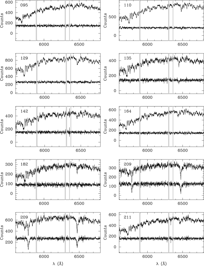
Figure 2.— The galaxy spectra, extracted from an aperture of 5 CCD rows. These spectra are not smoothed. Beneath each spectrum are the residuals from the velocity dispersion fit using template HD72324. The regions of bright sky emission lines around Na I, 6300 [O I] and 6364 [O I] are shown. Note the wide range of Balmer line residuals. Signal-to-Noise estimates are listed in Table 3

Fig.  2. (continued) —

Fig.  2. (continued) —

Fig.  2. (continued) —

Fig.  2. (continued) —

Fig.  2. (continued) —

Figure 3.— The resolution of the May 1996 stellar templates with wavelength, in the frame of CL1358+62. The open circles denote the arc line widths, and the filled circles show the resolution as derived using the solar spectrum. The dotted line shows the fit of a cubic to the filled circles. The resolution determined from the arc lines is similar to that derived using the solar spectrum, and the match is especially good over the range within which the velocity dispersion fitting will be performed, from $\scriptscriptstyle\sim$4200 Å to $\scriptscriptstyle\sim$5100 Å, in the restframe of the galaxies.

Figure 4.— The instrumental resolution of the spectrograph as functions of wavelength for the slitlets of several galaxies in one of the multi-slit masks. The points represent the individual sky line widths for the lines shown in Table 2. The solid line is the low-order polynomial fit to these line widths. The dashed and dotted lines represent the resolution of the stellar templates from May and August, respectively. The vertical dotted lines bracket the wavelength range in which the galaxy kinematics will be derived.

Figure 5.— A histogram of the differences in $\log\sigma$ between the adopted velocity dispersions, $\sigma_{\rm DF,K}$, derived using the fitting method in §5.2, and velocity dispersions derived using a real-fitting variant of the Fourier Fitting method, $\sigma_{\rm DF,F}$. The data used are listed in in Table 3. The median offset is $<1\%$.

Figure 6.— A histogram of the differences in $\log\sigma$ between dispersions derived using the fitting method in §5.2, and velocity dispersions derived using the Fourier Fitting method of Franx et al. (1989). The comparison shown was made using the adopted template HD72324, and uniform pixel weighting. As in Fig. 5, the median offset is $<1\%$. We conclude that velocity dispersion derived using the techniques in §5.2 can be compare directly to measurements made using the Fourier Fitting method on nearby galaxies.

Figure 7.— (a) A comparison of velocity dispersions derived using different template stars. These measurements were made using the direct fitting algorithm outlined in §5.2. The dispersions derived from each template are compared here to the average of the dispersions derived from the five G9-K3 templates. (b) The reduced $\chi^{2}$ of the fit for each template as a function of velocity dispersion. For galaxy #360, $\chi^{2}$ does not vary greatly with template because of poor $S/N$.

Figure 8.— A comparison of $\sigma$ measured from the left and right halves of each spectrum. The difference in dispersions measured from the left and right halves of the galaxy spectra are shown as a function of $\sigma$ for a given template. The direct fitting method of §5.2 was used, with pixel-weighting and masking wherever necessary.

Figure 9.— Spatial profiles of $V$, and $\sigma$. These have not been corrected for seeing effects, or for inclination.

Fig.  9. (continued) —

Fig.  9. (continued) —

Figure 10.— The logarithmic gradient of the second moment of the kinematics, $\mu_{2}=\sqrt{\sigma^{2}+V^{2}}$, of nearby galaxies using long-slit observations from the literature (Simien & Prugniel 1997a ,b,c). A first-order least-squares fit to these data is shown as the solid line. A second order least-squares fit to the rms scatter is used to show the $\pm 1\sigma$ and $\pm 2\sigma$ variation with radius along galaxy major-axis (the dashed lines). The profiles of the CL1358+62 galaxies, shown in Figure 11, are very similar to those shown here of nearby galaxies.

Figure 11.— The logarithmic gradients of the second moment of the kinematics, $\mu_{2}=\sqrt{\sigma^{2}+V^{2}}$ as functions of radius in arcsec (a,c), and radius with respect to the half-light radii of the galaxy (b,d; from bulge-plus-disk profile fitting to HST surface photometry; see Kelson et al. 1999a ). These have not been corrected for seeing effects. Artificial scatter has been added to the radii in (a,c) to aid in displaying the data. The E/S0 galaxies are shown in the top panels, and the spirals in the bottom. Within a half-light radius, the kinematic profiles appear to be independent of morphology. The least-squares fit to the local data of Fig. 10 are shown here in (b,d) and indicate that the kinematic gradients of the CL1358+62 galaxies are similar to nearby galaxies.

Figure 12.— Histogram of measured velocity dispersions.

Figure 13.— (a) $Q$, a quality of fit defined as the ratio of galaxy flux to the standard deviation of the residuals of the velocity dispersion fit, as a function of the expected $S/N$ per pixel. (b) the ratio of $Q/(S/N)$ as a function of $S/N$. Note that the higher the $S/N$, the more the residuals from the velocity dispersion fit become dominated by sources of error other than the expected noise. In (c), we plot the ratio of velocity dispersion to its formal error, $\sigma/\delta_{\sigma}$, as a function of $Q$, and in (d) and (e), we plot the ratio of $\sigma/\delta_{\sigma}$ to $Q$ as functions of $Q$ and $\gamma$, respectively. The formal uncertainties in the velocity dispersions are reasonably well given by the quality of the velocity dispersion fit, though $\gamma$, the line-strength, is clearly a third parameter, indicating that template mismatch is playing a role. The five data points in the lower left corner of (e) are the E+A and emission line galaxies, which are poorly fit by the G9III template star, even when the Balmer lines are excluded from the fit. In these cases, the formal errors of the velocity dispersions are higher than one would expect from the quality of the fit, presumably because of mismatch with the late-type stellar template.

Table 1Stellar Templates

ID	Spectral	Date of
	Type	Observation
The Sun (twilight)	G2V	5/96
HD5268	G5IV	8/96
HD102494	G9IV	5/96
HD6833	G9III	8/96
HD72324a	G9III	5/96
HD56224	K1III	5/96
HD4388	K3III	8/96

Note. — Best-fit template

Table 2Features used to Measure the Instrumental Resolution for the Galaxy Spectra

$\lambda$	Species		$\lambda$	Species
5224.137	9-2 P1(2.5)		6533.044	6-1 P1(2.5)
5238.747	9-2 P1(3.5)		6553.617	6-1 P1(3.5)
5577.338	[O I]		6577.183	6-1 P1(4.5)
5589.128	7-1 P1(2.5)		6596.643	6-1 P2(4.5)
5605.143	7-1 P1(3.5)		6603.990	6-1 P1(5.5)
5915.301	8-2 P1(2.5)		6889.288	7-2 P2(1.5)
5924.723	8-2 P2(2.5)		6900.833	7-2 P1(2.5)
5932.862	8-2 P1(3.5)		6912.623	7-2 P2(2.5)
5953.420	8-2 P1(4.5)		6923.220	7-2 P1(3.5)
5970.278	8-2 P2(4.5)		6939.521	7-2 P2(3.5)
6192.937	5-0 P2(1.5)		6948.936	7-2 P1(4.5)
6202.720	5-0 P1(2.5)		6969.930	7-2 P2(4.5)
6221.771	5-0 P1(3.5)		6978.258	7-2 P1(5.5)
6287.434	9-3 P1(2.5)		7003.858	7-2 P2(5.5)
6300.304	[O I]		7011.202	7-2 P1(6.5)
6363.780	[O I]

Note. — Wavelengths and identifications taken from Osterbrock et al. (1997).

Table 3Final Velocity Dispersions

							Adopted
ID	Morphology	$S/N$ per Å		$\sigma_{\rm DF,F}$b (km/s)			$\sigma_{\rm DF,K}$b (km/s)
95	S0	48		219.1	$\pm 6.4$		220.5	$\pm 6.4$
110	S0/a	71		171.8	3.7		174.8	3.7
129	S0/a	65		167.0	3.6		167.5	3.8
135	S0	40		161.2	5.4		159.7	5.1
142	S0/a	43		148.4	4.5		147.9	4.4
164	S0/a	51		181.0	4.5		180.6	4.3
182	S0	28		132.5	5.6		130.1	5.4
209a	Sa	35		66.3	7.7		73.5	7.5
209a	Sa	63		109.0	5.8		107.9	5.2
211	S0	44		189.1	6.2		190.5	6.4
212	E	53		182.3	4.9		181.0	5.7
215	S0	33		162.7	6.1		166.2	5.9
233	E/S0	74		238.0	4.3		234.9	4.5
234	Sb	42		113.1	8.5		108.9	8.2
236	S0	43		197.9	5.7		196.7	5.6
242	E	58		207.6	5.2		212.4	5.3
256	E	93		257.8	4.1		261.8	4.3
269	E/S0	92		317.2	5.4		319.5	5.8
283	Un	34		147.2	5.2		145.7	5.2
292	S0	56		111.3	3.5		112.3	3.2
298	S0	85		296.1	5.5		296.6	5.2
300	S0	60		254.4	5.7		248.2	5.5
303	E	52		164.5	4.0		163.5	4.3
309	E/S0	61		229.9	4.7		228.7	4.7
328	Sa	59		75.8	4.7		81.2	4.2
335	S0/a	37		128.0	4.6		129.1	4.3
343	S0	36		63.1	5.6		65.1	5.0
353	E/S0	77		223.6	4.3		228.5	4.4
356	Sa	64		191.5	3.8		190.2	3.7
359	S0	56		198.7	4.4		200.3	4.5
360	E	9		173.7	17.7		177.5	19.7
366	S0/a	43		226.3	6.6		228.9	6.4
368	Sab	21		148.2	7.4		145.6	7.5
369	S0/a	36		129.7	6.3		128.2	6.1
371	Sa	59		175.9	3.9		174.8	4.0
372	Sa	45		144.7	5.0		142.3	5.0
375	E	78		307.0	6.9		311.3	7.0
381	E/S0	48		210.6	5.6		212.4	5.5
391	E/S0	62		252.9	7.1		260.1	6.3
397	S0/a	38		135.1	5.2		135.9	5.1
408	S0	47		233.3	6.2		237.1	6.2
409	E	21		106.9	6.9		107.3	6.7
410	S0	32		150.9	5.0		148.6	5.2
412	E	41		170.7	6.3		169.4	6.3
433	S0/a	37		104.4	3.7		106.6	4.0
440	S0/a	25		61.0	4.8		63.7	5.0
454	S0/a	63		149.1	3.8		149.6	3.7
463	S0	57		284.6	6.4		284.4	6.4
465	Sa	37		156.3	4.7		156.7	5.0
481	S0	25		106.8	6.0		107.2	5.5
493a	E/S0	18		118.7	9.0		116.5	8.3
493a	E/S0	17		125.1	10.1		127.5	8.8
523	S0/a	42		171.8	5.9		174.6	5.9
531	E	90		285.3	4.8		281.3	5.0
534	E	30		120.3	6.2		120.9	6.1
536	E	72		252.2	5.0		254.1	5.0
549	Sab	30		79.9	4.7		79.9	4.6

Note. — Notes: $\sigma_{\rm DF,F}$ refers to measurements made using an analog of the Fourier Fitting method except that the $\chi^{2}$ summation is performed in the real domain. $\sigma_{\rm DF,K}$ refers to measurements made using the direct fitting method of §5.2. (a) Galaxies #209 and #493 were observed in two different slit-masks and position angles. The first listed value for #209 was derived from a mis-aligned slitlet (see §9.5). (b) These values have been corrected for aperture size to a nominal aperture with diameter of 3^′′.4 at the distance of Coma.

References

- Bender (1990) Bender, R. 1990, A&A, 229, 441
- Bender et al. (1994) Bender, R., Saglia, R.P., & Gerhard, O.E. 1994, MNRAS, 269, 785
- Bender et al. (1998) Bender, R., Saglia, R.P., Ziegler, B., Belloni, P., Greggio, L., & Hopp, U. 1998, ApJ, 493, 529
- Binney & Tremaine (1987) Binney, J. & Tremaine, S. 1987, Galactic Dynamics, (Princeton: Princeton University Press)
- Butcher & Oemler (1978) Butcher, H. & Oemler, A., Jr. 1978, ApJ, 219, 18
- Caldwell & Rose (1997) Caldwell, N., & Rose, J. 1997, AJ, 113, 492
- Caldwell & Rose (1998) Caldwell, N., & Rose, J. 1998, AJ, 115, 1423
- Ciotti, Lanzoni, & Renzini (1996) Ciotti, L., Lanzoni, B., & Renzini, A. 1996, MNRAS, 282, 1
- Davies et al. (1983) Davies, R.L., Efstathiou, G., Fall, S.M., Illingworth, G.D., & Schechter, P.L. 1983, ApJ, 266, 41
- Davies & Illingworth (1983) Davies, R.L. & Illingworth, G.D. 1983, ApJ, 256, 516
- Djorgovski & Davis (1987) Djorgovski S., & Davis M. 1987, ApJ, 313, 59
- Dressler (1980) Dressler, A. 1980, ApJ, 236, 351
- Dressler & Gunn (1983) Dressler A., & Gunn J. E. 1983, ApJ, 270, 7
- Dressler et al. (1997) Dressler, A., Oemler, A., Jr., Couch, W. J., Smail, I., Ellis, R. S., Barger, A., Butcher, H., Poggianti, B. M., & Sharples, R. M. 1997, ApJ, 490, 577
- Ellis et al. (1997) Ellis R. S., Smail, I., Dressler, A., Couch, W.J., Oemler, A., Jr., Butcher, H., & Sharples, R.M. 1997, ApJ, 483, 582
- Faber et al. (1987) Faber S. M., Dressler A., Davies R. L., Burstein D., Lynden-Bell D., Terlevich R., & Wegner G. 1987, Faber S. M., ed., Nearly Normal Galaxies. Springer, New York, p. 175
- Fabricant, McClintock, & Bautz (1991) Fabricant, D.G., McClintock, J.E. & Bautz, M.W. 1991, ApJ, 381, 33
- Fabricant et al. (1999) Fabricant, D.G., et al. 1999, in preparation
- Fisher (1997) Fisher, D. 1997, AJ, 113, 950
- Fisher et al. (1998) Fisher, D., Fabricant, D.G., Franx, M., & van Dokkum P.G. 1998, ApJ, 498, 195
- Franx (1993) Franx M. 1993, PASP, 105, 1058
- Franx (1995) Franx, M. 1995, IAU Symposium 164, “Stellar Populations” ed. P.C. van der Kruit & G. Gilmore (Dordrecht:Kluwer), 269
- Franx & Illingworth (1988) Franx M., & Illingworth, G.D. 1988, ApJL, L55
- Franx, Illingworth, & Heckman (1989) Franx, M., Illingworth, G.D. & Heckman, T. 1989, AJ, 98, 538
- Franx et al. (1997) Franx M., et al. 1997, in preparation
- (26) Gillingham, P. 1996, private communication
- Gioia et al. (1992) Gioia, I. M., Maccacaro, T., Schild, R. E., Wolter, A., Stocke, J. T., Morris, S. L., Henry, J. P. 1990, ApJS, 72, 567
- González (1993) González, J.J. 1993, Ph.D. thesis, Univ. Calif., Santa Cruz
- Jørgensen et al. (1993) Jørgensen I., Franx M., & Kjærgaard P. 1993, ApJ, 411, 34
- Jørgensen et al. (1995) Jørgensen I., Franx M., & Kjærgaard P. 1995, MNRAS, 276, 1341
- Jørgensen et al. (1996) Jørgensen I., Franx M., & Kjærgaard P. 1996, MNRAS, 280, 167 [JFK96]
- Kelson et al. (1997) Kelson, D.D., van Dokkum, P.G., Franx, M., Illingworth, G.D., & Fabricant, D.G. 1997, ApJL, 478, L13
- Kelson (1998) Kelson, D.D. 1998, Ph.D. thesis, Univ. Calif., Santa Cruz
- (34) Kelson, D.D., Illingworth, G.D., van Dokkum, P.G., & Franx, M. 1999a, ApJ, in preparation
- (35) Kelson, D.D., Illingworth, G.D., van Dokkum, P.G., & Franx, M. 1999b, ApJ, in preparation
- (36) Kelson, D.D., et al. 1999c, ApJ, in preparation
- (37) Kelson, D.D., Trager, S.C., Zabludoff, A., Bolte, M., & Mulchaey, J. 1999d, ApJL, in preparation
- Luck & Challener (1995) Luck, R.E. & Challener, S.L. 1995, AJ, 100, 2968
- Oke et al. (1995) Oke, J.B., et al. 1995, PASP, 107, 375
- Osterbrock et al. (1996) Osterbrock, D.E., Fulbright, J.P., Martel, A.R., Keane, M.J., Trager, S.C., & Basri, G. 1996, PASP, 108, 2770
- Pahre (1998) Pahre, M.A., 1998, Ph.D. thesis, California Inst. of Technology
- Pilachowski, Sneden, & Kraft (1996) Pilachowski, C.A., Sneden, C. & Kraft R.P. 1996, AJ, 111, 1689
- Prugniel & Simien (1996) Prugniel, Ph. & Simien, F. 1996, A&A, 309, 749
- Rix & White (1992) Rix, H.-W. & White, S.D.M. 1992, MNRAS, 254, 389
- Schade et al. (1997) Schade, D., Carlberg, R.G., Yee, H.K.C & López-Cruz, O. 1997, ApJL, 477, L17
- (46) Simien, F., Prugniel, P. 1997a, A&AS, 122, 521
- (47) Simien, F., Prugniel, P. 1997b, A&AS, 126, 15
- (48) Simien, F., Prugniel, P. 1997c, A&AS, 126, 519
- Simkin (1974) Simkin, S.M. 1974, A&A, 31, 129
- Terlevich et al. (1981) Terlevich, R.J., Davies, R.L., Faber, S.M. & Burstein, D. 1981, MNRAS, 196, 381
- Tonry (1983) Tonry, J. 1983, ApJ, 266, 58
- Tully & Fisher (1977) Tully, R.B. & Fisher J.R. 1977, A&A, 54, 661
- van Dokkum & Franx (1996) van Dokkum, P. G., & Franx M. 1996, MNRAS, 281, 985
- (54) van Dokkum, P.G., Franx, M., Illingworth, G. D., Kelson, D. D., Fisher, D., & Fabricant, D. 1998a, ApJ, 500, 714
- (55) van Dokkum, P. G., Franx, M., Kelson, D.D., & Illingworth, G.D. 1998b, ApJ, 504, L17
- Vogt et al. (1996) Vogt, N. P., Forbes, D. A., Phillips, A. C., Gronwall, C., Faber, S. M., Illingworth, G. D., & Koo, D. C. 1996, ApJL, 465, L15
- Vogt et al. (1997) Vogt, N. P., Phillips, A. C., Faber, S. M., Gallego, J., Gronwall, C., Guzmán, R., Illingworth, G. D., Koo, D. C., & Lowenthal, J.D. 1997, ApJL, 479, L121
- Wirth, Koo, & Kron (1994) Wirth, G.D., Koo, D.C., & Kron, R.G. 1994, ApJL, 435, L105
- Ziegler & Bender (1997) Ziegler, B. L., & Bender, R. 1997, MNRAS, 291, 527