SIZE OF THE VELA PULSAR’S EMISSION REGION AT 13 cm WAVELENGTH

Abstract

We present measurements of the size of the Vela pulsar in 3 gates across the pulse, from observations of the distribution of intensity. We calculate the effects on this distribution of noise in the observing system, and measure and remove it using observations of a strong continuum source. We also calculate and remove the expected effects of averaging in time and frequency. We find that effects of variations in pulsar flux density and instrumental gain, self-noise, and one-bit digitization are undetectably small. Effects of normalization of the correlation are detectable, but do not affect the fitted size. The size of the pulsar declines from $440\pm 90$ km (FWHM of best-fitting Gaussian distribution) to less than 200 km across the pulse. We discuss implications of this size for theories of pulsar emission.

¹ Physics Department, University of California, Santa Barbara, California, 93106, USA

² School of Physics, University of Melbourne, Parkville 3052, Victoria, Australia

³ Australia Telescope National Facility, Epping, New South Wales, 2121, Australia

⁴ Physics Department, University of Tasmania, Hobart, 7001, Tasmania, Australia

⁵ Institute of Space and Astronautical Science, 3-1-1 Yoshinodai, Sagamihara, Kanagawa 229, Japan

⁶ Hartebeesthoek Radio Astronomy Observatory, Krugersdorp, Transvaal, South Africa

⁷ Jet Propulsion Laboratory, California Institute of Technology, Pasadena, California, 91109, USA

1 Introduction

1.1 Pulsar Radio Emission

Pulsars emit meter- to centimeter-wavelength radiation with brightness temperatures of $T>10^{23}$ K, greater than any other astrophysical sources. The ultimate energy source for pulsar emission is rotation of the neutron star. Combined with this rotation, the neutron star’s magnetic field generates forces sufficient to accelerate electrons from the stellar surface. These energetic electrons or the gamma-rays they emit can pair-produce after a few centimeters. The consequent cascade of electron-positron pairs permeates the magnetic field of the pulsar out to the light cylinder. The electrons and positrons follow the lines of the strong magnetic field closely. Particles on the “open” field lines, which pass through the light cylinder, gradually carry away part or all of the rotational kinetic energy of the pulsar as an electron-positron wind, leading to the observed spindown of the pulsar. The “polar cap” is the region defined by the open field lines at the surface of the neutron star, from which the wind is drawn. This basic picture has long been understood (Goldreich & Julian (1969), Sturrock (1971), Ruderman & Sutherland (1975), Arons (1983)). Despite this understanding, the physical mechanism for conversion of a small fraction of the spindown power to a beam of radio emission, which sweeps past the observer each rotation period to produce the observed pulses, remains uncertain. Observational tests of models for pulsar emission are difficult because the emission is so compact. It cannot be resolved with instruments of Earthlike or smaller dimensions.

Melrose (1996) and Asseo (1996) recently reviewed theories of pulsar emission. In all models, collective behavior of the electron-positron plasma results in coherent emission from groups of particles. Melrose divides theories into 4 categories, according to location of the emission region: (i) at a pair-production front at the polar cap; (ii) in the electron-positron wind on open field lines above the polar cap; (iii) in the electron-positron wind far above the cap, near the light cylinder; and (iv) at, or even outside, the light cylinder. Theories from all 4 categories appear viable. Indeed, more than one emission mechanism may act, to produce the wide range of observed pulse morphologies (Rankin (1983)).

Pulsars exhibit rich temporal structure, including complicated variations of structure of individual pulses about an average, and large pulse-to-pulse variations in flux density; these offer clues to the emission process (Hankins (1972), Lyne & Graham-Smith (1998)). Because the fundamental modes of lower-frequency electromagnetic waves are linearly polarized, either across or along the pulsar’s magnetic field (Blandford & Scharlemann (1976), Melrose & Stoneham (1977), Arons & Barnard (1986), Lyutikov 1998a ), the strong linear polarizations of pulsars yield the direction of the pulsar’s magnetic field at the locus of emission (Radhakrishnan & Cooke (1969)). Polarization observations usually suggest that emission arises near the magnetic pole of the neutron star, which is offset from the rotation pole.

Pulsars show stable, sometimes complicated long-term average profiles, but with large pulse-to-pulse variations. The most successful classification of these profiles is that of Rankin (Rankin (1983), Rankin (1990)), who divides emission into “core” and “cone” components, corresponding respectively to elliptical pencil beams and hollow cones directed from above the magnetic pole of the neutron star. A host of associated pulse properties support this classification (Rankin (1986), Lyne & Manchester (1988), Radhakrishnan & Rankin (1990)). The existence of these different components may indicate the presence of more than one emission process (Lyne & Manchester (1988), Weatherall & Eilek (1997)). A few core emitters show interpulses, suggesting that their magnetic poles lie near the rotation equator. Comparison of pulse width with period for these pulsars, and extension of this relation to all core emitters, closely tracks the relation expected if the size of the polar cap sets the angular width of the beam for core emission (Rankin (1990)). Rankin concludes that core emission arises very near the surface of the neutron star.

Interstellar scattering offers the possibility of measuring the sizes of pulsars and the structure of the emission region, and its changes over the pulse, using effective instruments of AU dimensions (Backer (1975), Cordes, Weisberg & Boriakoff (1983), Wolszczan & Cordes (1987), Smirnova et al. (1996), Gwinn et al. (1997), Gwinn et al. (1998)). In this paper, we describe measurement of the size of the Vela pulsar, from the distribution of flux density in interstellar scintillation, observed on a short interferometer baseline.

1.2 Interstellar Scattering

Density fluctuations in the interstellar plasma scatter radio waves from astrophysical sources. These fluctuations act as a corrupt lens, with typical aperture of about 1 AU. Like such a lens, scattering forms a diffraction pattern in the plane of the observer. For a spatially-incoherent source, the intensity of the pattern is the convolution of the intensity of the pattern for a point source, with an image of the source (Goodman 1968). The scattering system has resolution corresponding to the diffraction-limited resolution of the “scattering disk”, the region from which the observer receives radiation.

The finite size of the scattering disk sets a minimum spatial scale for the diffraction pattern in the plane of the observer, at the diffraction limit. This scale is $\lambda/\theta$, where $\lambda$ is the observing wavelength and $\theta$ is the angular standard deviation of the scattering disk, as seen by the observer. If the plasma fluctuations are assumed to remain “frozen” in the medium, while the motions of pulsar, observer, and medium carry the line of sight through it at speed $V_{\perp}$, this spatial scale sets the timescale of scintillations, $t_{ISS}=\lambda/\theta V_{\perp}$. Differences in travel time from the different parts of the scattering disk set the minimum frequency scale of the pattern, at $\Delta\nu={{c}\over{2\pi}}(\theta D)^{-2}{\left[{{1}\over{D}}+{{1}\over{R}}\right]^{-1}}$, where $D$ is the characteristic distance from observer to scatterer, and $R$ is the characteristic distance from scatterer to source. Observations with time resolution shorter than $t_{ISS}$ and with frequency resolution finer than $\Delta\nu$ are in the “speckle limit” of interstellar scattering.

For an extended, spatially-incoherent source, overlap of different parts of the image of the source in the observer plane, after the convolution, reduces the depth of modulation of scintillation: “stars twinkle, planets do not.” The relation of Cohen et al. (1967) and Salpeter (1967) quantifies this fact as a relation between the size of the source and the depth of modulation of scintillations.

1.3 The Vela Pulsar

The Vela pulsar is particularly well-suited for studies of pulsar emission because it is strong, heavily scattered, and relatively nearby. In a typical “scintle” of observing time $t_{ISS}$ and bandwidth $\Delta\nu$, a typical terrestrial radiotelescope can attain a signal-to-noise ratio of a few, for observations of the Vela pulsar at decimeter wavelengths. A short observation can thus sample many scintles. Moreover, the scattering disk is large enough at these wavelengths that the scale of the diffraction pattern is on the order of the size of the Earth, so that different radiotelescopes on Earth can sample different scintles. The nominal linear resolution of the scattering disk, acting as a lens, is about 1000 km at the pulsar. For the Vela pulsar, the diameter of the light cylinder is 8500 km. In contrast, the size of the polar cap is tens of meters, for a dipole magnetic field and a $\sim 10$ km radius for the neutron star. Thus, observations of the scintillation pattern can distinguish among different theories of pulsar emission, as discussed in §1.1.

Among the properties that place the Vela pulsar’s pulse into the core class are its single component, varying little in width with frequency; its short period and rapid spindown rate; its circular polarization; and its weak, irregular pulse-to-pulse variations (Rankin (1983), Rankin (1990)). However, Vela also shows characteristics of cone emission, including strong, well-ordered linear polarization and a double profile in X- and gamma rays (Strickman et al. (1996)). Indeed, Radhakrishnan et al. (1969) first observed in the Vela pulsar the S-shaped variation of the direction of linear polarization characteristic of cone pulsars. Manchester (Manchester (1995)) has proposed that Vela’s pulse (and those of some other young pulsars) could represent one side of broad cone, which would help to explain the apparent inconsistency. On the other hand, Romani & Yadigaroglu (1995) propose that the radio pulse is indeed core emission, perhaps from very close to the polar cap, and that the double-peaked X- and gamma-ray emission arises far out in the magnetosphere, near the light cylinder.

Krishnamohan & Downes (1983) performed an extensive study of 87040 pulses from the Vela pulsar, and found that the pulse shape varied with peak intensity. Notably, strong pulses tend to arrive earlier. They also found that the rate of change of angle of linear polarization changes with pulse strength, and interpreted this as activity from emission regions at different altitudes and magnetic longitudes. They inferred variations in the location of the emission region by about 400 km in altitude, and by about about $4^{\circ}$ in longitude. Emission earlier in the pulse was found to arise further from the star, and from a larger region.

2 Distribution of Interferometric Correlation

Interferometers present several advantages over single antennas for observations of scintillating sources. Because noise does not correlate between antennas, no baseline response need be subtracted from observations. Moreover, interferometers are nearly immune to interference and emission from extended or unrelated nearby sources. The statistics of interferometer response to signals and noise is well studied (see, for example, Thompson, Moran, & Swenson (1986)). For a short interferometer baseline, interferometers measure the intensity of the source, commonly expressed as flux density. Disadvantages of interferometers include the facts that they require coordinated observations at multiple antennas, and so often yield smaller effective apertures than the largest available single antenna; and they often afford narrower bandwidths than some observing modes at single antennas. For the present work, careful treatment of statistics is essential and interferometers are preferred. We focus on observations of scintillating sources on short interferometric baselines in this paper.

2.1 Distribution of Flux Density for a Small Source

For a point source in strong scintillation, sampled in the speckle limit, the distribution of flux density follows an exponential distribution (Scheuer (1968), Goodman (1985)):

$$P(S)=1/S_{0}\,\exp\{-S/S_{0}\}.$$ (1)

This equation holds if the source is small, compared with the resolution of the scattering disk treated as a lens, so that $kM\theta\sigma_{s}<<1$, where $M=D/R$ is the magnification of that lens, and $k=2\pi/\lambda$ where $\lambda$ is the observing wavelength. The size of the source, parametrized as the standard deviation of a circular Gaussian distribution of intensity, is $\sigma_{s}$. If $kM\theta\sigma$ is finite but small compared with 1, then the distribution of flux density is the weighted sum of 3 exponentials (Gwinn et al. (1998)). If, for example, the scattering disk is modeled as an elliptical Gaussian, and the source is modeled as a circular Gaussian, then the exponential scales are

$$S_{0},\quad S_{1\xi}=S_{0}(kM\theta_{\xi}\sigma_{s})^{2},\quad{\rm and}\quad S_{1\eta}=S_{0}(kM\theta_{\eta}\sigma_{s})^{2},$$ (2)

where $\theta_{\xi}$ and $\theta_{\eta}$ are the angular standard deviations of the scattering disk along the major and minor axes, and $S_{0}$ sets the scale of flux density. We assume that $(kM\theta\sigma_{s})<<1$; this is equivalent to the assertion that the scattering disk, treated as a lens, does not resolve the source. The probability distribution for flux density is then:

$$P(S) = {\textstyle{{S_{0}}\over{(S_{0}-S_{1\xi})(S_{0}-S_{1\eta})}}\exp{\left\{-S/S_{0}\right\}}+{{S_{1\xi}}\over{(S_{1\xi}-S_{0})(S_{1\xi}-S_{1\eta})}}\exp{\left\{-S/S_{1\xi}\right\}}}$$

$${\textstyle\quad+{{S_{1\eta}}\over{(S_{1\eta}-S_{1\xi})(S_{1\eta}-S_{0})}}\exp{\left\{-S/S_{1\eta}\right\}}.}$$

At large flux denisty, the first term dominates and the distribution remains exponential, but with different scale $S_{0}$ and normalization than for a point source. At small flux density, the probability density falls to zero at zero flux density, in a way that depends on source size $\sigma_{s}$. The larger the source, the more sharply the distribution of flux density is peaked near the average flux density. Figure 1 shows sample distributions. In this paper, we use this expression, with modifications for the effects of noise, to find the size of the Vela pulsar in 3 gates across the pulse.

Source size reduces the intensity variation due to scintillation. The Cohen-Salpeter relation formalizes this fact as a relation between angular size and modulation index, $m=\sqrt{\langle I^{2}\rangle-\langle I\rangle^{2}}/\langle I\rangle$. Here the angular brackets $\langle...\rangle$ denote an ensemble average, approximated in practice by a time average. For a circular Gaussian source viewed through a elliptical scattering disk, in strong scattering (Gwinn et al. (1998)),

$$m^{2}=(1+(2kM\theta_{\eta}\sigma_{s})^{2})^{-1/2}(1+(2kM\theta_{\eta}\sigma_{s})^{2})^{-1/2}.$$ (4)

This expression is valid for arbitrarily large source size $\sigma_{s}$. The modulation index calculated from Eq. 2.1 is consistent with this expression in the limit $kM\theta_{\eta}\sigma_{s}<<1$.

2.2 Effects of Averaging in Time and Frequency

Because the scintillation pattern varies with time and frequency, integration over either reduces the depth of modulation and narrows the distribution of amplitude. It thus affects the distribution in a way similar to finite source size. Averaging leaves the mean flux density $\langle S\rangle$ unchanged, but reduces the mean square flux density $\langle S^{2}\rangle$, and so reduces the modulation index. We can calculate the effects of averaging on the modulation index, and liken them to the effects of source size, to assess effects of averaging on estimates of source size.

For a source with pointlike or Gaussian intensity distribution, seen through a Gaussian scattering disk, the correlation flunction of flux density with frequency follows a Lorentzian distribution (see, for example, Gwinn et al. (1998)):

$$\langle S(\nu)S(\nu+d\nu)\rangle=\langle S(\nu)^{2}\rangle\left({{1}\over{1+(d\nu/\Delta\nu)^{2}}}+1\right),$$ (5)

where $\nu$ and $\nu+d\nu$ are the observing frequencies, and $\Delta\nu$ is the decorrelation bandwidth of the scintillations. For a small source with a Gaussian distribution of intensity, the correlation function has the same form, with larger decorrelation bandwidth. For non-Gaussian spectra of density fluctuations in the scattering material, the correlation function shows the same behavior, with a different functional form (Codona et al. (1986)). After averaging in frequency by convolving with a “boxcar” of bandwidth $B$, the mean intensity is unchanged, and the mean square intensity becomes

$$\langle\bar{S}(\nu)^{2}\rangle = \langle{{1}\over{B^{2}}}\int_{0}^{B}dx\,\int_{0}^{B}dy\,S(\nu+x)S(\nu+y)\rangle$$

$$= {{2}\over{B}}\int_{0}^{B}du\,(B-u)\langle S(\nu)S(\nu+u)\rangle$$

$$= \langle S(\nu)^{2}\rangle\left[{{\tan^{-1}(B/\Delta\nu)}\over{B/\Delta\nu}}+{{1}\over{2}}-{{\ln(1+(B/\Delta\nu)^{2})}\over{2(B/\Delta\nu)^{2}}}\right].$$

$$\equiv \langle S(\nu)^{2}\rangle f_{f}$$

Here the bar on $\bar{S}$ denotes averaging. This expression defines the convenient factor $f_{f}$.

A similar approach yields effects of averaging in time. The spatial scintillation pattern for a point source is the Fourier transform of the screen phase (Goodman (1985), Cornwell et al. (1989) Gwinn et al. (1998)). Commonly, it is assumed that scintillation in time represents the motion of the scintillation pattern across the instrument, while the screen and pattern remain unchanged. For an extended source, the pattern is the convolution of the point-source response with an image of the source. If both source and scattering disk follow Gaussian distributions of intensity, then the correlation function in time is Gaussian:

$$\langle S(t)S(t+dt)\rangle=\langle S(t)^{2}\rangle\exp\left\{-\ln(2)(dt/t_{ISS})^{2}\right\},$$ (7)

where $t$ and $t+dt$ are the times of observation, and $t_{ISS}$ is the timescale of interstellar scintillation. If the observer averages over time interval $\tau$, the mean square flux density after that averaging is

$$\langle{\bar{S}}^{2}\rangle=\langle S^{2}\rangle\left[{\textstyle{{1}\over{\alpha}}}\sqrt{\pi}\,{\rm erf}(\alpha)+{\textstyle{{1}\over{\alpha^{2}}}}e^{-\alpha^{2}}-{\textstyle{{1}\over{\alpha^{2}}}}\right]\equiv\langle S^{2}\rangle f_{t}$$ (8)

where $\alpha=\sqrt{\ln 2}\;\tau/t_{ISS}$.

The effects of averaging can be expressed as a reduction in modulation index or an increase in inferred source size. The post-averaging modulation index $\bar{m}$ is related to the pre-averaging value by

$$\bar{m}^{2}=f_{f}f_{t}(m^{2}+1)-1.$$ (9)

Using Eq. 4 we can infer a post-averaging size $\bar{\sigma}_{s}$ from $\bar{m}$, and so relate $\bar{\sigma}_{s}$ to the true size $\sigma_{s}$, using knowledge of the averaging bandwidth and time. This is the approach taken below.

2.3 Noise and Self-Noise for Scintillating Sources

The effects of noise can be important for studies of scintillating pulsars because the scintles of lowest flux density are important in determining the size of the source. Similarly, noise affects the distribution of intensity most strongly at the lowest intensities. Thus, noise is important in determining source size.

2.3.1 Noise and Self-Noise for Interferometric Correlation

The interferometrist observes the signal from the source, along with noise, at 2 stations $1$ and $2$ and measures their correlation: ${{\bf C}_{12}}=C_{x}+iC_{y}={{1}\over{N_{q}}}\sum_{p=1}^{N_{q}}({\bf V}_{1p}{\bf V}_{2p}^{*})$. The correlation ${{\bf C}_{12}}$ is often called the interferometric visibility, and is often expressed in units of flux density, using the measured or estimated gains of the antennas. For interferometric observations, ${{\bf C}_{12}}$ is complex (Thompson, Moran, & Swenson (1986)). In this paper, we use boldface characters to denote complex quantities. Here ${\bf V}_{1,2}$ are the electric fields in the observed polarization, at the two antennas; and $N_{q}$ is the number of independent samples, the product of integration time and bandwidth. System noise may be in or out of phase with the signal, and so contributes to both real and imaginary components. Signals from astrophysical sources are intrinsically noiselike, and their stochastic variations represent another source of noise, known as self-noise. Self-noise contributes only in phase with the signal. Without loss of generality, we take the phase of the signal to define the real axis. Self-noise then affects only the real component.

For a strongly-scintillating point source, the measured correlation ${{\bf C}_{12}}$ is drawn from the distribution:

$$P({\bf C}_{12})=\int du{{1}\over{2\pi\sigma^{2}}}\exp\left\{-{{1}\over{2}}{{(C_{x}-u)^{2}+C_{y}^{2}}\over{\sigma^{2}}}\right\}\;\int dS\,f(u/S;N_{q})\;{{1}\over{S_{0}}}\exp\left\{-{{S}\over{S_{0}}}\right\},$$ (10)

where $f(u/S;N_{q})$ is the chi-square distribution with $N_{q}$ degrees of freedom (see, for example, Meyer (1975)). Again, $S_{0}$ is the mean flux density of the source, averaged over many scintles. We measure the correlation in units of flux density, using the gains of the antennas $\Gamma_{1,2}$. The system noise in units of flux density is $\sigma^{2}=(T_{S1}/\Gamma_{1})(T_{S2}/\Gamma_{2})/N_{q}$ where $T_{S1,2}$ are the system temperatures at stations 1 and 2, and $\Gamma_{1,2}$ are the gains at stations 1 and 2. This equation assumes that the noise from the source has Gaussian statistics. In practice the radiation from all known astrophysical sources does appear to have Gaussian statistics. In particular, radiation from pulsars follows Gaussian statistics closely, with time-varying amplitude (Rickett (1975)). For some pulsars, the amplitude varies quite dramatically over short times within the pulse (Hankins (1972), Lyne & Graham-Smith (1998)), although the Vela pulsar seems to be relatively stable in this respect.

When the number of independent samples $N_{q}$ is large, the chi-squared distribution is well approximated by a Gaussian, and the distribution takes the form:

$$P({\bf C}_{12})=\int_{0}^{+\infty}dS{{1}\over{2\pi\sigma_{x}}}\exp\left\{-{{{1}\over{2}}}{{(C_{x}-S)^{2}}\over{\sigma_{x}^{2}}}\right\}{{1}\over{2\pi\sigma_{y}}}\exp\left\{-{{{1}\over{2}}}{{C_{y}^{2}}\over{\sigma_{y}^{2}}}\right\}\;{{1}\over{S_{0}}}\exp\left\{-{{S}\over{S_{0}}}\right\}.$$ (11)

The variances of the real and imaginary parts of the correlation are

$$\sigma_{x}^{2}={{{1}\over{N_{q}}}}{(T_{S1}/\Gamma_{1}+S)(T_{S2}/\Gamma_{2}+S)}$$ (12)

and

$$\sigma_{y}^{2}={{{1}\over{N_{q}}}}{(T_{S1}/\Gamma_{1})(T_{S2}/\Gamma_{2})}.$$ (13)

The flux density of the source, $S$, appears in the denominator of the exponent in Eq. 11, through $\sigma_{x}$. This reflects self-noise.

For 2 identical antennas, system temperature and gain are equal, so that $T_{S1}=T_{S2}$ and $\Gamma_{1}=\Gamma_{2}$, and the correlation ${\bf C}_{12}=C_{x}+iC_{y}$ is drawn from the distribution:

$$P({\bf C}_{12}) = {{N_{q}}\over{2\pi S_{0}(T_{S}/\Gamma)}}\exp\left\{-{{(C_{y})^{2}}\over{2(T_{S}/\Gamma)^{2}/N_{q}}}\right\}$$

$$\times\int_{0}^{+\infty}dS{{1}\over{(T_{S}/\Gamma+S)}}\exp\left\{-{{(C_{x}-S)^{2}}\over{2(T_{S}/\Gamma+S)^{2}/N_{q}}}\right\}\exp\left\{-S/S_{0}\right\}.$$

Unfortunately, this integral is not easily simplified. Figure 2 shows plots of the distribution of the amplitude of the correlation, $P(|{\bf C_{12}}|)$, for a scintillating point source, for sample values of $\Gamma S_{0}/T_{S}$ and $N_{q}$. When $N_{q}$ is large, self-noise is negligible and the ratio $S_{0}\Gamma(N_{q})^{1/2}/T_{S}$ is the average signal-to-noise ratio. When $N_{q}$ is small, self-noise becomes important. As the figure shows, self-noise increases the number of points at low amplitude, and flattens the distribution at high amplitude.

2.3.2 Distribution for a Point Source with Noise

If the number of independent samples $N_{q}$ is large, then self-noise can be ignored. The distribution of amplitude, $C_{12}=|{\bf C}_{12}|$, then takes the often-useful form:

$$P_{S}(C_{12},S_{0},\sigma) = P(u)\times{{du}\over{dC_{12}}}$$

$$= {{1}\over{\sqrt{\pi}}}{{1}\over{S_{0}}}\exp({\textstyle{{1}\over{4}}}\beta^{2})\,u$$

$$\quad\times\int_{0}^{\pi}\,d\phi\exp\{-u^{2}\sin^{2}\phi-\beta u\cos\phi\}\left(1+{\rm erf}(u\cos\phi-{\textstyle{{1}\over{2}}}\beta)\right)\times{{1}\over{\sqrt{2}\sigma}},$$

where ${\rm erf}(~{})$ is the error function (Meyer (1975)). The noise, in flux density units, is $\sigma\equiv\sigma_{x}=\sigma_{y}=(T_{S}/\Gamma)$. We have adopted the scaled parameters

$$u=C_{12}/\sqrt{2}\sigma\quad{\rm and}\quad\beta=\sqrt{2}\sigma/S_{0}.$$ (16)

If the antennas are not identical, the distribution has the same form in this limit, but the definitions of the scaled parameters are slightly different. Because self-noise can often be ignored, as Figure 2 suggests, this expression is often appropriate. For scintles much stronger than noise ($C_{12}>>\sigma$), and average flux density not much smaller than noise (so that $S_{0}>>\sigma^{2}/C_{12}$), this distribution approaches the purely-exponential form

$$P(C_{12})\approx\left\{\exp\left({{\sigma^{2}}\over{2S_{0}^{2}}}\right)\right\}{{1}\over{S_{0}}}e^{-C_{12}/S_{0}}.$$ (17)

The constant of the exponential is the same as that for a noise-free scintillating point source, but the normalization is different. In effect, noise shifts the distribution toward greater amplitude.

2.3.3 Distribution for a Small Source with Noise

When the source has small but finite size, and self-noise can be ignored, the distribution of $C_{12}$ takes the form suggested by the combination of Eqs. 2.1 and 2.3.2:

$$P(C_{12}) = {\textstyle{{S_{0}}\over{(S_{0}-S_{1\xi})(S_{0}-S_{1\eta})}}P_{S}(C_{12},S_{0},\sigma)+{{S_{1\xi}}\over{(S_{1\xi}-S_{0})(S_{1\xi}-S_{1\eta})}}P_{S}(C_{12},S_{1\xi},\sigma)}$$

$${\textstyle\quad+{{S_{1\eta}}\over{(S_{1\eta}-S_{1\xi})(S_{1\eta}-S_{0})}}P_{S}(C_{12},S_{1\eta},\sigma),}$$

Here Eq. 2 defines $S_{0}$, $S_{1\xi}$, and $S_{1\eta}$, and Eq. 2.3.2 defines $P_{S}(C_{12},S_{n},\sigma$). This relatively simple relationship holds even though the effects of noise on the amplitude distribution cannot be described as a convolution. For scintles with amplitude much larger than nosie, and average flux density not much less than noise, ($C_{12}>>\sigma$ and $S_{0}>>\sigma^{2}/C_{12}$, the limits of Eq. 17), only the first of the 3 terms is important, and this distribution also approaches the purely-exponential form:

$$P(C_{12})\approx\left\{\exp\left({{\sigma^{2}}\over{2S_{0}^{2}}}\right)\right\}\left\{(1-(kM\theta_{\xi}\sigma_{S})^{2})(1-(kM\theta_{\eta}\sigma_{S})^{2})\right\}^{-1}{{1}\over{S_{0}}}e^{-C_{12}/S_{0}}.$$ (19)

In this expression, effects of source size appear only through the normalization. This fact demonstrates that source size affects the form of the distribution only at small amplitude.

2.4 Effects of Variations in Flux Density and Instrumental Sensitivity

If the gain of the observer’s instrument varies with frequency or time, then the distribution of observed flux density will be the superposition of several distributions of the form given by Eq. 1 (or Eq. 2.1, if the source is extended). For example, consider a scintillating point source observed with a distribution of gains $f(\Gamma)$, where $\Gamma$ is the gain. We take $S$ to be the true flux density of the source, and $T_{A}=\Gamma S$ to be the antenna temperature, the observed quantity. The distribution of $T_{A}$ is then the convolution of the distribution of $S$ with that for $f$:

$$P(T_{A}) = \int_{0}^{\infty}d\Gamma f(\Gamma)\int_{0}^{\infty}dSP(S)\delta(\Gamma S-T_{A})$$

$$= \int_{0}^{\infty}d\Gamma f(\Gamma){{1}\over{S_{0}\Gamma}}\exp(-T_{A}/\Gamma S_{0}).$$

Similarly, if the flux density of the source is not constant, then the distribution of measurements includes contributions from exponential distributions with different scales. The overall distribution of flux density will be the same (Eq. 2.4), although the effective gain variations will be stochastic rather than deterministic. In either case, the distribution function will be concave upward on a semilog scale, because the distributions with highest average flux density fall off most slowly. Figure 3 shows examples, for flat distributions of gain about the mean. The effect is significant when the distribution gains includes very small or zero values.

2.5 Normalized Correlation and the Van Vleck Relation for Scintillating Sources

Practical interferometers measure approximations to the visibility ${\bf C}_{12}$. In particular, interferometers almost always measure the normalized correlation (Thompson, Moran, & Swenson (1986), pp. 214, 248):

$${\kern-0.24994pt\hbox{$\rho$}\kern-5.17015pt\kern 0.50003pt\hbox{$\rho$}\kern-5.17015pt\kern-0.24994pt\raise 0.43304pt\hbox{$\rho$}}_{0}=\eta{{\bf C}_{12}\over{\sqrt{(T_{S1}/\Gamma_{1}+S)(T_{S2}/\Gamma_{2}+S)}}}.$$ (21)

Here $\eta$ is a correlator-dependent constant, and $S$ is the flux density of the source. Note that the denominator in Eq. 21 does not include the number of samples $N_{q}$. The denominator is simply a normalization factor; it does not arise from, or characterize, the noise in the measurement.

Most signals are digitized before correlation. For 1-bit sampling, as for the Haystack correlator used for the observations described here, the measured correlation coefficient $\rho_{2}$ is related to $\rho_{0}$ by the Van Vleck relation:

$$\rho_{2}={2\over{\pi}}\sin^{-1}\rho_{0}.$$ (22)

Often correlators tabulate the correlation coefficient scaled by the linearized Van Vleck correction ${\textstyle{{\pi}\over{2}}}\rho_{2}$. Because normalization and digitization become nonlinear at large amplitude, and noise and source structure are important at small amplitude, their effects are relatively easily separable.

Because normalization and digitization are important at large amplitude, where the distribution of amplitude is exponential even in the presence of source structure and noise, we investigate effects of normalization and digitization on such a distribution: $P(S)=(1/S_{0})\exp\{-S/S_{0}\}$. For 2 identical antennas observing an unresolved source, ${\kern-0.24994pt\hbox{$\rho$}\kern-5.17015pt\kern 0.50003pt\hbox{$\rho$}\kern-5.17015pt\kern-0.24994pt\raise 0.43304pt\hbox{$\rho$}}_{0}={{\bf C}_{12}/{(T_{S}/\Gamma+S)}}$, and visbility is equal to the flux density, $C_{12}=S$. Then the distribution of $\rho_{0}$ will be

$$P(\rho_{0})={{T_{S}}\over{\Gamma S_{0}\eta}}{{1}\over{(1-\rho_{0}/\eta)^{2}}}\exp\left\{-{{T_{S}}\over{\Gamma S_{0}}}{{\rho_{0}/\eta}\over{1-\rho_{0}/\eta}}\right\}.$$ (23)

Note that the characteristic scale of the exponential is the signal-to-noise ratio in a single sample, $\Gamma S_{0}/T_{S}$. It is independent of integration bandwidth or time. At small $\rho_{0}$, $P(\rho_{0})$ can be approximated by an exponential distribution:

$$P(\rho_{0})\approx{{T_{S}/\Gamma}\over{S_{0}\eta}}\exp\left\{-\left({{T_{S}/\Gamma}\over{S_{0}}}-2\right)\rho_{0}\right\}.$$ (24)

The additive constant “2” in the exponential arises from the factor of $(1-\rho_{0}/\eta)^{-2}$ before the exponential in eq. 23.

We can also include the effects of 1-bit sampling, by including the Van Vleck relation in calculating this distribution. For the scaled correlation coefficient,

$$P({\textstyle{{\pi}\over{2}}}\rho_{2})={{T_{S}/\Gamma}\over{S_{0}}}{{\cos({\textstyle{{\pi}\over{2}}}\rho_{2})/\eta}\over{(1-\sin({\textstyle{{\pi}\over{2}}}\rho_{2})/\eta)^{2}}}\exp\left\{-{{T_{S}/\Gamma}\over{S_{0}}}{{\sin({\textstyle{{\pi}\over{2}}}\rho_{2})/\eta}\over{1-\sin({\textstyle{{\pi}\over{2}}}\rho_{2})/\eta}}\right\}.$$ (25)

We show sample distributions of $P(\rho_{0})$ and $P({\textstyle{{\pi}\over{2}}}\rho_{2})$ in Figure 4. As this figure demonstrates, the distribution of correlation departs from an exponential distribution at large amplitudes, when the signal-to-noise ratio is large in a single sample.

2.6 Note on Size Estimate From Modulation Index

The modulation index, $m=\sqrt{\langle S^{2}\rangle/\langle S\rangle^{2}-1}$, parametrizes source size $\sigma$, as Eq. 4 shows. One can estimate the modulation index directly using this relation, by replacing the ensemble averages with finite averages over a set of observations. Such a procedure replaces $\langle S\rangle$ with ${{1}\over{N}}\sum_{\imath=1}^{N}S_{\imath}$, and $\langle S^{2}\rangle$ with ${{1}\over{N}}\sum_{\imath=1}^{N}S_{\imath}^{2}$, and yields an estimate $\hat{m}$ for the modulation index. Unfortunately, these finite sums are weighted by flux density, so that they are most sensitive to the scintles with the greatest flux density. For a nearly exponential distribution of flux density, as expected for a small source in strong scattering, these strong scintillations are rare. Therefore, the sums are slow to converge. The measurement is heavily subject to the shot noise of scintillation (Cordes (1998)). Moreover, source size affects the weakest parts of the distribution, to which these sums are least sensitive; whereas most of the systematic effects discussed above are greatest for the strongest parts of the distribution.

To exclude the possibility that the estimate of size is biased by effects other than source structure, such as those discussed in §§2.4 through 2.2, a careful study of the full distribution is the most accurate approach. The modulation index expresses the distribution as a single value. Weakest scintles are also the most common, so the important parts of the distribution can be measured with greater accuracy than can the modulation index. Although the shot noise of individual scintles can limit the accuracy of a measurement based on a fit to the distribution, the accuracy is much better than provided by estimates of modulation index.

2.7 Summary: Expected Distribution of Flux Density

A pointlike scintillating source produces an exponential distribution of flux density, so that one expects an exponential distribution of visibility amplitude for an interferometer, if the baseline is short compared to the spatial scale of the diffraction pattern. Averaging in frequency or in time can reduce the modulation due to scintillation. We show that variations in system gain or intrinsic flux density of the source affect this distribution, particularly if the variations are of order 100%. System noise and self-noise also change the distribution. System noise affects the form of the distribution function at small amplitudes, and by a change in the normalization at large amplitudes. Self-noise affects the distribution at all amplitudes when the number of samples $N_{q}$ is small. Normalization of the correlation function, and 1-bit sampling, affect the correlation at large amplitudes, particularly when the source is strong relative to system noise.

For a source of small, but finite size, the distribution of flux density is the weighted sum of 3 exponentials. By “small” we mean here that the source is small compared with the resolution of the scattering disk seen as a lens. Scales of two of these exponentials depend on the size of the source, and are thus useful for size determination, the subject of this paper. These two exponentials affect the distribution at small flux density. Because effects of system noise and source size are both important at small correlation amplitude, both effects must be included in data reduction.

Considerations of finite size, noise, self-noise, normalization, and quantization can be important for single-dish observations of scintillating pulsars as well. The effects of these factors depend on the details of the detection and sampling schemes used at the antenna. Jenet & Anderson (1998) describe some of the important effects, for digitization and autocorrelation.

3 Observations and Data Reduction

3.1 Observations and Correlation

We observed the Vela pulsar and comparison quasars on 1992 Oct 31 to Nov 1 using radiotelescopes at Tidbinbilla (70 m diameter), Parkes (64 m), and Hobart (25 m) in Australia; Hartebeesthoek (25 m) in South Africa; and the 7 antennas of the Very Long Baseline Array of the US National Radio Astronomy Observatory that could usefully observe the Vela pulsar. Each antenna observed right-circular polarized radiation in 14$\times$ 2-MHz bands between 2.273 and 2.801 GHz. These bands are sometimes referred to as “IF bands” or “video converters”; here we call them frequency bands or simply bands. The data were digitized to 1 bit (that is, we measured only the sign of the electric field), and recorded with the Mark III recording system.

We correlated the data with the Mark IIIB correlator at Haystack Observatory, with time resolution of 5 s and with 160 time lags. Fourier transform of the correlation functions to the frequency domain yields cross-power spectra with 80 channels, with frequency resolution of 25 kHz. Because of correlator limitations, we correlated only 6 of the 14 recorded bands for most scans. Correlations are tabulated as normalized fractional correlation with one-bit sampling, $\rho_{2}$, as given by Eqs. 21 and 22.

For each baseline, we correlated the data in 3 gates across the pulse. Gate 1 covers approximately the 13 milliperiods up to the peak of the pulse, Gate 2 covers the next 13 milliperiods, and Gate 3 covers the next 25 milliperiods. The 3 gates have average intensity ratios of about 0.7 : 1 : 0.5, as discussed further in §4.1 below. The processor set the gates so that they were delayed according to the pulsar’s measured dispersion (Taylor, Manchester, & Lyne (1993), Lyne & Graham-Smith (1998)) at the center frequency of each of the 14 bands. Thus, dispersion smears the gates in time by no more than the dispersion across 1 MHz, or $<50~{}\mu{\rm s}\approx 0.6$ milliperiods. To the extent that structure of the pulsar’s emission region changes with pulse phase, we can regard the gates as sampling diffraction patterns from sources with different structures, or from a single source viewed from different angles.

The Haystack correlator is a lag or “XF” correlator, so spectral data are affected by the fractional bitshift effect (Thompson, Moran, & Swenson (1986)). After correlation, we removed the average phase slope introduced by this effect for each time sample. Because the pulsar period is short compared to the fractional bit-shift rate, we did not encounter aliasing between the fractional bit-shift and the pulse period (Britton (1997)).

For each baseline, we analyzed all 3 gates with identical phase models, with identical correlator parameters and the same phase model removed from each gate. This phase model consists of a phase offset and slopes in time and frequency, fit to the data in the 3 gates, for all correlated tracks over each 13-minute scan. This process is often called “fringing” the data. Because we study the distribution of amplitude of correlation in this paper, the phase model influences the results only indirectly, through the effects of averaging.

After fringing, we averaged the data in time to increase signal-to-noise ratio. We boxcar-averaged the data by 2 samples, to a resolution of 10 s in time. This resolution in frequency and time is finer than the diffraction pattern of the pulsar, but coarse enough to yield good signal-to-noise ratio.

In this paper we focus on observations on the short Tidbinbilla-Parkes baseline, about $200$ km long. The Tidbinbilla and Parkes antennas are both large and have sensitive receivers. They can be regarded as nearly identical; any difference is important only for details of the distribution of normalized correlation at high amplitude, discussed in §2.5 above and §4.5 below. Because the characteristic spatial scale of the diffraction pattern is $\lambda/\theta\approx(8000~{}{\rm km~{}East-West})\times(13000~{}{\rm km~{}North-South})$, this short baseline effectively measures the flux density of the scintillation pattern at a single point in the plane of the observer.

3.2 Instrumental Gain and Noise

3.2.1 Gain from a Continuum Source

From observations of a strong continuum source, we found that gain varies within each recorded band. Figure 5 shows the amplitude of a strong continuum source plotted with frequency, as an example. The source, 0826$-$373, was observed on 1992 Nov 1 from 0:22:30 UT to 0:35:30 UT. The figure shows the band between 2286.99 and 2288.99 MHz. The rolloff of gain at the high- and low-frequency ends of the band arises primarily from the filtering required to isolate the recorded band. These gain variations, and the differences in gain between recorded bands, can be measured from observations of a continuum source and, in principle, corrected. However, the noise does not follow the same profile, so this correction would distort the statistics of noise. Because our measurements rely heavily on accurate knowledge of the noise level, we delete the outer part of each recorded band (the lower 25 and the upper 20 of the 80 channels, as shown in Figure 5), and use the central part without gain calibration. We detect no significant variation of gain with time.

3.2.2 Noise from a Continuum Source

We measured the system noise from the distribution of amplitude for 0826$-$373, and compared the result with other estimates. For a strong continuum source, the distribution of correlation is expected to follow a 2-dimensional Gaussian distribution in the complex plane, offset from the origin by the correlated flux density of the source, with standard deviation equal to the noise level $\sigma$ (Thompson, Moran, & Swenson (1986)). For a strong source, the distribution of the amplitude of the correlation follows a 1-dimensional Gaussian distribution with the same standard deviation $\sigma$, centered on the mean amplitude.

We found the distribution of amplitude about the mean for 0826$-$373 using the same data shown in Figure 5. Each amplitude was measured with bandwidth 25 kHz and time averaging of 10 s, in the central region of the band, as shown for a single band in Figure 5. We fit a Gaussian distribution to the amplitude found in each of the 6 correlated frequency bands, with parameters of the standard deviation, normalization, and mean amplitude. Table 1 summarizes results of these fits. The noise, given by standard deviation, should be identical in each band. The fits show a variation of up to 2.4% in the noise, or up to 2.2 times the standard errors. Again, we do not regard these differences as significant. The mean amplitudes show variations of up to 3.0%, with high significance, reflecting variations in instrumental gain in the different bands. The differences in the noise do not correlate with the differences in gain. We could correct for the gain variations, but prefer to preserve identical conditions in all bands.

Figure 6 shows the distribution of correlated flux density for all the recorded bands. So that the histogram reflects noise, rather than the variations in gain between bands, we removed the mean amplitude for each band, as given in Table 1, and added the overall mean of 1500. The distribution of noise is nearly Gaussian, as expected. A fit to this composite distribution yields noise level $\sigma=74.3\pm 1.0$. This value is quite consistent with that found from other scans, and with the values for individual recorded bands, as Table 1 shows.

We can also compare this noise level with that found in observations that failed to detect any fringes, which should produce purely noise; and in observations in a gate off the pulsar pulse. In either case the distribution function in the complex plane is a circular Gaussian, centered at the origin (Thompson, Moran, & Swenson (1986)); the resulting distribution of amplitude follows a Rayleigh distribution. In earlier work, we described the second approach (Gwinn et al. (1997)), applied to observations made at the same epoch, but for a different scan on the pulsar, correlated on a different date and with a slightly different correlator configuration. Expressed in the same units, this procedure yielded a noise level of $\sigma=74.0\pm 0.5$. This differs by less than the standard error from the value we measure here. We adopt $\sigma=74.3$.

3.2.3 Noise for Pulsar Observations

Because the pulsar gate reduces the duty cycle, we must increase the noise level to reflect the shorter effective integration time, for comparisons with gated pulsar observations. Gates 1 and 2 have duty cycles of 0.013, and Gate 3 has a duty cycle of 0.021; the noise increases by a consequent factor of 8.77 or 6.32, respectively.

Quantization during analog-to-digital conversion affects the noise level. Qualitatively, the presence of strong signals in the recorded band reduces the noise level in frequency channels where the signal is weak or absent (Gwinn et al. (1999)). The “dithering” employed to enhance dynamic range in some commercial analog-to-digital conversions is a closely related phenomenon (Bartz (1993)). Quantitatively, the noise is not distributed evenly over the band, but is distributed according to the product of autocorrelation spectra at the 2 antennas (which can be inferred from the cross-power spectrum) plus “white” digitization noise. However, the summed, squared noise (in the absence of self-noise) remains the same as for zero correlation, or a source without spectral variation. We compute the expected noise level for weak signals for each time sample of the scintillation spectrum of the pulsar, and after excising outliers, use the mean value for the expected noise level. The resulting values, used in our analysis, are given in Table 2. Relatively more conservative or more liberal cuts had little effect on the results of the fits for size, described below.

4 Distribution of Intensity for the Vela Pulsar

4.1 Observed Intensity Distribution and Fits

We used the distributions of amplitude observed for the pulsar, in the 3 gates across the pulse, in combination with the measured system noise and the models discussed in §2, to find the size of the pulsar in the 3 gates. We used the ratio $\theta_{\xi}/\theta_{\eta}=1.65$ (Gwinn et al. (1997)) to set the ratio of the scales $S_{1\xi}=kM\theta_{\xi}\sigma_{s}$ and $S_{1\xi}=kM\theta_{\eta}\sigma_{s}$ for the fits. Just as for the continuum source 0826$-$373, the data were averaged for 10 s in time to yield high signal-to-noise ratio while remaining within the speckle limit, as discussed in §1.2 above. Extrapolation from previous, published measurements yields a decorrelation bandwidth for the pulsar of $\Delta\nu=60$ kHz at our observing frequency of 2.3 GHz, and a scintillation timescale of $t_{ISS}=15$ s (Backer (1974); Roberts & Ables (1982); Cordes, Weisberg & Boriakoff (1985)). From our observations, as discussed in § 4.2 below, we infer a decorrelation bandwidth of $\Delta\nu=66$ kHz and a timescale of $t_{ISS}=26$ s.

Figure 7 shows the observed distribution of correlation in the 3 gates. To each histogram, we fit a model for the size of the pulsar, of the form given by Eq. 2.3.3. We used the Levenburg-Marquardt algorithm for the nonlinear fit (see, for example, Press et al. (1989)). We fit for 3 parameters, corresponding to the overall normalization, the exponential constant $S_{0}$, and the size of the source scaled by scattering parameters, $(kM\theta_{\xi}\sigma_{s})^{2}$. We searched broad ranges of initial values for the parameters, including the range from 0 to 0.3 for the scaled size of the source. Table 2 summarizes the results of the fits. We found that the best-fitting model has nonzero size for the pulsar, with size that decreases across the pulse. The results for the normalization parameter were approximately consistent with the number of values in the histogram, as expected for a good fit.

4.2 Corrections for Averaging in Frequency and Time

We can find the effects of averaging in time and frequency by theoretical calculations, and by empirically comparing results for data with different degrees of averaging. To find results of averaging, we boxcar-averaged the interferometric correlation over 1, 2, or 3 of the 25-kHz channels output by the correlator in frequency, and over 1, 2, or 3 of the 5-sec samples in time. We then fit a model as described in §4.1, with a free parameter for source size, and with the strength of noise as found in §3.2, scaled appropriately by the inverse square root of the averaging time and frequency. Figure 8 shows the results for Gate 2, the gate in which the pulsar was strongest. Results for the other gates are similar, although the extrapolated size of the pulsar with zero averaging are different. Averaging in time or frequency increases the best-fitting size, as expected.

The curves in Figure 8 show the best-fitting forms for the expected variation of size ${\bar{\sigma}_{s}}$ as a function of averaging bandwidth and time interval, as given by Eqs. 4, 2.2, and 8, fitted to the data points. Parameters of the fits are the decorrelation bandwidth $\Delta\nu$ and scintillation timescale $t_{ISS}$, and the sizes of the source in the 3 gates in the absence of averaging. The best-fitting decorrelation bandwidth is $\Delta\nu=66\pm 1$ kHz, and the best-fitting scintillation timescale is $t_{ISS}=26\pm 1$ sec. These are comparable to those extrapolated from previous measurements, reported in the literature (see §4.1). We can remove effects of time and frequency averaging to find the true sizes for the source in the 3 gates, without averaging in time or frequency, inferred from these fits. Table 2 gives the results.

Figure 7 shows both the best-fitting size, and the distribution predicted for a source of zero size, averaged in frequency and time by the same amount. In gates 1 and 2 a model with size greater than zero fits remarkably better. This indicates the significance of the fitted size after correction for time averaging: about 10 standard deviations in gate 1, and about 6 standard deviations in gate 2. In gate 3, a model with size zero fits about as well as the best-fit, with $kM\theta_{\xi}\sigma_{s}=0.020$.

4.3 Gain and Flux Density Variations

We measure variations of as much as 3.5% in gain across the bands, as Figure 5 shows; and we find variations of gain between bands of as much as 3.0%, as shown in Table 1. These are the maximum departures; the distribution is actually much more concentrated than these figures indicate. The discussion in §2.4 shows that this level of gain variations affects the analysis by a completely negligible amount.

Individual pulses from Vela show significant variability (Krishnamohan & Downs (1983)). These intensity variations are almost completely random in time. A measure of this variability is the the intrinsic, single-pulse modulation index, $m_{i1}=\langle S_{1}^{2}\rangle-\langle S_{1}\rangle^{2}/\langle S_{1}\rangle^{2}$, where $S_{1}$ is the flux of the pulsar in a single pulse. The index $m_{i1}$ is 0.4 for the average intensity of the pulse. It varies from 0.3 to 1.3 in individual bins of $1^{\circ}$ in pulse longitude, with the largest variations only at the beginning and end of the pulse, where the average intensity is low (Krishnamohan & Downs (1983)). Our time averaging over 10 s averages together about 112 pulses. Our gates cover $4.7^{\circ}$ or $9.0^{\circ}$ of pulse longitude. The modulation index for an average of $N$ pulses, assuming that the measurements are uncorrelated, is $m_{iN}=(m_{i1})/\sqrt{N}$. We thus expect the modulation index of our 112-pulse average to be no more than 0.15, at the very most; and we expect the overall average of $m_{iN}$ to be closer to $0.4/\sqrt{112}=0.04$.

We adopt 15% as a conservative upper bound for the net effect of gain variations and intrinsic variability. Figure 3 indicates that, even if the distribution of intensity follows a flat distribution with this width, effects of gain variations and intrinsic variability might be barely detectable, over 3 orders of magnitude in the probability. They will not significantly affect the measurements of pulsar size.

4.4 Self Noise

For our observations, the product of bandwidth and integration time (including the duty cycle of the pulsar gate) is $N_{q}=3250$ for Gates 1 and 2, and $N_{q}=6250$ for Gate 3. The average amplitude of the source, $S_{0}$, is between 12.1 and 4.9 times the noise level, $T_{S}/(\Gamma\sqrt{N_{q}})$. In these cases, as Figure 2 indicates, self-noise has a negligible effect on the distribution, to our accuracy. In other words, the distributions are indistinguishable from those for $N_{q}\rightarrow\infty$. Self-noise has negligible impact on the distribution function.

4.5 Normalized Correlation

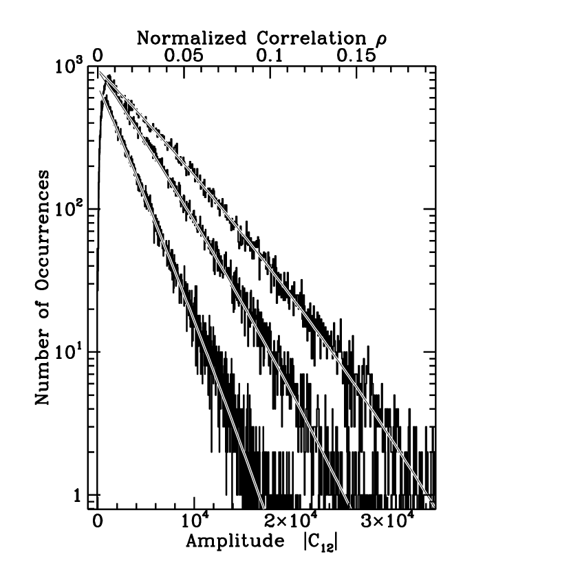
Figure 9: Histogram of distribution of amplitude in 3 gates, with the best-fitting distribution for the distribution of normalized correlation, as given by Eq. 23 and shown in Figure 4. Table 3 gives parameters of the fit. The distributions are concave downward because of correlator normalization, as discussed in § 2.5.

Normalization of the correlation detectably affects the distribution of amplitude for the Vela pulsar. Figure 9 shows the distributions of amplitude in the 3 gates, with a logarithmic vertical axis. A purely exponential distribution would follow a straight line on this plot, but the observed distribution falls below this line at both small and large amplitudes. The figure shows the best-fitting models including effects of normalization of the correlation (Eq. 23) for each gate, which accurately describe the distributions at large amplitude. Table 3 summarizes results of the fits of the distribution expected for a normalized correlation function, given by Eq. 23, to the data in Fig. 9. To improve the sensitivity of the fit to the high end of the distribution, we fit to the logarithm of the histogram. The fitted parameters agree well with expectations. The normalization is greater than the number of data in the histogram, probably because of the reduction in the distribution at small amplitudes by effects of noise and finite source size.

Models including effects of finite size and noise (Eq. 2.3.3) accurately describe the distributions at low amplitudes, where these effects become important, as Figure 7 shows. If we compare the parameters of the 2 distributions at the intermediate amplitudes where both take a nearly exponential form, using the approximations in Eqs. 17 and 24, unsurprisingly we find that they agree very well, as Figure 9 would suggest.

5 Discussion

5.1 Size of the Pulsar’s Emission Region

Our analysis indicates a decreasing size across the pulse. Table 4 summarizes our results, expressed both in terms of the size parameter, and as the FWHM of the best-fitting Gaussian distribution, in km. To calculate the size in km from the results of the fit requires the additional parameters $k$, $M$, and $\theta_{\xi}$, $\theta_{\eta}$. The angular broadening of the pulsar is $\theta_{\xi}\times\theta_{\eta}=(3.3\pm 0.2~{}{\rm mas})\times(2.0\pm 0.1~{}{\rm mas})$, with the major axis at a position angle of $92^{\circ}\pm 10^{\circ}$ (Gwinn et al. (1997)).

We use comparison of our measured decorrelation bandwidth from § 4.2, $\Delta\nu=66\pm 1$ Hz, with the angular broadening and the pulsar distance of $500\pm 100$ pc (Taylor, Manchester, & Lyne (1993)) to obtain the characteristic distance of scattering material (Desai et al. (1992), Gwinn, Bartel, & Cordes (11993)). We find that the fractional distance of the scattering material from the Earth to the pulsar is $D/(D+R)=0.60\pm 0.05$. Here recall that $D$ is the distance from observer to scatterer, and $R$ is the distance from scatterer to pulsar. We thus obtain the magnification $M=1.5\pm 0.3$.

We then use the fitted values for the size parameter $(kM\theta_{\xi}\sigma_{s})$ to find the size in km in each gate, given in Table 4. Note that the uncertainty in the magnification factor $M$ dominates the quoted uncertainties of the size. The uncertainty in the magnification factor stems, in turn, primarily from uncertainty in the distance to the pulsar,

The fitted size is in reasonable agreement with our earlier results for gate 1 (Gwinn et al. (1997)). The major differences in the analysis are the accounting for effects of averaging in time and frequency, for the effects of spectrally-varying signals on noise, and our use of the measured decorrelation bandwidth to determine the magnification factor, in this paper.

5.2 Size and Emission Mechanism

Among the 4 classes of processes for pulsar emission discussed by Melrose (1996), the measured size of about 440 km rules out only models in which the observed emission comes from close to the polar cap. This region has a size of less than a km, much smaller than the observed size. If the emission originates at this location, but is transported to a larger region, such models are still viable.

Perhaps because pulsar radiation is collimated into a beam, many pictures of pulsar emission treat the radiation as emerging in only a single direction from each point of the emitting surface, perhaps along the local magnetic field. However, for the emission region to have the size we measure, the observer must receive radiation from points at the emission surface separated by $\sim 400$ km. The observer measures the separations between these points as the size of the emission region. Figure 10 illustrates this fact. Of course, different emitting regions could contribute at different times, so that the emitting region is a point at any instant, and the finite size is observed only by averaging over many points. Our measured size is averaged over 10 s of observations, or 112 pulses, and over a range of pulse phase.

Aberration can significantly affect the observed size of the emission region. At a fraction of the radius of the light cylinder, the pulsar’s magnetosphere travels at a fraction of lightspeed. This can affect the interpretation of the measured size. In particular, the measured size can include the height of the emission region. Figure 10 shows an example. Aberration is particularly important in models where radiation is emitted at a range of heights.

Models for emission at a small fraction of the radius of the light cylinder, $R_{L}=4250$ km, agree naturally with our observation. For a simple dipole field, the open field lines have a cross-section of about 440 km at an altitude of about 450 km. However, sources that emit at a range of altitudes can have measured sizes that include effects of the spread in altitude, so that emission could arise at altitudes of 0 to 440 km, for example. Models for emission from near or at the light cylinder could also produce the observed size, although in that case some physical process must limit the emission to a region less than 10% of the diameter of the light cylinder in size.

The size, and its decrease across the pulse, are in approximate agreement with the results of Krishnamohan & Downs (1983). They concluded that the emission early in the pulse arose from a larger region than that late in the pulse, and that the spread in altitude of emission was about 400 km. Although their methodology was quite different, their picture of the emission region has remarkably similar dimensions.

The measured size is large for “core” emission, which is believed to arise near the stellar surface (Rankin (1990)), because it statistically reflects the opening angle of the dipole field lines at the polar cap. If Vela’s pulse does show core emission, as some suggest, this leads to an apparent paradox. The third gate, with size consistent with zero, might represent the core emission, with the leading edge of the pulse one side of a cone. Studies of size of the emission region as a function of frequency, and imaging of the source, may resolve this question. Measurements of size for other pulsars would also be extremely valuable. Such observations are now in progress.

Arons & Barnard (1986) pointed out that radiation traveling nearly along pulsars’ magnetic field lines, with polarization in the plane defined by the pulsar’s magnetic field and the radiation’s wavevector (the “O-mode”), interacts with the outflowing electron-positron wind. This radiation can be “ducted” along field lines (Barnard & Arons (1986)). In principle, such ducting can lead to a large apparent emission region even though the original source of radiation, perhaps near the pulsar’s polar cap, is quite compact. Lyutikov (1998b) points out that microphysics can amplify, as well as refract, these waves.

Magnetospheric refraction takes place for only one polarization. The Vela pulsar is heavily linearly polarized, so this picture and the size measurements suggests that the dominant polarization represents the O-mode. However, the less-dominant polarization mode is present, and should show zero size if magnetospheric refraction sets the size. Thus, polarimetric size measurements suggest a simple test of whether magnetospheric refraction is responsible for the observed size. Such measurements should be little more difficult than those described here, and are presently being pursued.

6 Summary

We present measurements of the size of the radio emission region of the Vela pulsar, from the observed distribution of correlation amplitude on a short interferometer baseline. In strong scintillation, this distribution is exponential if the source is pointlike, and is the sum of 3 exponentials if the source is small but extended (Gwinn et al. (1998)). The effects of finite size on this distribution are concentrated at small amplitudes. We find that averaging in frequency and time has effects similar to those of finite size. We calculate the distribution including effects of Gaussian noise in the observing system, when an interferometer observes the source. This effect is likewise greatest at the lowest amplitudes, with a different functional form. We calculate the expected effects of variations in pulsar flux density and in instrumental gain: these effects tend to make the distribution more sharply peaked at zero amplitude and flatter at high amplitudes, and are small unless the variations in gain approach 100%. We calculate the effects of self-noise, which likewise make the distribution function higher at low amplitudes and flatter at high amplitudes, and are important when the number of independent samples, $N_{q}$, is small. We finally consider the effect of normalization of the correlation function, and find that this makes the distribution function fall more rapidly than the exponential extrapolated from small amplitudes, when the correlation approaches 100%.

We compare model distributions of amplitude with that observed for the Vela pulsar on the Parkes-Tidbinbilla baseline at $\lambda=13$ cm. We measure the noise level, and the variation in gain with frequency channel, from observations of a strong continuum source. Models including a finite size for the pulsar in all 3 gates provide good fits. We correct the fitted sizes for the effects of averaging in frequency and time. The fitted size parameters are significant at about 10 times the standard errors, depending on the gate. Table 2 summarizes the results. The size decreases across the pulse. We find that effects of gain and pulsar flux-density variations, self-noise, the Van Vleck correction, and averaging in time and frequency are expected to be undetectably small for our observation. Effects of normalization of the correlation function are detected, but do not significantly affect the size estimates. The linear size of the pulsar’s emission region is about 440 km in the first gate, 340 km in the second, and less than 200 km in the third.

We discuss size measurements for sources that, like pulsars, radiate into a collimated beam. The measured size is the size of the region on the source visible to the observer; that size may not be identical from all lines of sight, so that the measured size may easily change as the source rotates, as we observe. Aberration effects may also affect the measured size, so that the range in altitude of the emission region, as well as its width, may contribute to the size.

Our measured size is much larger than the sizes of postulated polar-cap emission regions, so that such models, without additional physics, are ruled out for this pulsar. However, magnetospheric refraction can duct radiation from a compact emission region to produce a much larger size (Arons & Barnard (1986), Barnard & Arons (1986)). The observed size is on the order of postulated emission regions in the lower open-field-line region, suggesting that this is a likely location for pulsar emission. It is much smaller than the outer open-field-line region or the light cylinder, but emission might arise in only parts of these regions, or might be beamed toward the observer from only certain parts.

Figure 1: Probability distribution $P(S)$ for flux density $S$, for a point source (dotted line), and for sources with small size $\sigma_{s}$ ($kM\theta_{\xi}\sigma_{s}=0.15$: solid line) and with larger size ($kM\theta\sigma_{s}=0.40$: long-dashed line). Vertical lines near the top of the figure indicate the scales $S_{1\xi}$, $S_{1\xi}$, and $S_{0}$ for the smaller source; those near the bottom indicate these scales for the larger source. The mean flux density is the same for all 3 sources; $<S>=1$. In these examples, the elongation of the scattering disk is $\theta_{\xi}/\theta_{\eta}=1.4$.

Figure 2: Upper panel: Distribution of amplitude of correlation, $|{\bf C}_{12}|$ for a scintillating point source, observed by 2 identical antennas, including effects of system noise and self-noise (see Eq. 2.3.1). The mean flux density of the source is $S_{0}=1$. The signal-to-noise ratio (excluding self-noise) is $\Gamma S_{0}N_{q}^{1/2}/T_{s}=10$ or $2$, as indicated for the 2 families of curves. For each family, the number of samples $N_{q}$ is $3000$ (solid line), $30$ (dotted line), and $10$ (dashed line). The system temperature is $T_{s}$ and the antenna temperature is $\Gamma S_{0}$. Effects of self-noise are greatest when the signal is large compared with noise, and $N_{q}$ is small. Lower panel: The same curves, plotted on a logarithmic scale.

Figure 3: Expected distributions of amplitude of correlation for a scintillating point source, including effects of variations in instrumental gain (or, equivalently, intrinsic variations in flux density). The solid curve shows the exponential distribution expected for a point source in strong scintillation, with mean and exponential scale equal to the mean amplitude of the source, 1 in this example. Variations in gain change this distribution by superposing distributions with different exponential scales. The model distributions of gain are flat, extending from 0.8 to 1.2 times the mean (dotted curve) and from 0 to 2 times the mean (dashed curve). Distributions with significant contributions at zero or very low gain differ the most from the case of constant gain.

Figure 4: Probability distribution of normalized correlation $\rho_{0}$, and scaled 2-bit correlation ${\textstyle{{\pi}\over{2}}}\rho_{2}$, for a strongly-scintillating source with exponential distribution of flux density. The average flux density, and scale of the exponential distribution, is $S_{0}$. Antenna temperature is $\Gamma S_{0}$, and system temperature is $T_{S}$, so $\Gamma S_{0}/T_{S}$ is signal-to-noise ratio for a single sample. For each of 3 values of $\Gamma S_{0}/T_{s}$, the probability distribution is shown for the normalized correlation $\rho_{0}$ (solid curve: Eq. 23); the scaled 1-bit correlation ${\textstyle{{\pi}\over{2}}}\rho_{2}$ (dashed curve: Eq. 25, with $\eta=1$); and the limiting exponential form for small correlation (dotted curve: Eq. 24). The curves differ only when the source is strong relative to system noise. All forms assume that $N_{q}$ is large so that self-noise can be ignored.

Figure 5: Gain plotted with frequency in a typical 2-MHz recorded band. Data are for the extragalactic continuum source 0826$-$373, observed from 00:22:50 to 00:35:30 UT on 1992 Nov 1, between 2286.99 and 2288.99 MHz on the Tidbinbilla-Parkes baseline. The data were averaged coherently for 10 s in time and 25 kHz in frequency, and then averaged incoherently in time for the entire 13-minute scan. To reduce effects of gain variations, we use only data from the central portion of the band, between the vertical lines.

Figure 6: Histogram of noise. Data are the same as in Fig. 5. To remove the effects of gain variations on the relatively high amplitude of the source, we subtracted the average amplitude given in Table 1 from the data in each band, and then added the overall average amplitude of 1500. Thus, the histogram reflects noise rather than gain differences among the bands. The solid curve shows the best-fitting Gaussian distribution, with parameters given in Table 1.

Figure 7: Histograms of observed amplitude in 3 gates across the pulsar pulse. For each gate, the right panel shows the histogram of amplitudes with the best-fitting model (solid curve) and the model with zero size (dotted curve). Inset shows the pulse profile with the gate. The left panel shows residuals from the model with zero size, for the data (histogram) and for the best-fitting model (solid curve). The decrease in pulse intensity, as the gates progress across the pulse, appears as a decrease in the scale of the exponentials, from the top panel (Gate 1) to the bottom panel (Gate 3).

Figure 8: Fitted size parameter, plotted as a function of averaging in time and frequency, in Gate 2. The size is normalized to the resolution of the scattering disk acting as a lens, expressed as $(kM\theta_{\xi}\sigma_{s})$. The ordinate is the averaging bandwidth: 25 kHz as produced by the correlator, and boxcar averages to 50 and 75 kHz. Circles show fits for data averaged by 5 sec in time, squares by 10 sec, and triangles by 15 sec. The 4 curves show the predictions of the best-fitting model with parameters of decorrelation bandwidth $\Delta\nu=66$ kHz and scintillation timescale $t_{ISS}=26$ sec. The different curves show predictions for averaging in time by 0, 5, 10, or 15 sec. Section 2.2 describes the model.

Figure 10: Upper: Observed size of a source of beamed radiation. If the source radiates in a single direction from each point, an observer sees only a single point. For example, if the source radiates only along the solid arrows, an observer at top sees only point “c”. If the source emits in a range of directions at each point, the observer measures a finite size. For example, if each point radiates into the angle shown by the dotted lines, an observer at top sees radiation from points “b” through “d” and measures size $L$ for the emission region. Lower: Effects of aberration on measured source size. The emission region rotates with the pulsar, at left, at angular frequency $\Omega$. Points on the surface of the emission region radiate into narrow cones toward the right, in the rotating frame. Aberration redirects radiation so that it travels along the dotted paths from the lower emitting point, and dashed paths from the upper emitting point. An observer above the source measures a size for the emission region comparable to its height.

Table 1: Fits to Noise

		Average
Band	Noise	Amplitude	Normalization
	$\sigma$	$\bar{|C|}$
1	$78.3\pm 1.2$	$1459.9\pm 1.2$	$4414\pm 60$
2	$76.8\pm 1.1$	$1479.8\pm 1.0$	$4387\pm 52$
3	$75.7\pm 1.5$	$1510.4\pm 1.5$	$4405\pm 78$
4	$74.6\pm 0.8$	$1524.8\pm 0.8$	$4386\pm 43$
5	$76.6\pm 1.2$	$1499.8\pm 1.1$	$4384\pm 58$
6	$73.4\pm 1.0$	$1498.5\pm 0.9$	$4392\pm 49$
All	$74.3\pm 1.0$	$1499.6\pm 1.1$	$26260\pm 320$

Table 2: Fits to Distributions of Intensity of the Vela Pulsar

Parameter		Gate 1	Gate 2	Gate 3
Fixed Parameters
Number of Data		$74492$	$69305$	$74076$
Bin Width		$50$	$75$	$25$
Assumed Noise Level		$558.6$	$507.7$	$474.9$
Fitted Parameters
Size Parameter	$(kM\theta_{\xi}{\bar{\sigma}}_{s})^{2}$	$0.173\pm 0.005$	$0.163\pm 0.005$	$0.149\pm 0.005$
Amplitude	$S_{0}$	$4395\pm 56$	$6185\pm 104$	$2826\pm 23$
Normalization		$76804\pm 537$	$72441\pm 742$	$75631\pm 340$
Standard Deviation of Residuals		$12.29$	$20.49$	$17.99$
Size Parameter
After Correction for Averaging	$(kM\theta_{\xi}\sigma_{s})^{2}$	$0.091\pm 0.009$	$0.070\pm 0.012$	$0.020\pm 0.020$

Table 3: Fits for Normalized Correlation

Parameter		Gate 1	Gate 2	Gate 3
Conversion factor	$|C_{12}|/(\rho_{0}/\eta)$	$(5.6\pm 1.4)\times 10^{-6}$	$(5.6\pm 1.4)\times 10^{-6}$	$(5.6\pm 1.4)\times 10^{-6}$
Normalization		$77640\pm 1212$	$73430\pm 746$	$78756\pm 1086$
Scale	$\Gamma S_{0}/T_{s}$	$0.0233\pm 0.0002$	$0.0324\pm 0.0004$	$0.0152\pm 0.0001$

Table 4: Size of the Vela Pulsar

		Gate 1	Gate 2	Gate 3
Size Parameter
Corrected for Averaging	$(kM\theta_{\xi}\sigma_{s})$	$0.091\pm 0.009$	$0.070\pm 0.009$	$0.020\pm 0.020$
Size (FWHM)	$\sqrt{8\ln 2}\sigma_{s}$	$440\pm 90$ km	$340\pm 80$ km	$100\pm 100$ km

References

- Arons (1983) Arons, J. 1983, ApJ, 266, 215
- Arons & Barnard (1986) Arons, J., & Barnard, J.J. 1986, ApJ, 302, 120
- Asseo (1996) Asseo, E. 1996, in IAU Colloq. 160, Pulsars: Problems and Progress, ed. S. Johnston, M.A. Walker, and M. Bailes, San Francisco: Astronomical Society of the Pacific, p. 147
- Backer (1974) Backer, D.C. 1974, ApJ, 190, 667
- Backer (1975) Backer, D.C. 1975, A&A, 43, 395
- Barnard & Arons (1986) Barnard, J.J., & Arons, J. 1986, ApJ, 302, 138
- Bartz (1993) Bartz, M. 1993, Microwaves & RF, 32, 5:192
- Blandford & Scharlemann (1976) Blandford, R.D., & Scharlemann, E.T. 1976, MNRAS, 174, 59
- Britton (1997) Britton, M.C. 1997, PhD Thesis, University of California, Santa Barbara
- Codona et al. (1986) Codona, J.L., Creamer, D.B., Flatté, S.M., Frehlich, R.G., & Henyey, F.S. 1986, Radio Science, 21, 805
- Cordes, Weisberg & Boriakoff (1983) Cordes, J.M., Weisberg, J.M., & Boriakoff, V. 1983, ApJ, 268, 370
- Cordes, Weisberg & Boriakoff (1985) Cordes, J.M., Weisberg, J.M., & Boriakoff, V. 1985, ApJ, 288, 221
- Cordes (1998) Cordes, J.M. 1998, personal communication
- Cornwell et al. (1989) Cornwell, T.J., Anantharamaiah, K.R., & Narayan, R. 1989, JOSA, A 6, 977
- Desai et al. (1992) Desai, K.M., Gwinn, C.R., Reynolds, J.R., King, E.A., Jauncey, D., Flanagan, C., Nicolson, G., Preston, R.A., & Jones, D.L. 1992, ApJ, 393, L75
- Goldreich & Julian (1969) Goldreich, P., & Julian, W.H. 1969, ApJ, 157, 869
- Goodman (1985) Goodman, J.W. 1985, Statistical Optics, New York: Wiley
- Gwinn, Bartel, & Cordes (11993) Gwinn, C.R., Bartel, N., Cordes J.M. 1993, ApJ, 410, 673
- Gwinn et al. (1997) Gwinn, C.R., Ojeda, M.J., Britton, M.C., Reynolds, J.E., Jauncey, D.L., King, E.A., McCulloch, P.M., Lovell, J.E.J., Flanagan, C.S., Smits, D.P., Preston, R.A., & Jones, D.L. 1997, ApJ, 483, L53
- Gwinn et al. (1998) Gwinn, C.R., Britton, M.C., Reynolds, J.E., Jauncey, D.L., King, E.A., McCulloch, P.M., Lovell, J.E.J., & Preston, R.A. 1998, ApJ, 505, 928
- Gwinn et al. (1999) Gwinn, C.R., et al. 1999, in preparation.
- Hankins (1972) Hankins, T.H. 1972, ApJ, 177, L11
- (23) Jenet, F.A., & Anderson, S.B. 1998, PASP, 110, 1467
- Krishnamohan & Downs (1983) Krishnamohan, S., & Downs, G.S. 1983, ApJ, 265, 372
- Lyne & Manchester (1988) Lyne, A.G., & Manchester, R.N. 1988, MNRAS, 234, 477
- Lyne & Graham-Smith (1998) Lyne, A.G., & Graham-Smith, F. 1998, Pulsar astronomy , 2nd ed., Cambridge: Cambridge University Press
- (27) Lyutikov, M. 1998a, MNRAS, 293, 447
- (28) Lyutikov, M. 1998b, MNRAS, 298, 1198
- Manchester (1995) Manchester, R.N. 1995, JApA, 16, 107
- Melrose (1996) Melrose, D.B. 1996, in IAU Colloq. 160, Pulsars: Problems and Progress, ed. S. Johnston, M.A. Walker, and M. Bailes San Francisco: Astronomical Society of the Pacific, p. 139
- Melrose & Stoneham (1977) Melrose, D.B. and Stoneham, R.J., 1977, Proc. Astr. Soc. Australia, 3, 120
- Meyer (1975) Meyer, S.L. 1975, Data Analysis for Scientists and Engineers, New York: Wiley
- Press et al. (1989) Press, W.H., Flannery, B.P., Teukolsky, S.A., & Vetterling, W.T. 1989, Numerical Recipes, Cambridge UK: Cambridge Univ. Press
- Radhakrishnan & Cooke (1969) Radhakrishnan, V., & Cooke, D.J. 1969, ApLett, 3, 225
- Radhakrishnan & Rankin (1990) Radhakrishnan, V., & Rankin, J.M. 1990, ApJ, 352, 258
- Rankin (1983) Rankin, J.M. 1983, ApJ, 274, 333
- Rankin (1986) Rankin, J.M. 1986, ApJ, 301, 901
- Rankin (1990) Rankin, J.M. 1990, ApJ, 352, 247
- Rickett (1975) Rickett, B.J. 1975, ApJ, 197, 185
- Roberts & Ables (1982) Roberts, J.A., & Ables, J.G. 1982, MNRAS, 201, 1119
- Romani & Yadigaroglu (1995) Romani, R.W., & Yadigaroglu, I.A. 1995, ApJ, 438, 314
- Ruderman & Sutherland (1975) Ruderman, M.A. & Sutherland, P.G. 1975, ApJ, 196, 51
- Scheuer (1968) Scheuer, P.A.G. 1968, Nature, 218, 920
- Smirnova et al. (1996) Smirnova, T. V., Shishov, V. I., Malofeev, V. M. 1996, ApJ, 462, 289
- Strickman et al. (1996) Strickman, M.S., Grove, J.E., Johnson, W.N., Kinzer, R.I., Kroeger, R.A., Kurfess, J.D., Grabelsky, D.A., Matz, S.M., Purcell, W.R., Ulmer, M.P., & Jung, G.V. 1996, ApJ, 460, 735
- Sturrock (1971) Sturrock, P.A. 1971, ApJ, 164, 529
- Taylor, Manchester, & Lyne (1993) Taylor, J.H., Manchester, R.N., & Lyne, A.G. 1993, ApJSS, 88 529
- Thompson, Moran, & Swenson (1986) Thompson, A.R., Moran, J.M., & Swenson, G.W. Jr. 1986, Interferometry and Synthesis in Radio Astronomy, (New York: Wiley)
- Weatherall & Eilek (1997) Weatherall, J.C. & Eilek, J.A. 1997, ApJ, 474, 407
- Wolszczan & Cordes (1987) Wolszczan, A. & Cordes, J.M. 1987, ApJ, 320, L35