Formation and Disruption of Cosmological Low Mass Objects

Abstract

We investigate the evolution of cosmological low mass (low virial temperature) objects and the formation of the first luminous objects. First, the ‘cooling diagram’ for low mass objects is shown. We assess the cooling rate taking into account the contribution of H₂, which is not in chemical equilibrium generally, with a simple argument of time scales. The reaction rates and the cooling rate of H₂ are taken from the recent results by Galli & Palla (1998). Using this cooling diagram, we also estimate the formation condition of luminous objects taking into account the supernova (SN) disruption of virialized clouds. We find that the mass of the first luminous object is several $\times 10^{7}M_{\odot}$, because smaller objects may be disrupted by the SNe before they become luminous. Metal pollution of low mass (Ly-$\alpha$) clouds also discussed. The resultant metallicity of the clouds is $Z/Z_{\odot}\sim 10^{-3}$.

1 Introduction

Today, we have a great deal of observational data concerning the early universe. However, we have very little information about the era referred to as the ‘dark ages’. Information regarding the era of recombination (with redshift $z$ of about $10^{3}$) can be obtained by the observation of cosmic microwave background radiation. After the recombination era little information is accessible until $z\sim 5$, after that we can observe luminous objects such as galaxies and QSOs. On the other hand, the reionization of the intergalactic medium and the presence of heavy elements at high-$z$ suggest that there are other population of luminous objects, which precedes normal galaxies. Thus, theoretical approach to reveal the formation mechanism of the such unseen luminous objects is very important.

It is now widely accepted that luminous objects are formed from overdense regions in the early universe. These overdense regions collapse to form luminous objects, in case they fragment into many stellar size clouds and many massive stars are formed. In order to understand the way in which luminous objects are formed, physical processes of the clouds in various stages of evolution should be studied, individually.

The formation process of luminous objects is roughly divided into three steps, formation of cold clouds by H and/or ${\rm H_{2}}$ line cooling, formation of the first generation stars in the cold clouds, and the star formation throughout the host clouds. These steps are disturbed by the feedback from the first stars. The first step has been investigated by many authors (e.g., Haiman, Thoul & Loeb (1996); Ostriker & Gnedin (1996); Tegmark et al. (1997); Gnedin & Ostriker (1997); Abel et al. (1998)) and it has been shown that the low mass clouds (virial temperature is several $\times 10^{3}$ K) become the earliest cooled dense clouds. The second step, however, is not investigated enough, although initial mass function and formation efficiency of the first generation stars in the clouds are very challenging and crucial problems. Many authors attacked this problem (Matsuda, Sato & Takeda (1969); Hutchins (1976); Carlberg (1981); Palla, Salpeter & Stahler (1983); Uehara et al. (1996)) and they obtained various conclusions. However, now, the mass of the first generation stars are estimated through detailed investigation to be fairly large (Nakamura & Umemura (1999); Omukai & Nishi (1998)). For the third step, the feedback from the luminous objects on the other clouds has been studied by several authors (Haiman, Rees & Loeb (1996, 1997); Ferrara (1998); Haiman, Abel & Rees (1999)). Haiman, Abel & Rees (1999) examined the build-up of the UV background in hierarchical models and its effects on star formation inside small halos that collapse prior to reionization. They stressed that early UV background below 13.6 eV suppresses the H₂ abundance and there exists a negative feedback even before reionization. Moreover, the feedback from the formed stars on their own host cloud is more serious. The main feedback consists of two different processes, UV radiation from the stars and energy input by SNe. Through ionization of H (Lin & Murray (1992)) and dissociation of H₂ (Silk (1977); Omukai & Nishi (1999)), UV radiation have negative feedback on the further star formation in the host clouds. Especially, H₂ is dissociated in such a large region that the whole of an ordinary low mass cloud is influenced by one O5 type star (Omukai & Nishi (1999)). The feedback from SNe on the host clouds is probably negative (e.g., Mac Low & Ferrara (1999)). SNe can disrupt the host clouds before they become luminous, because the explosion energy is comparable with the typical binding energy of host clouds. In this Letter, we investigate the evolution of low mass primordial clouds systematically, and assess the mass of the first luminous objects.

2 Cooling diagram

The formation of cold dense clouds, i.e., progenitors of luminous objects, is basically understood by the comparison between free-fall time and the cooling time. The ‘cooling diagram’ originally introduced by Rees & Ostriker (1977) and Silk (1977) shows the region where cooling time is shorter than the free-fall time on $\rho$ - $T$ plane, and vice versa. In this section, we present the cooling diagram on $\rho$ - $T$ plane including H₂ cooling. With this diagram, we can predict whether a cloud virialized at $z=z_{\rm vir}$ with virial temperature $T_{\rm vir}$ cools.

2.1 H₂ fraction with given virial temperature

In order to estimate the cooling rate at $T<10^{4}$K, we need the fraction of H₂. The number fraction of H₂ (hereafter denoted as $y_{\rm H_{2}}$) is not generally in equilibrium for $T<10^{4}$ K in the epoch of galaxy formation. The value of $y_{\rm H_{2}}$ at a time depends not only on $\rho$ and $T$ but also on the initial condition. Consequently, we cannot evaluate the cooling rate on the $\rho$ - $T$ plane without estimating non-equilibrium $y_{\rm H_{2}}$. Tegmark et al. (1997) calculate $y_{\rm H_{2}}$ numerically, however, their primordial $y_{\rm H_{2}}$ is about two orders of magnitude over estimated because the destruction rate of ${\rm H_{2}^{+}}$ by cosmic microwave background radiation at high-$z$ is under estimated (Galli & Palla (1998)). Since their primordial value $\sim 10^{-4}$ is comparable to the necessary value to cool, their cooling criterion is not reliable generally. Here, using recent reaction rates and the cooling rate of H₂ (Galli & Palla (1998)), we adopt a simplified and generalized method to estimate the cooling function of H₂, differently from that of Tegmark et al. (1997). We introduce four important time scales, $t_{\rm dis}$, $t_{\rm form},t_{\rm cool},$ and $t_{\rm rec}$. They represent dissociation and formation time of H₂, cooling time, and recombination time, respectively. Comparing these time scales, we assess the non-equilibrium fraction of H₂ with given virial temperature, and redshift. Below, our estimation is summarized (see Fig. 1a).

1. The case $t_{\rm dis}<{\rm min}(t_{\rm cool},t_{\rm rec})$ (Region of “$t_{\rm dis}$ fastest” in Fig. 1a): H₂ is in chemical equilibrium. In this case, $y_{\rm H_{2}}=y_{\rm H_{2}}^{\rm eq}$, where $y_{\rm H_{2}}^{\rm eq}$ denotes the fraction of H₂ in chemical equilibrium (solution of $t_{\rm form}=t_{\rm dis}$).

2. The case $t_{\rm rec}<{\rm min}(t_{\rm cool},t_{\rm dis})$ (Region of “$t_{\rm rec}$ fastest” in Fig. 1a): H₂ is out of chemical equilibrium, and H₂ molecules are formed until the recombination process significantly reduces the electron fraction. As a result, $y_{\rm H_{2}}$ is determined by the equation, $t_{\rm form}=t_{\rm rec}$. Combined with the relation $t_{\rm form}=y_{\rm H_{2}}/y_{\rm H_{2}}^{\rm eq}t_{\rm dis}$(Susa et al. (1998)), $y_{\rm H_{2}}$ is obtained as, $y_{\rm H_{2}}=y_{\rm H_{2}}^{\rm eq}\left(t_{\rm rec}/t_{\rm dis}\right)$.

3. The case $t_{\rm cool}<{\rm min}(t_{\rm rec},t_{\rm dis})$ (Region of “$t_{\rm cool}$ fastest” in Fig. 1a): When the cooling time is the shortest of the three time scales, $y_{\rm H_{2}}$ is determined by the equation $t_{\rm form}=t_{\rm cool}$. In other words, $y_{\rm H_{2}}$ increases until the system is cooled significantly. In case $y_{\rm H_{2}}$ cooling dominates the other cooling processes, $y_{\rm H_{2}}\simeq y_{\rm H_{2}}^{\rm eq}\sqrt{t_{\rm cool}^{\rm eq}/t_{\rm dis}}$. Otherwise, $y_{\rm H_{2}}$ is the solution of a quadratic equation. Here, $t_{\rm cool}^{\rm eq}$ represents cooling time scale by H₂ rovibrational transitions with $y_{\rm H_{2}}^{\rm eq}$.

The electron fraction of a virialized cloud is assumed as $y_{e}={\rm max}(y_{e}^{\rm rel},y_{e}^{\rm eq})$. Here $y_{e}^{\rm rel}$ is the fraction of cosmologically relic electrons calculated in Galli & Palla (1998). It equals to $3.02\times 10^{-4}$ for their standard model. The chemical equilibrium fraction of electrons is denoted $y_{e}^{\rm eq}$. With this electron fraction, we estimate the fraction of H₂.

In Fig. 1b, $y_{\rm H_{2}}$ is plotted with given virial temperatures for four redshifts. For low redshift ($z\mathrel{\mathchoice{\lower 2.15277pt\vbox{\halign{$\mathsurround 0pt \displaystyle\hfil#\hfil$\cr<\crcr\sim\crcr}}}{\lower 2.15277pt\vbox{\halign{$\mathsurround 0pt \textstyle\hfil#\hfil$\cr<\crcr\sim\crcr}}}{\lower 2.15277pt\vbox{\halign{$\mathsurround 0pt \scriptstyle\hfil#\hfil$\cr<\crcr\sim\crcr}}}{\lower 2.15277pt\vbox{\halign{$\mathsurround 0pt \scriptscriptstyle\hfil#\hfil$\cr<\crcr\sim\crcr}}}}100$) and high temperature ($T\simeq 10^{4}$K), H₂ is in chemical equilibrium with given ionization degree. As the temperature drops, H₂ gets out of equilibrium because the cooling time becomes shorter than the other time scales. Below $2000$ K, recombination time scale is the shortest, and $y_{\rm H_{2}}$ becomes relic value.

For high redshift, the destruction of H^- ($z\mathrel{\mathchoice{\lower 2.15277pt\vbox{\halign{$\mathsurround 0pt \displaystyle\hfil#\hfil$\cr>\crcr\sim\crcr}}}{\lower 2.15277pt\vbox{\halign{$\mathsurround 0pt \textstyle\hfil#\hfil$\cr>\crcr\sim\crcr}}}{\lower 2.15277pt\vbox{\halign{$\mathsurround 0pt \scriptstyle\hfil#\hfil$\cr>\crcr\sim\crcr}}}{\lower 2.15277pt\vbox{\halign{$\mathsurround 0pt \scriptscriptstyle\hfil#\hfil$\cr>\crcr\sim\crcr}}}}100$) and H${}^{+}_{2}$ ($z\mathrel{\mathchoice{\lower 2.15277pt\vbox{\halign{$\mathsurround 0pt \displaystyle\hfil#\hfil$\cr>\crcr\sim\crcr}}}{\lower 2.15277pt\vbox{\halign{$\mathsurround 0pt \textstyle\hfil#\hfil$\cr>\crcr\sim\crcr}}}{\lower 2.15277pt\vbox{\halign{$\mathsurround 0pt \scriptstyle\hfil#\hfil$\cr>\crcr\sim\crcr}}}{\lower 2.15277pt\vbox{\halign{$\mathsurround 0pt \scriptscriptstyle\hfil#\hfil$\cr>\crcr\sim\crcr}}}}200$) by cosmic microwave background radiation reduces $y_{\rm H_{2}}$ significantly.

2.2 Comparison between free-fall time and cooling time

We are able to assess the cooling rate with the given H₂ fraction evaluated in the previous subsection. We compare the time scale of collapse ($t_{\rm ff}$) with the cooling time ($t_{\rm cool}$) which include the contribution from the H₂ cooling. They are,

$$t_{\rm ff}=\left(\frac{3\pi}{32G\rho_{\rm vir}}\right)^{1/2},~{}~{}~{}t_{\rm cool}=\frac{1.5\mu^{-1}kT_{\rm vir}}{n_{\rm vir}\Lambda\left(y_{\rm H_{2}},T_{\rm vir},n_{\rm vir}\right)}.$$ (1)

Here, $\rho_{\rm vir}\equiv 18\pi^{2}\Omega\rho_{\rm cr}$ and $n_{\rm vir}\equiv\Omega_{b}\rho_{\rm vir}/m_{p}$, where $\rho_{\rm cr}\equiv 1.9\times 10^{-29}h^{2}(1+z_{\rm vir})^{3}{\rm~{}g~{}cm}^{-3}$. We adopt $\Omega=1$, $\Omega_{b}=0.06$ and $h=0.5$ in this paper.

Equating $t_{\rm ff}$ and $t_{\rm cool}$ in eq. (1), we obtain the boundary between the cooled region during the collapse and the other region, which is drawn on the $(1+z_{\rm vir})$ - $T_{\rm vir}$ plane in Fig. 2a. The objects virialized into the region denoted as $t_{\rm ff}<t_{\rm cool}$ will be cooled by H₂ during the gravitational collapse. In this case, collapsing cloud will be a mini-pancake, because the thermal pressure becomes negligible. We remark that the cooling region expands into $T_{\rm vir}\mathrel{\mathchoice{\lower 2.15277pt\vbox{\halign{$\mathsurround 0pt \displaystyle\hfil#\hfil$\cr<\crcr\sim\crcr}}}{\lower 2.15277pt\vbox{\halign{$\mathsurround 0pt \textstyle\hfil#\hfil$\cr<\crcr\sim\crcr}}}{\lower 2.15277pt\vbox{\halign{$\mathsurround 0pt \scriptstyle\hfil#\hfil$\cr<\crcr\sim\crcr}}}{\lower 2.15277pt\vbox{\halign{$\mathsurround 0pt \scriptscriptstyle\hfil#\hfil$\cr<\crcr\sim\crcr}}}}10^{4}$K, which is different from classical cooling diagram such as the one in Rees & Ostriker (1977).

We also compare the cooling time scale with the Hubble expansion time ($H^{-1}$). The line $t_{\rm cool}=H^{-1}$ is also drawn on Fig. 2a. The cooling region during the Hubble expansion time is slightly larger than the previous one, because Hubble expansion time is longer than the free-fall time. In this case, the collapse proceeds in semi-statically. As a result, the central region of the cloud will proceed to the run away collapse phase (Tsuribe & Inutsuka (1999)).

3 SNe and disruption of the bound objects

As the collapse proceeds, small amount of the total gas is cooled to $100$K by H₂. In those clouds, massive stars ($10-100M_{\odot}$) will be formed (Nakamura & Umemura (1999); Omukai & Nishi (1998)), eventually. After massive first generation stars form, evolution of the host clouds become slower because of strong regulation by UV radiation (Omukai & Nishi (1998)). Thus, next generation stars are hardly formed before the first generation stars die. Subsequent SNe might disrupt the gas binding before significant amount of total gas transferred into stars. Here, we derive the cloud disruption condition by SNe, with the assumption that the cloud is spherical and the density is constant, for the simplicity.

We estimate the kinetic energy transferred from the SNe to gas. The velocity of expanding shock front from the center of a supernova remnant (SNR) is

$$v_{\rm s}(t)=\left(\frac{7.64\times 10^{-3}\left(\gamma^{2}-1\right)KE}{\rho_{1}}\right)^{1/5}t^{-3/5},$$ (2)

where $K=1.53$, $E$ is the total thermal energy given by the SN, $\rho_{1}$ is the density of the cloud before the explosion, and $t$ denotes the elapsed time since the explosion (Spitzer (1978)). Integrating eq. (2), we obtain the location of the shock front:

$$R_{\rm s}(t)=\left(\frac{0.746\left(\gamma^{2}-1\right)KE}{\rho_{1}}\right)^{1/5}t^{2/5}.$$ (3)

The mass of the hot bubble is also obtained as $m_{\rm SNR}=\frac{4}{3}\pi R_{\rm s}^{3}(t)\rho_{1}$. The hot bubble keeps pushing the surrounding gas until the thermal energy is pumped off by the radiative cooling. Thus, the total momentum transferred from the SNR to the gas cloud is $p_{\rm tot}=m_{\rm SNR}(t_{\rm cool})v_{\rm s}(t_{\rm cool})$. Equating this momentum with the momentum of the whole cloud, we have the expanding velocity of the cloud:

$$v_{\rm tot}=\frac{m_{\rm SNR}\left(t_{\rm cool}\right)}{m_{\rm tot}}v_{s}\left(t_{\rm cool}\right).$$ (4)

If this velocity $v_{\rm tot}$ is smaller than the escape velocity ($v_{\rm esc}$) of the cloud, it will be still bounded. Otherwise, it disrupts. Now, we replace $m_{\rm tot}$ in equation (4) with $m_{\rm J}(T_{\rm vir},z_{\rm vir})$, which is the virialized mass of the cloud collapsed at $z_{\rm vir}$ with $T_{\rm vir}$. The escape velocity from the cloud is directly related to the virial temperature. Consequently, we can draw the disruption boundary ($v_{\rm esc}=v_{\rm tot}$) on the $(1+z_{\rm vir})$ - $T_{\rm vir}$ plane.

On the cooling diagram (Fig. 2a), the boundaries ($v_{\rm esc}=v_{\rm tot}$) are superimposed for two cases. These lines are obtained with the assumption that the input thermal energy from the SNe is $10^{51}$ erg and $10^{52}$ erg, respectively. The input energy almost reflects the number of the SNe. The values $10^{51}$ erg and $10^{52}$ erg represent the case of single SN and $10$ SNe, respectively. The former should corresponds to the clouds in $t_{\rm ff}<t_{\rm cool}<H^{-1}$, because they will have a runaway collapsing central core. The core evolves much faster than the envelope and will be a massive star, probably, followed by a single SN. The latter case represents the clouds in $t_{\rm ff}>t_{\rm cool}$. They will have a shocked pancake, and the cooled region will fragment into stars. That’s why they should have multiple SNe.

However, we should note that the disruption criteria by SNe strongly depend on the geometry of objects (Mac Low & Ferrara (1999); Ciardi et al. (1999) and references there in). In the case that cooling is efficient ($t_{\rm ff}>t_{\rm cool}$), a cloud evolves dynamically and becomes complicated shape, which is probably flattened. The geometric effect makes the momentum transfer from the SNR to the surrounding gas less efficient than our evaluation. On the other hand, if cooling is not efficient ($t_{\rm ff}<t_{\rm cool}$), a cloud becomes fairly spherical and has a centrally condensed density profile. In this case, the effect of SNe may become stronger than the above estimate (e.g., Morgan & Lake (1989)). Moreover, if the duration of the multiple SNe is longer than or comparable with the evolution time scale of a SNR, disruption criteria is not evaluated only with the total energy of multiple SNe (e.g., Ciardi & Ferrara (1997)). Thus, our estimate shows the qualitative tendency, so that detailed calculation for a individual cloud is necessary to derive the SNe effects accurately.

4 Evolution of low mass objects and mass of the first luminous objects

According to the argument in the previous section, the clouds in the region $t_{\rm ff}>t_{\rm cool}$ will experience multiple SNe. Assuming that the total energy of multiple SNe as $10^{52}$ erg, the survived region is the dark shaded upper region of Fig. 2b (denoted as “LO”). As shown in Fig. 2b survived clouds are fairly massive ($T_{\rm vir}\mathrel{\mathchoice{\lower 2.15277pt\vbox{\halign{$\mathsurround 0pt \displaystyle\hfil#\hfil$\cr>\crcr\sim\crcr}}}{\lower 2.15277pt\vbox{\halign{$\mathsurround 0pt \textstyle\hfil#\hfil$\cr>\crcr\sim\crcr}}}{\lower 2.15277pt\vbox{\halign{$\mathsurround 0pt \scriptstyle\hfil#\hfil$\cr>\crcr\sim\crcr}}}{\lower 2.15277pt\vbox{\halign{$\mathsurround 0pt \scriptscriptstyle\hfil#\hfil$\cr>\crcr\sim\crcr}}}}10^{4}$ K) and they evolve into luminous objects through following processes (Nishi et al. (1998)): (1) By pancake collapse of an overdense region or collision between subclouds in a potential well, a quasi-plane shock forms (e.g., Susa, Uehara & Nishi (1996)). (2) If the shock-heated temperature is higher than $\sim 10^{4}$ K, the post-shock gas is ionized and cooled efficiently by H line cooling. After it is cooled bellow $10^{4}$ K, ${\rm H_{2}}$ is formed fairly efficiently and it is cooled to several hundred K by ${\rm H_{2}}$ line cooling (e.g., Shapiro & Kang (1987); Susa et al. (1998)). (3) The shock-compressed layer fragments into cylindrical clouds when $t_{\rm dyn}\sim t_{\rm frag}$ (Yamada & Nishi (1998); Uehara & Nishi (1999)). (4) The cylindrical cloud collapses dynamically and fragments into cloud cores when $t_{\rm dyn}\sim t_{\rm frag}$ (Uehara et al. (1996); Nakamura & Umemura (1999)). (5) Primordial stars form in cloud cores (Omukai & Nishi (1998)). (6) Since the gravitational potential of the cloud is deep enough, subsequent SNe cannot disrupt the cloud. Star formation regulation by UV radiation is also weak because of highly flattened configuration of the host cloud. (7) Next generation stars can form efficiently and the cloud evolves into a luminous object.

On the other hand, the clouds in the region $t_{\rm ff}<t_{\rm cool}<H^{-1}$ will experience a single SN. As a result, the survived region is bounded by the line denoted as $10^{51}$ erg (denoted as “Ly-$\alpha$” of Fig. 2b) and they evolve into luminous objects if they are isolated. However, the evolution time scale of these clouds is rather long because of large disturbance by the SN and they are reionized at low-$z$. After reionization, they may be observed as Ly-$\alpha$ clouds. Since the baryonic mass of these clouds are several $\times 10^{5}M_{\odot}$ and the ejected metal mass by a SN is several $M_{\odot}$, their metallicity is estimated to be $\sim 10^{-3}Z_{\odot}$. The observation of QSO absorption line systems imply the similar metallicity for Ly-$\alpha$ clouds (Cowie et al. (1995); Songaila & Cowie (1996); Songaila (1997); Cowie & Songaila (1998)). They are typically the 1$\sigma$ objects and collapse at $z\sim 10$. Our estimate basically agrees with the more detailed calculation in Ciardi & Ferrara (1997).

In the unshaded lower right region ($T_{\rm CMB}>T_{\rm vir}$) and the lightly shaded region “NC” of Fig. 2b, clouds are diffuse and do not become luminous, because radiative cooling is not efficient. In the shaded region “IG”, SNe destroy the binding of host objects, followed by the diffusion of heavy elements into the surrounding medium.

Therefore, the first luminous objects are probably formed in the region “LO” and their mass is estimated to be several $\times 10^{7}M_{\odot}$, if we consider the $2\sim 3\sigma$ objects. Formation epoch of the first luminous objects is $z\sim 30$ (considering the 3$\sigma$ objects) or $z\sim 20$ (considering the 2$\sigma$ objects). This estimated mass is larger than the one obtained by Tegmark et al. (1997), because small clouds may be blown up by their own SNe.

Figure 1: (a) The $y_{e}$ - $T$ plane is divided into three region. In the region with higher temperature, $t_{\rm dis}$ is the fastest and $y_{\rm H_{2}}=y_{\rm H_{2}}^{\rm eq}$. In the region with lower temperature, $t_{\rm rec}$ is the fastest and $y_{\rm H_{2}}=y_{\rm H_{2}}^{\rm eq}{t_{\rm rec}\over t_{\rm dis}}$. Between these two regions, where $t_{\rm cool}$ is the fastest, $y_{\rm H_{2}}\simeq y_{\rm H_{2}}^{\rm eq}\sqrt{\frac{t_{\rm cool}^{\rm eq}}{t_{\rm dis}}}$. (b) Virial temperature v.s. H₂ fraction is plotted for given epoch of collapse ($z$).

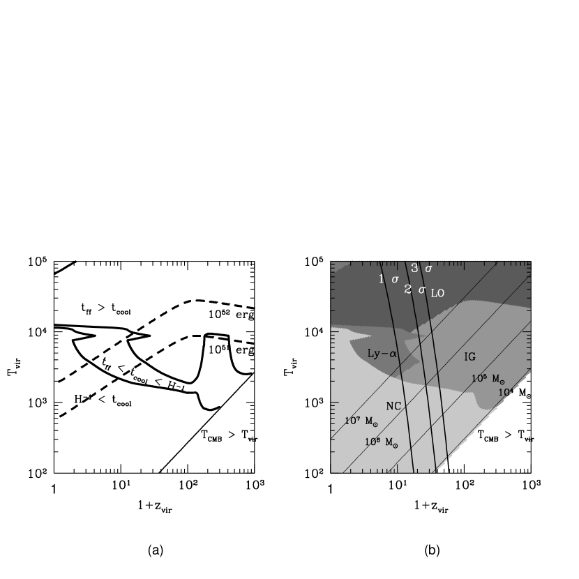
Figure 2: (a) Cooling diagram is plotted on the $(1+z_{\rm vir})$ - $T_{\rm vir}$ plane. The thick solid lines divide the plane into three regions. In the region denoted as $t_{\rm ff}>t_{\rm cool}$, cooling proceeds faster than the collapse. The narrow region denoted as $t_{\rm ff}<t_{\rm cool}<H^{-1}$, the cloud cools faster than the Hubble expansion, but cannot catch up with the free-fall. The clouds virialized into the lower region ($H^{-1}<t_{\rm cool}$), cannot cool and will not be the luminous objects. The lower right region ($T_{\rm CMB}>T_{\rm vir}$) is the forbidden region of cooling, due to the Compton heating. Two dashed lines denote the boundary below which virialized clouds are destroyed by SN explosions. The lines correspond to the cases that the total energy of SNe is $10^{51}$ erg and $10^{52}$ erg. (b) $(1+z_{\rm vir})$ - $T_{\rm vir}$ plane is divided into five regions. In the unshaded lower right region ($T_{\rm CMB}>T_{\rm vir}$) and the lightly shaded region denoted as “NC”, clouds are diffuse and do not become luminous, because radiative cooling is not efficient. In the shaded region denoted as “IG”, clouds will be disrupted by the SNe. Clouds in the region “Ly-$\alpha$” will not be destroyed by the SN. The dark shaded upper region (denoted as “LO”), represents the clouds which could be luminous objects. The thick solid three lines marked as $1\sigma$, $2\sigma$, and $3\sigma$ represent the location that the density perturbations in standard CDM cosmology should virialize. The mass of the clouds are constant along the thin solid four lines which cross the panel from lower left to upper right. The lines correspond to the total masses are $10^{4}M_{\odot}$, $10^{5}M_{\odot}$, $10^{6}M_{\odot}$, and $10^{7}M_{\odot}$.

References

- Abel et al. (1998) Abel T., Steebbins, A., Anninos, P. & Norman M. L. 1998, ApJ, 508, 530
- Carlberg (1981) Carlberg R. G. 1981, MNRAS, 197, 1021
- Ciardi & Ferrara (1997) Ciardi B. & Ferrara 1997, ApJ, 483, L5
- Ciardi et al. (1999) Ciardi B., Ferrara, A. Governato F. and Jenkins, A. 1999, submitted to MNRAS, astro-ph/9907189
- Cowie et al. (1995) Cowie, L. L., Songaila, A., Kim, T.,& Hu, E. M. 1997, AJ, 109, 1522
- Cowie & Songaila (1998) Cowie,L.L., & Songaila, A. 1998, Nature, 394, 44
- Ferrara (1998) Ferrara A. 1998, ApJ, 499, L17
- Galli & Palla (1998) Galli D. & Palla F. 1998, A&A, 335, 403
- Gnedin & Ostriker (1997) Gnedin N. Y. & Ostriker J. P. 1997, ApJ, 486, 581
- Haiman, Abel & Rees (1999) Haiman Z., Abel, T. & Rees M. 1999, submitted to ApJ, astro-ph/9903336
- Haiman, Thoul & Loeb (1996) Haiman Z., Thoul A. A. & Loeb A. 1996, ApJ, 464, 523
- Haiman, Rees & Loeb (1996) Haiman Z., Rees M. & Loeb A. 1996, ApJ, 467, 522
- Haiman, Rees & Loeb (1997) Haiman Z., Rees M. & Loeb A. 1997, ApJ, 476, 458
- Hutchins (1976) Hutchins, J. B. 1976, ApJ, 205, 103
- Lin & Murray (1992) Lin D. N. C. & Murray S. D. 1992, ApJ, 394, 523
- Mac Low & Ferrara (1999) Mac Low, M.-M. & Ferrara, A. 1999, ApJ, 513, 142
- Matsuda, Sato & Takeda (1969) Matsuda T., Sato H. & Takeda H. 1969, Prog. Theor. Phys. 42, 219
- Morgan & Lake (1989) Morgan, S. & Lake G. 1989, ApJ, 339, 171
- Nakamura & Umemura (1999) Nakamura F. & Umemura M. 1999, ApJ, 515, 239
- Nishi et al. (1998) Nishi R., Susa H., Uehara H., Yamada M. & Omukai K. 1998, Prog. Theor. Phys., 100, 881
- Omukai & Nishi (1998) Omukai K. & Nishi R. 1998, ApJ, 508, 141
- Omukai & Nishi (1999) Omukai K. & Nishi R. 1999, ApJ, 518, 64
- Ostriker & Gnedin (1996) Ostriker J. P. & Gnedin N. Y. 1996, ApJ, 472, L63
- Palla, Salpeter & Stahler (1983) Palla F., Salpeter E. E. & Stahler S. W. 1983 ApJ, 271, 632
- Rees & Ostriker (1977) Rees M. J. & Ostriker J. P. 1977, MNRAS, 179, 541
- Shapiro & Kang (1987) Shapiro P. R. & Kang H. 1987, ApJ, 318, 32
- Silk (1977) Silk J. 1977, ApJ, 211, 638
- Songaila & Cowie (1996) Songaila, A. & Cowie, L.L. 1996, AJ, 112, 335
- Songaila (1997) Songaila, A. 1997, ApJ, 490, L1
- Spitzer (1978) Spitzer L. Jr. 1978, Physical Processes in the Interstellar Medium (John Willey, New York)
- Susa, Uehara & Nishi (1996) Susa H., Uehara H. & Nishi R. 1996, Prog. Theor. Phys., 96, 1073
- Susa et al. (1998) Susa H., Uehara H., Nishi R. & Yamada M. 1998, Prog. Theor. Phys., 100, 63
- Tegmark et al. (1997) Tegmark M., Silk J., Rees M. J. Blanchard A., Abel T. & Palla F. 1997, ApJ, 474, 1
- Tsuribe & Inutsuka (1999) Tsuribe T. & Inutsuka S. 1999, ApJ, in press
- Uehara & Nishi (1999) Uehara H. & Nishi R. 1999, ApJ, accepted
- Uehara et al. (1996) Uehara H., Susa H., Nishi R., Yamada M. & Nakamura T. 1996, ApJ, 473, L95
- Yamada & Nishi (1998) Yamada M. & Nishi R. 1998, ApJ, 505, 148