Interactions in Scalar Field Cosmology

Abstract

We investigate spatially flat isotropic cosmological models which contain a scalar field with an exponential potential and a perfect fluid with a linear equation of state. We include an interaction term, through which the energy of the scalar field is transferred to the matter fields, consistent with a term that arises from scalar–tensor theory under a conformal transformation and field redefinition. The governing ordinary differential equations reduce to a dynamical system when appropriate normalized variables are defined. We analyse the dynamical system and find that the interaction term can significantly affect the qualitative behaviour of the models. The late-time behaviour of these models may be of cosmological interest. In particular, for a specific range of values for the model parameters there are late-time attracting solutions, corresponding to a novel attracting equilibrium point, which are inflationary and in which the scalar field’s energy-density remains a fixed fraction of the matter field’s energy density. These scalar field models may be of interest as late-time cosmologies, particularly in view of the recent observations of the current accelerated cosmic expansion. For appropriate values of the interaction coupling parameter, this equilibrium point is an attracting focus, and hence as inflating solutions approach this late-time attractor the scalar field oscillates. Hence these models may also be of importance in the study of inflation in the early universe.

Pacs 98.80.Cq

1 Introduction

A variety of theories of fundamental physics predict the existence of scalar fields [1, 2, 3], motivating the study of the dynamical properties of scalar fields in cosmology. Indeed, scalar field cosmological models are of great importance in the study of the early universe, particularly in the investigation of inflation [4, 2]. Recently there has also been great interest in the late-time evolution of scalar field models. ‘Quintessential’ scalar field models (or slowly decaying cosmological constant models) [5, 6] give rise to a residual scalar field which contributes to the present energy-density of the universe that may alleviate the dark matter problem and can predict an effective cosmological constant which is consistent with observations of the present accelerated cosmic expansion [7, 8].

Models with a self-interaction potential with an exponential dependence on the scalar field of the form

$$V=\Lambda e^{k\phi},$$ (1)

where $\Lambda$ and $k$ are positive constants, have been the subject of much interest and arise naturally from theories of gravity such as scalar-tensor theories or string theories [3]. Recently, it has been argued that a scalar field with an exponential potential is a strong candidate for dark matter in spiral galaxies [9] and is consistent with observations of current accelerated expansion of the universe [10].

A number of authors have studied scalar field cosmological models with an exponential potential within general relativity. Homogeneous and isotropic Friedmann-Robertson-Walker (FRW) models were studied by Halliwell [11] using phase-plane methods. Homogeneous but anisotropic models of Bianchi types I and III (and Kantowski-Sachs models) were studied by Burd and Barrow [12], Bianchi type I models were studied by Lidsey [13] and Aguirregabiria et al. [14], and Bianchi models of types III and VI were studied by Feinstein and Ibáñez [15]. A qualitative analysis of Bianchi models with $k^{2}<2$ (including standard matter satisfying standard energy conditions) was completed by Kitada and Maeda [16]. The governing differential equations in spatially homogeneous Bianchi cosmologies containing a scalar field with an exponential potential reduce to a dynamical system when appropriate expansion- normalized variables are defined. This dynamical system was studied in detail in [17] (where matter terms were not considered).

One particular solution that is of great interest is the flat, isotropic power-law inflationary solution which occurs for $k^{2}<2$. This power-law inflationary solution is known to be an attractor for all initially expanding Bianchi models (except a subclass of the Bianchi type IX models which will recollapse) [16, 17]. Therefore, all of these models inflate forever; there is no exit from inflation and no conditions for conventional reheating.

Recently cosmological models which contain both a scalar field with an exponential potential and a barotropic perfect fluid with an equation of state

$$p=(\gamma-1)\mu,$$ (2)

where $\gamma$ is in the physically relevant range $2/3<\gamma\leq 2$, have come under heavy analysis. One class of exact solutions found for these models has the property that the energy density due to the scalar field is proportional to the energy density of the perfect fluid, and hence these models have been labelled matter scaling cosmologies [18, 19, 20]. These matter scaling solutions are spatially flat isotropic models and are known to be late-time attractors (i.e., stable) in the subclass of flat isotropic models [18, 19, 20] and are clearly of physical interest. In addition to the matter scaling solutions, curvature scaling solutions [21] and anisotropic scaling solutions [22] are also possible. A comprehensive analysis of spatially homogeneous models with a perfect fluid and a scalar field with an exponential potential has recently been undertaken [23].

Within the standard model of inflation (with, for example, a quadratic or quartic self-interaction potential), in the early universe the microphysics of the scalar field leads to an accelerated expansion essentially driven by the potential energy (or vacuum energy) that arises when the scalar field is displaced from its potential energy minimum. Provided that the potential is sufficiently flat, the universe undergoes many e-folds of expansion and the matter content is driven to zero [24, 25, 26, 27, 28]. As the scalar field nears its minimum, the vacuum energy is converted to coherent oscillations of the scalar field (which corresponds to non-relativistic scalar particles). Eventually, since the scalar field is coupled to other (fermionic and bosonic) matter fields, these particles decay into lighter particles and their thermalization results in the ‘reheating’ of the universe (thereby accounting for the current entropy in the universe today).

Although the exponential models are interesting models for a variety of reasons, they have some shortcomings as inflationary models. While Bianchi models generically asymptote towards the power-law inflationary model in which the matter terms are driven to zero for $k^{2}<2$, there is no graceful exit from this inflationary phase. Furthermore, the scalar field cannot oscillate and so reheating cannot occur by the conventional scenario. Clearly, these models need to be augmented in an attempt to alleviate these problems. For example, exponential potentials are only believed to be an approximation, and so the theory could include more complicated potentials (although it is not clear what these other potentials should be).

The goal of this paper is to examine how interaction terms, through which the energy of the scalar field is transferred to the matter fields, can affect the qualitative behaviour of models containing matter and a scalar field with an exponential potential. Such an interaction term, denoted by $\delta$, arises in the conservation equations, via

$$\dot{\phi}\left(\ddot{\phi}+3H\dot{\phi}+kV\right)=-\delta$$ (3a)

$$\dot{\mu}+3\gamma H\mu=\delta.$$ (3b)

The form of such a term has been discussed in the literature within the context of inflation and reheating. An alternative to the conventional reheating model, in which the scalar field’s energy is transferred to the matter due to scalar field oscillations, is the warm inflationary model [29, 30, 20] in which an interaction term is significant throughout the inflationary regime (not just after slow-roll) and so the energy of the scalar field is continually transferred to the matter content throughout inflation and the matter content is not driven to zero.

Several examples of interaction terms appear in the literature for models with a variety of self-interaction potentials. In particular, potentials which have a global minimum have attracted much attention. For example, Albrecht et al. [31] considered $\delta=a\dot{\phi}^{d}\phi^{5-2d}$ (where $a$ is a constant), derived from dimensional arguments, in the reheating context after inflation (with potentials derived from Georgi–Glashow SU(5) models). In a similar context, Berera [32] considered interaction terms of the form $\delta=a\dot{\phi}^{2}$. Quadratic potentials and interaction terms of the form $\delta=a\dot{\phi}^{2}$ and $\delta=a\phi^{2}\dot{\phi}^{2}$ were considered by de Oliveira and Ramos [33] and a graceful exit from inflation was demonstrated numerically. Similarly, Yokoyama et al. [34] showed that an interaction term, which is negligible during the slow-roll inflationary phase, dominates at the end of inflation when the scalar field is oscillating about its minimum; during this reheating phase it is assumed that the energy transferred from the scalar field is solely converted into particles.

Within the context of exponential potentials, Yokoyama and Maeda [35] and Wands et al. [19] considered interactions of the form $\delta=a\sqrt{V}$. The main goal in both these papers was to show that power-law inflation can occur for $k^{2}>2$, thereby showing that inflation can exist for steeper potentials. The main motivation for this work is the fact that exponential potentials which arise naturally from other theories, such as supergravity or superstring models, typically have $k^{2}>2$. Wetterich [36] considered interaction terms containing a matter dependence, namely $\delta=a\dot{\phi}\mu$, in which perturbation analysis showed that the matter scaling solutions were stable solutions when such interaction terms are included. In [36], it was shown that the age of the universe is older when $\delta$ is included and that the scalar field can still significantly contribute to the energy density of models at late times. In [3], certain string theories in which the energy sources are separately conserved in the Jordan frame naturally lead to interaction terms in the Einstein frame, although this is not specific to string cosmologies; any scalar-tensor theory with matter terms and a power-law potential will yield the same results [36].

The scalar field in scalar–tensor theory can be related to the scalar field in the general relativistic scalar field theory via a conformal transformation. If the matter terms are separately conserved in the scalar–tensor theory (Jordan frame) then they lead to the following conservation equation in the Einstein Frame

$$\dot{\phi}\left(\ddot{\phi}+3H\dot{\phi}+kV\right)=\frac{\left(4-3\gamma\right)}{2\sqrt{\omega+\frac{3}{2}}}\dot{\phi}\mu$$ (4)

(and a similar equation for $\dot{\mu}$), where $\omega$ is the coupling parameter in the scalar–tensor theory. This therefore leads to an interaction term of the form $\delta=-a\dot{\phi}\mu$, where

$$a=\frac{\left(4-3\gamma\right)}{2\sqrt{\omega+\frac{3}{2}}}.$$ (5)

Similarly, in string theory ($\omega=-1$), a similar interaction term arises in the Einstein frame which depends on the energy density of the matter (axion) field and $a$ is of order unity. Finally, a term of the form $\delta=a\mu H$ might be motivated by analogy with dissipation. For example, a fluid with bulk viscosity may give rise to a term of this form in the conservation equation [37].

If $\delta$ does not depend on the matter energy-density, then unphysical situations may arise. For conventional interaction terms without $\mu$, we have found numerically that $\mu$ is driven to zero in a finite time and subsequently the matter energy-density becomes negative (see [3] for details). Thus, we shall include a factor $\mu$ in the interaction term in order to ensure that $\mu\geq 0$. In [36] it was shown that if $\delta<0$ at the equilibrium points then static solutions (i.e. $\dot{\phi}=0$) are not possible. Furthermore, we require that the sign of $\delta$ be positive at equilibrium points representing inflationary phases, otherwise the matter fields will be “feeding” the scalar field and will redshift to zero even faster than in the absence of the interaction terms.

This paper examines interaction terms of the general form $\delta=\bar{\delta}\mu H$ (where $\bar{\delta}=\bar{\delta}(\dot{\phi},V,H)$) in the context of flat FRW models with emphasis in determining the asymptotic properties of these models. In particular, it will be determined whether these models can asymptote towards inflationary models in which the matter terms are not driven to zero. This would partially alleviate the need for reheating; since the matter content tracks that of scalar field (in this context) it is never driven to zero (unless both are driven to zero in which case the solution is not inflationary). However, a more comprehensive reheating model would still be necessary. The structure of the paper is as follows. In section 2, the governing equations are defined and the case $\delta=0$ studied in [38] is reviewed. In section 3, the case $\delta=a\dot{\phi}\mu$ is studied, motivated by the conformal relationships between the Jordan and Einstein frame in string theory, and extends the work of [36]. In section 4 we shall discuss the results of the analysis and in section 5 we shall examine an interaction term of the form $\delta=a\mu H$. The paper ends with conclusions in section 6.

2 Governing Equations

The governing field equations are given by the equations (LABEL:conserve_interact) and

$$\dot{H}=-\frac{1}{2}(\gamma\mu+\dot{\phi}^{2}),$$ (6)

subject to the Friedmann constraint

$$H^{2}=\frac{1}{3}(\mu+\frac{1}{2}\dot{\phi}^{2}+V),$$ (7)

(an overdot denotes ordinary differentiation with respect to time $t$). Note that the total energy density of the scalar field is given by $\mu_{\phi}=\frac{1}{2}\dot{\phi}^{2}+V$. The deceleration parameter for this system is given by

$$q=\frac{1}{3}H^{-2}\left[\dot{\phi}^{2}-V+\frac{1}{2}\left(3\gamma-2\right)\mu\right],$$ (8)

and is independent of the interaction term.

Defining

$$x\equiv\frac{\dot{\phi}}{\sqrt{6}H}\quad,\quad y\equiv\frac{\sqrt{V}}{\sqrt{3}H},$$ (9)

and the new logarithmic time variable $\tau$ by

$$\frac{d\tau}{dt}\equiv H,$$ (10)

the governing differential equations can be written as the plane-autonomous system:

$$x^{\prime} = -3x-\sqrt{\frac{3}{2}}ky^{2}+\frac{3}{2}x[2x^{2}+\gamma(1-x^{2}-y^{2})]-\frac{\bar{\delta}}{6x}(1-x^{2}-y^{2}),$$ (11a)

$$y^{\prime} = \frac{3}{2}y\left[\sqrt{\frac{2}{3}}kx+2x^{2}+\gamma(1-x^{2}-y^{2})\right],$$ (11b)

where a prime denotes differentiation with respect to $\tau$ [3]. Note that $y=0$ is an invariant set, corresponding to $V=0$. The equations are invariant under $y\rightarrow-y$ and $t\rightarrow-t$ and so the region $y<0$ is a time-reversed mirror of the region $y>0$; therefore, only $y>0$ will be considered. Similarly, only $k>0$ will be considered since the equations for the interaction terms to be considered are invariant under $k\rightarrow-k$ and $x\rightarrow-x$.

Equation (7) can be written as

$$\Omega+\Omega_{\phi}=1,$$

where

$$\Omega\equiv\frac{\mu_{\gamma}}{3H^{2}},\quad\Omega_{\phi}\equiv\frac{\mu_{\phi}}{3H^{2}}=x^{2}+y^{2},$$ (12)

which implies that $0\leq x^{2}+y^{2}\leq 1$ for $\Omega\geq 0$ so that the phase-space is bounded. The deceleration parameter is now written

$$q=-1+3x^{2}+\frac{3}{2}\gamma\left(1-x^{2}-y^{2}\right).$$ (13)

2.1 Comments on arbitrary $\bar{\delta}$

The fact that $q$ is independent of the interaction term implies that the region of phase space which represents inflationary models is the same for all of the models considered. Namely, $q=0$ occurs along the ellipse $\gamma y^{2}=(2-\gamma)x^{2}+\frac{1}{3}(3\gamma-2)$. For any value of $\gamma$, the lines intersect the boundary of the phase space at $x^{2}=\frac{1}{3}$.

It is possible to make some qualitative comments about the system (11a) for arbitrary $\bar{\delta}$. First, the location of equilibrium points on the boundary $x^{2}+y^{2}=1$ ($\Omega=0$) are independent of the choice of such interaction terms; the three equilibrium points (and their associated eigenvalues) which exist on the boundary for any $\bar{\delta}$ are:

$${\cal K}^{+}: (x,y)=(+1,0)$$

$$\left(\lambda_{1},\lambda_{2}\right)=\left(3(2-\gamma)+\frac{1}{3}\left.\bar{\delta}\right|_{{\cal K}^{+}},\sqrt{\frac{3}{2}}\left[\sqrt{6}+k\right]\right),$$

$${\cal K}^{-}: (x,y)=(-1,0)$$

$$\left(\lambda_{1},\lambda_{2}\right)=\left(3(2-\gamma)+\frac{1}{3}\left.\bar{\delta}\right|_{{\cal K}^{-}},\sqrt{\frac{3}{2}}\left[\sqrt{6}-k\right]\right),$$

$$P_{\cal S}: (x,y)=\left(-\frac{k}{\sqrt{6}},\sqrt{1-k^{2}/6}\right)$$

$$\left(\lambda_{1},\lambda_{2}\right)=\left(-\frac{1}{2}\left[6-k^{2}\right],-\left[3\gamma-k^{2}-\frac{1}{3}\left.\bar{\delta}\right|_{P_{\cal S}}\right]\right).$$

The points ${\cal K}^{\pm}$ represent the isotropic subcases of Jacobs’ Bianchi type I solutions [39] (subcases of the Kasner models), generalized to include a massless scalar field. These solutions are non-inflationary ($q=2$). The point $P_{\cal S}$, which exists only for $k^{2}<6$, represents the FRW power-law model [11, 17] and is inflationary for $k^{2}<2$ ($q=\frac{1}{2}\left[k^{2}-2\right]$). Although these three points exists for any $\bar{\delta}$, the interaction term does affect the stability of these solutions, as is evident from the eigenvalues in (2.1). In particular, for $k^{2}<3\gamma$ the point $P_{\cal S}$ can become a saddle point if

$$\left.\bar{\delta}\right|_{P_{\cal S}}>3\left(3\gamma-k^{2}\right).$$

Hence, if the interaction term is significant, solutions will spend an indefinite period of time near this power-law inflationary model, but will then evolve away and typically be attracted to another equilibrium point in some other region of the phase space.

Matter scaling solutions (i.e. those solutions in which $\gamma_{\phi}=\gamma$), denoted by ${\cal F}_{\cal S}$ in [23], exist only in special circumstances when such interaction terms are present, and occur at the point

$$x_{{\cal F}_{\cal S}}=-\sqrt{\frac{3}{2}}\frac{\gamma}{k},\qquad y_{{\cal F}_{\cal S}}=\sqrt{\frac{3\gamma(2-\gamma)}{2k^{2}}}.$$ (15)

Substituting these solutions into equations (11a) yields

$$x^{\prime} = \frac{(3\gamma-k^{2})}{3\sqrt{6}k\gamma}\left.\bar{\delta}\right|_{{\cal F}_{\cal S}},$$ (16a)

$$y^{\prime} = 0.$$ (16b)

Hence, the matter scaling solutions will be represented by an equilibrium point only if $\left.\bar{\delta}\right|_{{\cal F}_{\cal S}}=0$ (or in the special case $3\gamma=k^{2}$, which is typically a bifurcation value). For the simple forms for $\delta$ given in the literature and those used in this paper, this condition will not be satisfied and so the matter scaling solutions cannot be asymptotic attracting solutions.

However, an analogous situation does arise. In particular, any equilibrium point within the boundary of the phase space will satisfy

$$y_{0}^{2}=\frac{(2-\gamma_{\phi})}{\gamma_{\phi}}x_{0}^{2},$$ (17)

in which the scalar field is equivalent to a perfect fluid of the form $p_{\phi}=(\gamma_{\phi}-1)\mu_{\phi}$, but where $\gamma_{\phi}\neq\gamma$. Consequently, any attracting equilibrium point within the phase space will represent models in which neither the matter field nor the scalar field is negligible and the scalar field mimics a barotropic fluid different from the matter field and therefore could still constitute a possible dark matter candidate.

Finally, it can be shown that any equilibrium point within (but not on) the boundary will occur for $x_{0}<0$. For $y\neq 0$ and $\Omega\neq 0$ equation (11b), which does not depend on $\delta$, yields

$$\gamma y^{2}=\gamma+\sqrt{\frac{2}{3}}kx+(2-\gamma)x^{2},$$ (18)

a relationship any such equilibrium point must satisfy. Now, $\gamma(y^{2}+x^{2})<\gamma$ since $y^{2}+x^{2}<1$ inside the boundary, and hence (18) yields

$$x\left(x+\frac{k}{\sqrt{6}}\right)<0,$$ (19)

which cannot be satisfied for $x>0$ (since $k>0$).

2.2 Review of the case $\delta=0$

Copeland et al. [38] performed a phase-plane analysis of the system (11a) for $\delta=0$, and found five equilibrium points. One of the equilibrium points (denoted here by $P$) represents a flat, non-inflating FRW model [38], for which $\Omega=1$. For $2/3<\gamma<2$ this point is a saddle in the phase space. The flat FRW matter scaling solution ($F_{\cal S}$) was found to exist for $k^{2}>3\gamma$ and was shown to be a sink. The equilibrium point ${\cal K}^{+}$ was shown to be a source for all $k$ and ${\cal K}^{-}$ a source for $k^{2}<6$. The FRW power-law model ($P_{\cal S}$) was shown to be a sink for $k^{2}<3\gamma$, and was shown to represent an inflationary model for $k^{2}<2$. The results found in [38] are summarized in table 1.

	$0\leq k^{2}\leq 2$	$2<k^{2}<6$		$k^{2}>6$
		$k^{2}<3\gamma$	$k^{2}>3\gamma$
$P$	saddle	saddle		saddle
	(NI)	(NI)		(NI)
${\cal K}^{+}$	source	source		source
	(NI)	(NI)		(NI)
${\cal K}^{-}$	source	source		saddle
	(NI)	(NI)		(NI)
$P_{\cal S}$	sink	sink	saddle	DNE
	(I) (for $k^{2}<2$)	(NI)	(NI)
${\cal F}_{\cal S}$	DNE	DNE	sink	sink
			(NI)	(NI)

Table 1: The equilibrium points for $\delta=0$ and their stability for various values of $k$. The label “(NI)” denotes non-inflationary models whereas “(I)” represents inflationary models, and “DNE” is used when an equilibrium point does not exist.

3 Interaction term of the form $\delta=-a\dot{\phi}\mu$

In this section, an interaction term of the form $\delta=-a\dot{\phi}\mu$ (and hence $\bar{\delta}=-a\dot{\phi}/H$) shall be considered. Again, it will be assumed that $k>0$. The explicit sign choice for $\delta$, with the assumption that $a>0$, is to guarantee that all equilibrium points within the phase space will represent models in which energy is being transferred from the scalar field to the perfect fluid, since it was shown that all equilibrium points within the phase space occur for $x<0$ ($\dot{\phi}<0$). Indeed, this is even true for the equilibrium point $P_{\cal S}$ on the boundary $\Omega=0$, since it is located at $x<0$. With this particular choice for $\delta$, equations (11a) become

$$x^{\prime} = -3x(1-x^{2})-\sqrt{\frac{3}{2}}ky^{2}+\left(\frac{3}{2}\gamma x+\sqrt{\frac{3}{2}}a\right)\left(1-x^{2}-y^{2}\right),$$ (20a)

$$y^{\prime} = \frac{3}{2}y\left[\sqrt{\frac{2}{3}}kx+2x^{2}+\gamma(1-x^{2}-y^{2})\right].$$ (20b)

There are five equilibrium points for this system:

1. ${\cal K}^{+}:\qquad(x,y)=(+1,0),\qquad\Omega=0,\qquad q=2.$
   The eigenvalues for this equilibrium point are

   $$\left(\lambda_{1},\lambda_{2}\right)=\left(3(2-\gamma)-\sqrt{6}a,\sqrt{\frac{3}{2}}\left[\sqrt{6}+k\right]\right)$$ (21)

   This equilibrium point is a source for $a<\sqrt{\frac{3}{2}}(2-\gamma)$ and a saddle otherwise.

2. ${\cal K}^{-}:\qquad(x,y)=(-1,0),\qquad\Omega=0,\qquad q=2.$
   The eigenvalues for this equilibrium point are

   $$\left(\lambda_{1},\lambda_{2}\right)=\left(3(2-\gamma)+\sqrt{6}a,\sqrt{\frac{3}{2}}\left[\sqrt{6}-k\right]\right),$$ (22)

   and so ${\cal K}^{-}$ is a source for $k^{2}<6$ and a saddle otherwise.

3. $\displaystyle P_{\cal S}:\qquad(x,y)=\left(-\frac{k}{\sqrt{6}},\sqrt{1-\frac{k^{2}}{6}}\right),\qquad\Omega=0,\qquad q=\frac{1}{2}(k^{2}-2).$
   The eigenvalues for this equilibrium point are

   $$\left(\lambda_{1},\lambda_{2}\right)=\left(-\frac{1}{2}\left[6-k^{2}\right],-\left[3\gamma-k^{2}-ka\right]\right).$$ (23)

   This point exists only for $k^{2}<6$ (when $k^{2}=6$, $P_{\cal S}$ merges with the equilibrium point ${\cal K}^{-}$). Here, $P_{\cal S}$ is a sink for $a<(3\gamma-k^{2})/k$ and a saddle otherwise.

4. $\displaystyle N:\qquad(x,y)=\left(-\sqrt{\frac{3}{2}}\frac{\gamma}{\Delta},\sqrt{\frac{3\gamma(2-\gamma)+2a\Delta}{2\Delta^{2}}}\right),\qquad\Omega=\frac{k\Delta-3\gamma}{\Delta^{2}},$   $\displaystyle q=\frac{3\gamma k-2\Delta}{\Delta},$             
   where $\Delta\equiv k+a>0$. Note that this solution is physical (i.e., $\Omega\geq 0)$ either for $k^{2}>3\gamma$ or for $k^{2}<3\gamma$ and

   $$a\geq(3\gamma-k^{2})/k.$$ (24)

   These solutions were discussed in [36] for $a<k$ and are related to similar power-law solutions discussed in [19]. This model inflates if

   $$a\geq(\frac{3}{2}\gamma-1)k.$$ (25)

   (since only $a<k$ was considered in [36] the solutions therein were not inflationary). For $k^{2}<2$, if condition (24) is satisfied then (25) is automatically satisfied and so these models inflate for $k^{2}<2$. For $2<k^{2}<3\gamma$, if condition (25) is satisfied then (24) is automatically satisfied and therefore models can inflate for $k^{2}>2$ if $a\geq(\frac{3}{2}\gamma-1)k$. For $k^{2}>3\gamma$ there is no constraint on $a$ for the point to exist and therefore whether this models inflates is solely determined by (25). The eigenvalues for this equilibrium point are

   $$\lambda_{\pm} = \frac{-3\left[(2-\gamma)k+2a\right]}{4\Delta}\pm\frac{\sqrt{9\left[(2-\gamma)k+2a\right]^{2}-24\left[3\gamma(2-\gamma)+2a\Delta\right]\left[k\Delta-3\gamma\right]}}{4\Delta},$$ (26)

   and so $N$ is always a sink when it exists. Note that the scalar field acts as a perfect fluid with an equation of state parameter given by

   $$\gamma_{\phi}=\frac{\gamma}{1+\frac{a\Delta}{3\gamma}}<\gamma.$$ (27)

5. $\displaystyle N_{2}:\qquad(x,y)=\left(\sqrt{\frac{2}{3}}\frac{a}{(2-\gamma)},0\right),\qquad\Omega=1-\frac{2a^{2}}{3(2-\gamma^{2})},$  $\displaystyle q=\frac{1}{2}(3\gamma-2)+\frac{a^{2}}{(2-\gamma)}>0.$               
   This equilibrium exists for $a<\sqrt{\frac{3}{2}}(2-\gamma)$ and is a saddle, as determined from its eigenvalues:

   $$\left(\lambda_{1},\lambda_{2}\right)=\left(-\frac{3}{2}[2-\gamma]\left[1-\frac{2a^{2}}{3(2-\gamma)^{2}}\right],\frac{3}{2}\gamma+\frac{a(k+a)}{(2-\gamma)}\right).$$ (28)

Table 2 lists the equilibrium points and their stability for the ranges of $k$ and $a$. As is evident, the presence of the interaction term can substantially change the dynamics of these models. We note that all equilibrium points correspond to self–similar models [40].

	$0<k^{2}<2$		$2<k^{2}<3\gamma$			$3\gamma<k^{2}<6$		$k^{2}>6$
	$a<C_{1}$	$a>C_{1}$	$a<C_{1}$	$C_{1}<a<C_{2}$	$a>C_{2}$	$a<C_{2}$	$a>C_{2}$	$a<C_{2}$	$a>C_{2}$
${\cal K}^{+}$	R for $2a^{2}<3(2-\gamma)^{2}$
(NI)	s for $2a^{2}>3(2-\gamma)^{2}$
${\cal K}^{-}$	R							s
(NI)
$P_{\cal S}$	A	s	A	s				DNE
	(I)	(I)	(NI)	(NI)
$N$	DNE	A	DNE	A	A	A	A	A	A
		(I)		(NI)	(I)	(NI)	(I)	(NI)	(I)
$N_{2}$	s for $2a^{2}<3(2-\gamma)^{2}$
(NI)	DNE for $2a^{2}>3(2-\gamma)^{2}$

Table 2: The equilibrium points for the model with $\delta=-a\dot{\phi}\mu$ and their stability for various values of $k$ and $a$. Note that $C_{1}\equiv(3\gamma-k^{2})/k$ and $C_{2}\equiv(3\gamma-2)k/2$. The symbol “R” denotes when the equilibrium point is a source (repellor), “s” for when it is a saddle, “A” for when it is a sink (attractor), and “DNE” when it does not exist within the particular parameter space. The label “(NI)” denotes non-inflationary models whereas “(I)” represents inflationary models.

4 Discussion

4.1 Inflation

We first note that we can obtain inflationary solutions when $k^{2}>2$, unlike the case in which there is no interaction term. Moreover, we see from Table 2 that these inflationary solutions, corresponding to the equilibrium point $N$ and which occur for $a>\frac{1}{2}(3\gamma-2)k$, are sinks (attractors). This result complements the results of [19, 35] who looked for inflationary solutions for steeper potentials. When $k^{2}<2$ and $0<a<(3\gamma-k^{2})/2$ the power-law inflationary solution corresponding to the equilibrium point $P_{\cal S}$ is again a global attracting solution.

Of particular interest is the case when $k^{2}<2$ and $a>(3\gamma-k^{2})/k>0$, when $P_{\cal S}$ is no longer a sink. Therefore, trajectories approach this equilibrium point (and the models inflate for a definite but arbitrarily large period of time) and eventually asymptote towards the new inflating model corresponding to $N$. For $a\approx(3\gamma-k^{2})/k$, the eigenvalues for $N$ (26) are real and negative and so the attracting solution is represented by an attracting node. However, for $a\gtrsim(3\gamma-k^{2})/2$ this equilibrium point is a spiral node; i.e., trajectories exhibit a decaying oscillatory behaviour as they asymptote towards $N$. (For example, for large $a$ equation (26) becomes $\lambda_{\pm}\approx-\frac{3}{2}\pm\sqrt{-3ak}$, leading to complex eigenvalues.)

An Example

To illustrate this oscillatory nature, an explicit example is chosen with $k=1$ and $\gamma=4/3$ (radiation). The equilibrium points and their respective eigenvalues are:

$${\cal K}^{\pm}: \left(\lambda_{1},\lambda_{2}\right)=\left(\pm\sqrt{6}a+2,\sqrt{\frac{3}{2}}\right),$$ (29a)

$$P_{\cal S}: \left(\lambda_{1},\lambda_{2}\right)=\left(a-3,-\frac{5}{2}\right),$$ (29b)

$$N: (x,y)=\lambda_{\pm}=\frac{-(3a+1)}{2(a+1)}\pm\frac{\sqrt{49+26a+33a^{2}-12a^{3}}}{2(a+1)},$$ (29c)

where $a>3$ in order for $N$ to exist and be a sink and for $P_{\cal S}$ to be a saddle. Note that for $a>3$, $N_{2}$ does not exist, ${\cal K}^{+}$ is a saddle and ${\cal K}^{-}$ is a source. Numerical analysis shows that $N$ is a spiral source for $a\gtrsim 3.65$. Figure 1 depicts this phase space for a typical value of $a$ in this range (for illustrative purposes the value $a=8$ is taken), and the attracting region therein is magnified in figure 2. These figures are typical for other values of $\gamma$ (this comment is important since we note that in the context of conformally transformed scalar-tensor theories, strictly speaking $\delta=0$ for $\gamma=4/3$).

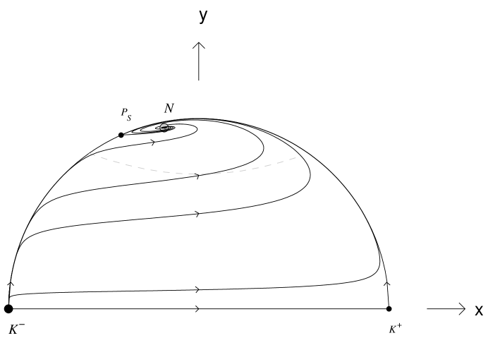
Figure 1: Phase diagram of the system (11a) when $\delta=-a\dot{\phi}\mu$ for the choice of parameters $k=1$, $\gamma=4/3$ and $a=8$. In this figure, the black dot represents the source (i.e., the point ${\cal K}^{-}$), the large grey dot represents the sink (i.e., the point $N$) and small black dots represent saddle points. The region above the grey dashed line represents the inflationary portion of the phase space. Arrows on the trajectory indicate the direction of time.

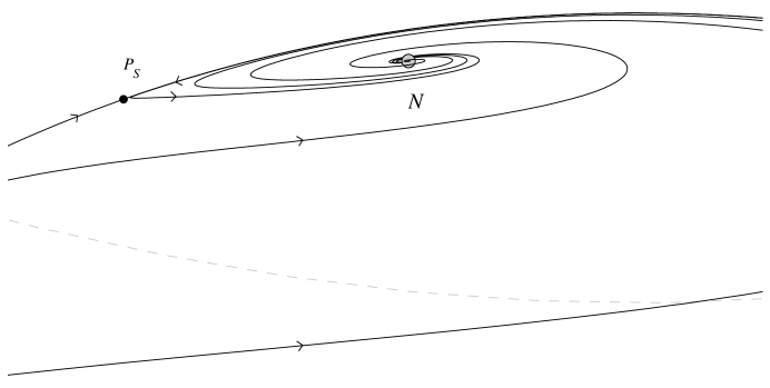
Figure 2: A magnification of the attracting region of the phase space depicted in figure 1. See also caption to figure 1.

4.2 Late-time behaviour

The late-time behaviour of these models, both inflationary and non-inflationary, may also be of cosmological interest. For $2<k^{2}<3\gamma$ & $a<(3\gamma-k^{2})/k$ the late-time attracting equilibrium point is $P_{\cal S}$ which represents a power-law non-inflationary model. Due to recent observations of accelerated expansion [7, 8], models that are presently inflating are also of interest. For $k^{2}<2$ & $a<(3\gamma-k^{2})/k$ the late-time attracting equilibrium point is $P_{\cal S}$ which represents a power-law inflationary model. However, in both of these cases the matter contribution is negligible and so these models are not of physical interest. For $k^{2}<2$ & $a>(3\gamma-k^{2})/k$ the late-time attracting equilibrium point is $N$, which represents a power-law inflationary model in which both the matter and the scalar field are non-negligible and their energy densities are proportional to one another. These models are potentially of great significance, and they have been discussed recently within the scalar-tensor theory context (see below). Finally, for $k^{2}>2$ & $a>(3\gamma-k^{2})/k$ the only late-time attracting equilibrium point is $N$; when $a<(3\gamma-2)k/2$ these models represent non-inflating models whereas the corresponding models inflate for $a>(3\gamma-2)k/2$.

In the absence of an interaction term, matter scaling solutions are represented by equilibrium points of the corresponding dynamical system. We have shown that for simple interaction terms found in the literature, these matter scaling solutions cannot be represented by equilibrium points. However, new equilibrium points arise which represent solutions in which the energy densities of the matter and scalar field remain a fixed proportion to one another and obey $\gamma_{\phi}<\gamma$; these solutions are analogues of the matter scaling solutions in which $\gamma_{\phi}=\gamma$ [36].

In [41] a large class of non-minimally coupled scalar field models with a perfect fluid matter component were investigated. These models contain scalar-tensor theory models and, in particular, Brans-Dicke theory models with a power-law potential. On performing a conformal rescaling of the metric, the governing equations of these models reduce to the equations for a scalar field in general relativity with an exponential potential and an extra coupling to the ordinary matter, and are equivalent mathematically to the equations studies here (as was noted in [3]). Amendola [41] performed a phase space analysis of these models and obtained similar results to those obtained here. (Since Amendola assumed $0<\gamma<2$ he obtained a wider range of possible behaviours; however, these additional results are of lesser interest in the context of our work. In particular, values of $\gamma>4/3$ lead to negative values for the coupling constant a.)

The main aim in [41] was to express the solutions back in the original ‘Jordan’ frame and study the cosmological consequences of the underlying scalar-tensor theory models. In particular, ‘decaying cosmological constant’ solutions were considered which are inflationary and such that the scalar field component is asymptotically non-negligible. Models consistent with the observations of accelerated expansion [7, 8] and in which a physically acceptable fraction of the energy-density is in the scalar field, were found to be severely constrained by the upper limits on the variability of the gravitational constant [42] and by nucleosynthesis observations. In further work Amendola [43] considered a quintessential scalar field coupled to matter with an additional radiation matter component, and studied the effect of density perturbations on the cosmic microwave background in these so-called ‘coupled quintessence’ models.

4.3 Early-time behaviour

From table 2 we can see that the only early-time attractors are ${\cal K}^{\pm}$ for certain values of $k$ and $a$, which correspond to massless scalar field models (which are analogues of Jacob’s vacuum solutions [39]). However, in table 2 we see that for $k^{2}>6$ and $a>\sqrt{\frac{3}{2}}(2-\gamma)$ there are no equilibrium points which represent sources and the trajectories consequently asymptote into the past towards a heteroclinic cycle. In this cycle, orbits quickly shadow the invariant set $x^{2}+y^{2}=1$ ($\Omega=0$), spend a period of time near the saddle ${\cal K}^{-}$, quickly shadow the line $y=0$ ($V=0$, $\Omega\neq 0$), and then spend an period of time near ${\cal K}^{+}$ after which the cycle is repeated. During each cycle the orbits pass through the inflationary portion of phase space. We stress here that this motion is not periodic; on each successive cycle orbits will spend a longer time near the saddles ${\cal K}^{\pm}$. This past-asymptotic qualitative behaviour, which is depicted in figure 3, is similar to that found in [44] within the context of string cosmology; this is not surprising due to the conformal relationship between these string models and the models under investigation here [3].

4.4 The case $\gamma=2$

When $\gamma=2$, corresponding to a stiff perfect fluid, the models is equivalent to a model containing a scalar field with an exponential potential and a second interacting massless scalar field. We also note that $\gamma=2$ is a bifurcation value. The equilibrium points and their eigenvalues in this case are

1. $\displaystyle{\cal K}^{+}:\qquad\left(\lambda_{1},\lambda_{2}\right)=\left(-\sqrt{6}a,\sqrt{\frac{3}{2}}\left[\sqrt{6}+k\right]\right).$
   Since $a>0$ this equilibrium point is a saddle.

2. $\displaystyle{\cal K}^{-}:\qquad\left(\lambda_{1},\lambda_{2}\right)=\left(\sqrt{6}a,\sqrt{\frac{3}{2}}\left[\sqrt{6}-k\right]\right).$
   ${\cal K}^{-}$ is a source for $k^{2}<6$ and a saddle otherwise.

3. $\displaystyle P_{\cal S}:\qquad\left(\lambda_{1},\lambda_{2}\right)=\left(-\frac{1}{2}\left[6-k^{2}\right],-\left[6-k^{2}-ka\right]\right).$
   $P_{\cal S}$ is a source for $a<(6-k^{2})/k$ and a saddle otherwise.

4. $\displaystyle N:\qquad(x,y)=\left(-\sqrt{\frac{6}{\Delta}},\sqrt{\frac{a}{\Delta}}\right),\qquad\Omega=\frac{k\Delta-6}{\Delta^{2}},$   $\displaystyle q=\frac{2\left[2k-a\right]}{\Delta},$             
   where $\Delta\equiv k+a>0$. Note that this solution is physical (i.e., $\Omega\geq 0)$ either for $k^{2}>6$ or for $k^{2}<6$ and $a\geq(6-k^{2})/k$. These models inflate for $k^{2}<2$ as well as for $k^{2}>2$ and $a\geq 2k$. The eigenvalues for this equilibrium point are

   $$\lambda_{\pm} = \frac{-3a}{2\Delta}\pm\frac{\sqrt{9a^{2}-12a\Delta\left[k\Delta-6\right]}}{2\Delta},$$ (30)

   and so $N$ is always a sink when it exists and is a spiral sink for $a>[8k]^{-1}\left[27-8k^{2}+\sqrt{729-48k^{2}}\right]$ or $a<[8k]^{-1}\left[27-8k^{2}-\sqrt{729-48k^{2}}\right]$ (and is a spiral sink for all $k^{2}>6$). Note that the scalar field acts as a perfect fluid with an equation of state parameter given by

   $$\gamma_{\phi}=\frac{2}{1+\frac{1}{6}a\Delta}<\gamma.$$ (31)

Note that the equilibrium point $N_{2}$ does not exist for $\gamma=2$. Table 3 summarizes the stability analysis for $\gamma=2$. The qualitative behaviour is similar to that of the case $\gamma\neq 2$, except that there is no region corresponding to $3\gamma<k^{2}<6$ when $\gamma=2$. Note again that there exists a heteroclinic cycle at early times for $k>\sqrt{6}$ (see Fig. 3); unlike the general case $\gamma\neq 2$, this heteroclinic cycle exists for all $a>0$.

	$0<k^{2}<2$		$2<k^{2}<6$			$k^{2}>6$
	$a<C_{1}$	$a>C_{1}$	$a<C_{1}$	$C_{1}<a<2k$	$a>2k$	$a<2k$	$a>2k$
${\cal K}^{+}$	s
(NI)
${\cal K}^{-}$	R					s
(NI)
$P_{\cal S}$	A	s	A	s		DNE
	(I)	(I)	(NI)	(NI)
$N$	DNE	A	DNE	A	A	A	A
		(I)		(NI)	(I)	(NI)	(I)

Table 3: The equilibrium points for the model with $\delta=-a\dot{\phi}\mu$ and their stability for various values of $k$ and $a$ with $\gamma=2$. Note that $C_{1}\equiv(6-k^{2})/k$. See caption for table 2 for notation.

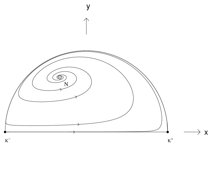
Figure 3: Phase diagram of the system (11a) when $\delta=-a\dot{\phi}\mu$ for the choice of parameters $\gamma=2$ and $k>\sqrt{6}$. Note that the past attractor is a heteroclinic cycle. See also caption to figure2.

5 Interaction term of the form $\delta=a\mu H$

This section provides a second example to demonstrate that other types of interaction terms can also lead to similar behaviour; i.e., that there will be a range of parameters for which the inflationary models which drive the matter fields to zero are not late-time attractors and for which the trajectories exhibit an oscillatory behaviour as they asymptote toward the late-time attracting solution. Specifically, the interaction term $\delta=a\mu H$ is chosen, where $a>0$.

With this choice, equations (11a) become

$$x^{\prime} = -3x(1-x^{2})-\sqrt{\frac{3}{2}}ky^{2}+\left(\frac{3}{2}\gamma x-\frac{a}{2x}\right)\left(1-x^{2}-y^{2}\right),$$ (32a)

$$y^{\prime} = \frac{3}{2}y\left[\sqrt{\frac{2}{3}}kx+2x^{2}+\gamma(1-x^{2}-y^{2})\right].$$ (32b)

For physical reasons we are not interested in early-time behaviour, and hence the line $x=0$ will not be considered. Consequently, a full phase-plane analysis is not possible using these variables. However, it is still possible to determine the equilibrium points with $x\neq 0$ for the system and determine their local stability.

There are four equilibrium points for this system for $x\neq 0$:

1. ${\cal K}^{+}$: Eigenvalues for this equilibrium point are

   $$\left(\lambda_{1},\lambda_{2}\right)=\left(3[2-\gamma]+a,\sqrt{\frac{3}{2}}\sqrt{6}+3\right)$$ (33)

   This equilibrium point is a source.

2. ${\cal K}^{-}$: Eigenvalues for this equilibrium point are

   $$\left(\lambda_{1},\lambda_{2}\right)=\left(3[2-\gamma]+a,-\sqrt{\frac{3}{2}}+3\right).$$ (34)

   ${\cal K}^{-}$ is a source for $k^{2}<6$ and a saddle otherwise.

3. $\displaystyle P_{\cal S}$: Eigenvalues for this equilibrium point are

   $$\left(\lambda_{1},\lambda_{2}\right)=\left(-\frac{1}{2}\left[6-k^{2}\right],-\left[\Xi-k^{2}\gamma-k^{2}\right]\right),$$ (35)

   where $\Xi\equiv 3\gamma-a$. This point exists only for $k^{2}<6$, and is a source for $k^{2}<3\gamma$ and $a<3\gamma-k^{2}$ (saddle otherwise).

4. $\displaystyle N_{1}:\qquad(x,y)=\left(-\frac{\Xi}{\sqrt{6}k},\sqrt{\frac{a}{3\gamma}+\frac{(2-\gamma)}{\gamma}\frac{\Xi^{2}}{6k^{2}}}\right),\qquad\Omega=\frac{\Xi(k^{2}-\Xi)}{3\gamma k^{2}},$  $\displaystyle q=-1+\frac{1}{2}\Xi,$             
   Note that this solution is only physical ($\Omega\geq 0)$ for $[3\gamma-k^{2}]<a<3\gamma$ and $k^{2}<3\gamma$, and represents an inflationary model for $a>(3\gamma-2)$ (consequently, this model will always inflate for $k^{2}<2$ and can inflate for $2<k^{2}<3\gamma$). The eigenvalues for this equilibrium point are

   $$\lambda_{\pm} = -\frac{[2a(2\Xi-k^{2})+(2-\gamma)\Xi^{2}]}{4\gamma\Xi}$$

   $$\pm\frac{\sqrt{\left[2a(2\Xi-k^{2})+(2-\gamma)\Xi^{2}\right]^{2}k^{2}-8\gamma\Xi^{2}(k^{2}-\Xi)\left[2ak^{2}+(2-\gamma)\Xi\right]}}{4\gamma\Delta k},$$

   and so $N_{1}$ is a sink for $a<3\gamma-\frac{1}{2}k^{2}$. Note that the scalar field acts as a perfect fluid with an equation of state parameter given by

   $$\gamma_{\phi}=\frac{\gamma}{1+\frac{ak^{2}}{\Xi^{2}}}<\gamma.$$ (37)

Table 4 lists the equilibrium points and their stability for the ranges of $k$ and $a$. Again, for the range $k^{2}<2$ and $(3\gamma-\frac{1}{2}k^{2})<a<(3\gamma-\frac{1}{2}k^{2})$, the power-law model $P_{\cal S}$ is no longer a sink and $N_{1}$ is a source. Therefore, solutions approach the equilibrium point which is represented by $P_{\cal S}$ (thereby inflating) for an indefinite period of time, but eventually evolve away. It can be shown numerically that within this range for $k$ and $a$, the equilibrium point $N_{1}$ is a spiral node (for instance, for $k=1$ and $\gamma=4/3$, $N_{1}$ is a sink for $3<a<3.5$ and a spiral sink for $3.24\lesssim a<3.5$); therefore the scalar field exhibits oscillatory motion as the solutions asymptote toward $N$. Care must be taken in interpreting the analysis and obtaining global results since this system is not well defined for $x=0$ ($\dot{\phi}=0$) for this particular example.

	$0<k^{2}<2$			$2<k^{2}<3\gamma$			$3\gamma<k^{2}<6$
	$a<C_{3}$	$a>C_{3}$		$a<C_{3}$	$a>C_{3}$
		$a<C_{4}$	$a>C_{4}$		$a<C_{4}$	$a>C_{4}$
${\cal K}^{\pm}$	R
	(NI)
$P_{\cal S}$	A	s		A	s
	(I)	(I)		(NI)	(NI)
$N$		A	s		A	s
	DNE	(I)	(I)	DNE	(I) for	(I) for	DNE
					$a>3\gamma-2$	$a>3\gamma-2$

Table 4: The equilibrium points for the model with $\delta=a\mu H$ and their stability for various values of $k$ and $a$. Note that $C_{3}\equiv 3\gamma-k^{2}$ and $C_{4}\equiv 3\gamma-\frac{1}{2}k^{2}$. The symbol “R” denotes when the equilibrium point is a source (repellor), “s” for when it is a saddle, “A” for when it is a sink (attractor), and “DNE” when it does not exist within the particular parameter space. The label “(NI)” denotes non-inflationary models whereas “(I)” represents inflationary models. For $k^{2}>6$ the only equilibrium points to exist are the points ${\cal K}^{\pm}$; ${\cal K}^{+}$ is a source and ${\cal K}^{-}$ is a saddle (i.e., there is no sink). Recall that the system is not well defined for $x=0$ and therefore a global analysis is not possible.

6 Conclusions

Without an interaction term, it is known that for $k^{2}<2$ the global late-time attractor for the system (11a) is a power-law inflationary model in which the matter is driven to zero [38]. The purpose of this paper was to show that this behaviour could be altered qualitatively with the introduction of an interaction term. In particular, for models with an interaction term of the form $\delta=-a\dot{\phi}\mu$ there are values in the parameter space for which the equilibrium point $P_{\cal S}$, corresponding to this particular power-law inflationary model, becomes a saddle, and so while the models may spend an arbitrarily long period of time inflating with $\Omega\rightarrow 0$, they eventually evolve away from this solution. The late-time attractors within the same parameter space, corresponding to the new attracting equilibrium point $N_{1}$, are also inflationary but with the matter field’s energy density remaining a fixed fraction of the scalar field’s energy-density and with $\gamma_{\phi}<\gamma$. These are analogues of the matter scaling solutions in which $\gamma_{\phi}=\gamma$.

For an appropriate parameter range, the equilibrium point $N_{1}$ is an attracting focus, and hence as solutions approach this late-time attractor the scalar field oscillates. Although the late-time behaviour (corresponding to $N_{1}$) is still inflationary, the oscillatory behaviour provides a possible mechanism for inflation to stop and for conventional reheating to ensue (indeed this is similar to the mechanism for reheating in scalar field models with a potential containing a global minimum [24, 25, 26, 27, 28]). To study reheating properly more complicated physics in which the oscillating scalar field is coupled to both fermionic and bosonic fields needs to be included. This contrasts with the situation for exponential models for $k^{2}<2$ with no interaction term which have no graceful exit from inflation and in which there is no conventional reheating mechanism.

Therefore, we have shown that there are general relativistic scalar field models with an exponential potential which evolve towards an inflationary state in which the matter is not driven to zero and which exhibit late-time oscillatory behaviour; these models may constitute a first step towards a more realistic model. There is the question of how physical these models are, since they correspond to relatively large values of $a$. In the context that the interaction term represents energy transfer, for physical reasons it might be expected that $a$ must be small; i.e., $a<0.1$ [36] (see also [45]). On the other hand, in the context of scalar-tensor theories $a$ is of order unity and can certainly attain values large enough to produce the behaviour described above (see Eq. (4); this is also the situation in the context of string theories.

It is also of interest to study the cosmological consequences of the ‘decaying cosmological constant’ or ‘quintessential’ cosmological models, since they may be consistent with the observations of accelerated expansion [7, 8] and may lead to a physically interesting current residual scalar field energy-density. These issues have recently been addressed by Amendola [41, 43] in the context of the conformally related scalar-tensor theories of gravity.

Acknowledgments

APB is supported by Dalhousie University and AAC is supported by the Natural Sciences and Engineering Research Council of Canada,

References

- [1] M. B. Green, J. H. Schwarz, and E. Witten, Superstring Theory, Cambridge University Press, 1987.
- [2] K. A. Olive, Phys. Rep. 190, 307 (1990).
- [3] A. P. Billyard, The Asymptotic Behaviour of Cosmological Models Containing Matter and Scalar Fields, PhD thesis, Dalhousie University, 1999.
- [4] A. H. Guth, Phys. Rev. D 23, 347 (1981).
- [5] R. R. Caldwell, R. Dave, and P. J. Steinhardt, Phys. Rev. Lett. 80, 1582 (1998).
- [6] N. Bahcall, J. P. Ostriker, S. Perlmutter, and P. J. Steinhardt, Science 284, 1481 (1999).
- [7] S. Perlmutter et al., Astrophys. J. 517, 565 (1999).
- [8] A. G. Riess et al., Astron. J. 116, 1009 (1998).
- [9] F. S. Guzman, T. Matos, and H. Villegas-Brena, Dilatonic dark matter in spiral galaxies, astro-ph/9811143, 1998.
- [10] D. Huterer and M. S. Turner, Revealing quintessence, astro-ph/9808133, 1998.
- [11] J. J. Halliwell, Phys. Lett. B 185, 341 (1987).
- [12] A. B. Burd and J. D. Barrow, Nucl. Phys. B 308, 929 (1988).
- [13] J. E. Lidsey, Class. Quantum Grav. 9, 1239 (1992).
- [14] J. M. Aguirregabiria, A. Feinstein, and J. Ibáñez, Phys. Rev. D 48, 4662 (1993).
- [15] A. Feinstein and J. Ibáñez, Class. Quantum Grav. 10, 93 (1993).
- [16] Y. Kitada and M. Maeda, Class. Quantum Grav. 10, 703 (1993).
- [17] A. A. Coley, J. Ibáñez, and R. J. van den Hoogen, J. Math. Phys 38, 5256 (1997).
- [18] C. Wetterich, Nucl. Phys. B 302, 668 (1988).
- [19] D. Wands, E. J. Copeland, and A. R. Liddle, Ann. N.Y. Acad. Sci. 688, 647 (1993).
- [20] P. G. Ferreira and M. Joyce, Phys. Rev. D 58, 023503 (1998).
- [21] R. J. van den Hoogen, A. A. Coley, and D. Wands, Class. Quantum Grav. 16, 1843 (1999).
- [22] A. A. Coley, J. Ibáñez, and I. Olasagasti, Phys. Lett. A 250, 75 (1998).
- [23] A. P. Billyard, A. A. Coley, R. J. van den Hoogen, J. Ibanez, and I. Olasagasti, Scalar field cosmologies with barotropic matter: Models of Bianchi class B, submitted to Classical and Quantum Gravity, 15 pages, gr-qc/9907053, 1999.
- [24] A. Linde, Inflation and quantum cosmology, in 300 Years of Gravitation, edited by S. W. Hawking and W. Israel, pages 604–630, Cambridge University Press, Cambridge, 1987.
- [25] A. Linde, Phys. Lett. B 129, 177 (1983).
- [26] A. Linde, JETP lett. 38, 176 (1983).
- [27] L. Amendola, C. Baccigalupi, and F. Occhionero, Phys. Rev. D 54, 4760 (1996).
- [28] A. Berera, Phys. Rev. D 54, 2519 (1996).
- [29] A. Berera, Phys. Rev. Lett. 74, 1912 (1995).
- [30] M. Bellini, Towards a theory of warm inflation of the universe, gr-qc/9904072, 1999.
- [31] A. Albrecht, P. J. Steinhardt, and M. S. Turner, Phys. Rev. Lett. 48, 1437 (1982).
- [32] A. Berera, Phys. Rev. Lett. 75, 3218 (1995).
- [33] H. P. de Oliveira and R. O. Ramos, Phys. Rev. D 57, 741 (1998).
- [34] J. Yokoyama, K. Sato, and H. Kodama, Phys. Lett. B 196, 129 (1987).
- [35] J. Yokoyama and K. Maeda, Phys. Lett. B 207, 31 (1988).
- [36] C. Wetterich, Astron. Astrophys. 301, 321 (1995).
- [37] C. Eckart, Phys. Rev. 58, 919 (1940).
- [38] E. J. Copeland, A. R. Liddle, and D. Wands, Phys. Rev. D 57, 4686 (1998).
- [39] C. B. Collins, Comm. Math. Phys. 23, 137 (1971).
- [40] B. Carr and A. A. Coley, Class. Quantum Grav. 16, R31 (1999).
- [41] L. Amendola, Phys. Rev. D 60, 043501 (1999).
- [42] D. B. Guenther, L. M. Krauss, and P. Demarque, Astrophys. J. 498, 871 (1998).
- [43] L. Amendola, Perturbations in a coupled scalar field cosmology, astro-ph/9906073, 1999.
- [44] A. P. Billyard, A. A. Coley, and J. Lidsey, Qualitative analysis of early universe cosmologies, gr-qc/9907043, Accepted to J. Math. Phys. (October), 1999.
- [45] L. Amendola, Coupled quintessence, astro-ph/9908023, 1999.