The Age Difference between the Globular Cluster Sub–populations in NGC 4472

Abstract

The age difference between the two main globular cluster sub–populations in the Virgo giant elliptical galaxy, NGC 4472 (M 49), has been determined using HST WFPC2 images in the F555W and F814W filters. Accurate photometry has been obtained for several hundred globular clusters in each of the two main sub–populations, down to more than one magnitude below the turn–over of their luminosity functions. This allows precise determinations of both the mean colors and the turn–over magnitudes of the two main sub–populations. By comparing the data with various population synthesis models, the age–metallicity pairs that fit both the observed colors and magnitudes have been identified. The metal–poor and the metal–rich globular clusters are found to be coeval within the errors ($\sim 3$ Gyr). If one accepts the validity of our assumptions, these errors are dominated by model uncertainties. A systematic error of up to 4 Gyr could affect this result if the blue and the red clusters have significantly different mass distributions. However, that one sub–population is half as old as the other is excluded at the 99% confidence level. The different globular cluster populations are assumed to trace the galaxy’s major star–formation episodes. Consequently, the vast majority of globular clusters, and by implication the majority of stars, in NGC 4472 formed at high redshifts but by two distinct mechanisms or in two episodes.

The distance to NGC 4472 is determined to be $15.8\pm 0.8$ Mpc, which is in excellent agreement with six of the seven Cepheid distances to Virgo Cluster spiral galaxies. This implies that the spiral and elliptical galaxies in the main body of Virgo are at the same distance.

to appear in A.J. Puzia et al. Age Differences between Globular Clusters in NGC 4472

1 Introduction

1.1 Star formation in early–type galaxies traced by globular cluster formation

Arguably the two most important open questions about the formation of early–type galaxies are when they formed their first stars and when they assembled dynamically. While the latter question is probably best answered by observations at intermediate and high redshift, the answer to the former is likely to be found from observations in the more local universe.

A number of studies have estimated the epoch of star formation by comparison of observations of the diffuse stellar component in nearby and low-redshift galaxies to stellar population models (e.g. Renzini 1999 and Bender 1997 for reviews). However, the use of diffuse star light has two main disadvantages. First, it is very difficult to disentangle different stellar populations and, second, a relatively recent but (in mass) unimportant star formation episode can dominate the luminosity–weighted quantities used to derive the star formation history.

Both these problems are by–passed when globular clusters are used to study the main epochs of star formation. In nearby galaxies, individual globular clusters appear as point source, and can be characterized by a single age and a single metallicity. Distinct populations can easily be identified (e.g. in a color distribution of the globular cluster system) and the mean properties of the sub–populations can be determined. The relative numbers in each sub–population will also indicate the relative importance of each star formation episode.

There is strong support for the assumption that globular cluster formation traces star formation. First, major star formation observed today in interacting galaxies is accompanied by the formation of massive young star clusters (e.g. Schweizer 1997, although their exact nature is still under debate, Brodie et al. 1998). Second, the specific frequency (i.e. number of globular clusters normalized to the galaxy star light, see Harris & van den Bergh 1981) is constant to within a factor of two in almost all galaxies (see compilation in Ashman & Zepf 1998), which points to a link between star and cluster formation. Moreover, although this relation seems to fail in giant ellipticals, McLaughlin (1999) has shown that the number of globular clusters is in fact proportional to the total mass, and the number per unit mass is extremely constant from galaxy to galaxy. Finally, in less violent star formation episodes, Larsen & Richtler (1999) have shown that the number of young star clusters in spirals is directly proportional to the current star formation rate.

To first order, globular clusters are likely to be excellent tracers for the star formation episodes in early–type galaxies.

1.2 Several epochs of star formation

There is now evidence for multiple globular cluster sub–populations in a number of luminous, early–type galaxies (Zepf & Ashman 1993, Ashman & Zepf 1998 for a recent compilation). The origin of these sub–populations is still under debate (e.g. Gebhardt & Kissler-Patig 1999) but it seems clear that the main sub–populations formed in different star–formation episodes, perhaps at different epochs. In the best studied galaxies with multiple populations, the number of clusters in each sub–population is roughly equal, suggesting that these galaxies have had more than one major star–formation episode. The overall evidence from photometry and more recently from spectroscopy (Kissler-Patig et al. 1998a, Cohen et al. 1998) suggests that in the cluster giant ellipticals the main sub–populations are old. In other non–interacting early–type galaxies, the non–detection of sub–populations, either due to their absence or to a conspiracy of age and metallicity, leads to the same conclusion: no major globular cluster (i.e. star) formation has occurred since $z\simeq 1$ (Kissler-Patig et al. 1998b).

There have been a few previous attempts to determine the relative age difference between globular cluster sub–populations. In the S0 galaxy NGC 1380, Kissler-Patig et al. (1997) derived an age difference of around 3 to 4 Gyr between the halo and bulge globular clusters. In M 87, Kundu et al. (1999) estimated the metal–rich clusters to be 3 to 6 Gyr younger than the metal–poor ones. As a comparison, in the Milky Way, the difference between halo and bulge/disk globular clusters seems to be small (less than 1 Gyr: Ortolani et al. 1995, around 17%: Rosenberg et al. 1999).

Deriving relative ages from photometry alone is complicated by the fact that broad band colors suffer from an age–metallicity degeneracy (e.g. Worthey 1994). One possible solution to this problem is to measure several quantities that are affected differently by age and metallicity and to combine the results. For example, most broad band colors are more affected by metallicity than by age. On the other hand, optical magnitudes for a given mass are more affected by age than they are by metallicity. A combination of both can break the age–metallicity degeneracy, when the mass distributions are known (see Sect. 4.1).

Both a mean color as well as a “mean magnitude” can be measured for a globular cluster sub–population. The mean color is simply the mean color of the globular cluster sub–sample, and can be determined from a color distribution of the globular clusters. The turn–over (TO) point of the globular cluster luminosity function (GCLF) of a given sub–population can be used as its “mean magnitude”. The absolute TO magnitude of the GCLF has been found to be fairly constant from one globular cluster system to the next in a wide variety of galaxy types and environments with a peak at $M_{V}^{TO}\simeq-7.5$ (see Whitmore 1997 and Ferrarese et al. 2000 for summaries). Three quantities affect the TO value: age, metallicity and mass. The effects of age and metallicity on the magnitude of a single stellar population were quantified by Ashman, Conti & Zepf (1995) using population synthesis models from Bruzual & Charlot (1995). The mean mass influences the TO magnitude because the TO of the GCLF corresponds to a break in the globular cluster mass distribution (e.g. McLaughlin & Pudritz 1996). That is, if the characteristic mass (at which the slope of the power law mass function changes) varies, the TO magnitude will be affected. However, the mass distributions seem to be extremely similar from galaxy to galaxy and are expected to be very similar for different sub–populations within the same galaxy if destruction processes are the dominant mechanism for shaping the mass distribution, and had time enough to act on both sub–populations. We will come back to this point in Section 4.2.

Neither the mean color nor the TO magnitude alone can be used to derive the age and metallicity of a globular cluster population because of the above–mentioned degeneracy. This paper marks the first time that both the mean color and the TO magnitude of each globular cluster sub–population have been simultaneously compared to single stellar population (SSP) models (see Sect. 4.1) in order to distinguish age and metallicity. Deep high–quality photometry is required to reliably determine the mean color and the TO magnitude (implying good photometry below this TO point) and clean globular cluster samples are needed, i.e. good discrimination between globular clusters and fore–/background contamination is essential. The Wide Field and Planetary Camera 2 (WFPC2) on–board the Hubble Space Telescope (HST) provides the most accurate photometric data available and makes such an analysis feasible.

1.3 Globular clusters in NGC 4472

For this first study, we selected a galaxy that hosts a populous globular cluster system which provides good number statistics even after the sample is split into the different sub–populations.

NGC 4472 (M 49), the brightest giant elliptical galaxy in the Virgo cluster, is located in the center of a sub–group within the cluster and is of Hubble type E2. It is one of the brightest early–type galaxy within 20 Mpc with an absolute magnitude of $M_{V}\simeq-22.6$ (See Table 1 for other characteristics). It hosts $6300\pm 1900$ globular clusters (Geisler et al. 1996). The specific frequency of globular clusters is $S_{N}=5.6\pm 1.7$, close to the average for bright cluster ellipticals.

Previous photometric studies of the globular cluster system of this galaxy include those of Cohen (Gunn–Thuan photometry, 1988), Couture et al. (Johnson photometry, 1991), Ajhar et al. (Johnson photometry, 1994), and Geisler et al. (1996) and Lee et al. (1998, both Washington photometry).

The two most recent studies were the first to obtain a comprehensive enough data set to allow the identification and characterization of the two main globular cluster sub–populations. The mean metallicities of the two sub–populations were found to be [Fe/H]$\simeq-1.3$ and $-0.1$ dex for the blue and red peak, respectively. The observed metallicity gradient ($\Delta$[Fe/H]/$\Delta$ log$r\simeq-0.4$ dex/log(arcsec)) in the system is mostly due to the radially varying ratio of these two populations. The metal–rich component is spatially more concentrated and has the same ellipticity as the galaxy star light while the metal–poor component is more extended and spherical. These two components can be loosely associated with the “halo” and “bulge” of NGC 4472 suggesting different formation mechanisms for these galaxy structures and the associated clusters. The relative ages of these two components is the subject of this paper.

The paper is structured as follows: In Section 2 we present the observation and data reduction. Section 3 contains details of the data analysis; color and turn–over magnitude determinations, etc. Section 4 compares the results to stellar evolutionary models to determine the age difference between the sub-populations. In section 5 we derive a new distance to NGC 4472 using the TO magnitude method. Section 6 summarizes the results.

2 Observations and Data Reduction

2.1 Observations

The WFPC2 images of NGC 4472 were obtained from two data sets. The nuclear pointing was taken from Westphal et al. (from HST program GO.5236) and was complemented by our own pointings to the north and south of the galaxy (HST program GO.5920, PI: Brodie) which were offset in DEC by 2 16 and 2 49 from the center of the galaxy, respectively. The data are summarized in Tab. 2.

2.2 Data Reduction

2.2.1 Image processing

We used calibrated science images returned by the STScI. The basic reduction was carried out in IRAF. The images were combined with the task crrej of the STSDAS package. The Brodie data set consists of paired, dithered exposures, and was thus registered by shifting the second of each image pair by 0.506 (i.e. 5 pixels for the WF chips, 12 pixels for the PC chips) with the task imshift.

Using the standard aperture radius of Holtzman et al. (1995) of 0.5, we tested for any magnitude error that might be introduced by incomplete shifting of frames. This error was found to be less than 0.0003 mag for both filters and is therefore negligible.

2.2.2 Photometry

The photometry was carried out using the source extraction software SExtractor v2.0.19 by Bertin & Arnouts (1996). For the purpose of object selection only, the images were convolved with the instrumental PSF to improve the detection efficiency. The PSF for each filter was taken from the HST Handbook version 4.0, using the PSFs (pixel centered) at 600 nm for F555W and at 800 nm for F814W. The selection criteria were set to 2 connected pixels, 2$\sigma$ above the background computed in a $32\times 32$ pix² grid. Magnitudes were measured in 2 pixels and 0.5 radius apertures (see also next Section). Objects in common on the $V$ and $I$ frames were identified and matched. The positions on the sky of all objects were computed using the task metric in the STSDAS package.

The calibration and transformation to the Johnson–Cousins $V$ and $I$ filters followed Holtzman et al. (1995) and corrections for charge transfer efficiency and gain ($7e^{-}/ADU$ for all our data) were applied. In what follows, the magnitude errors will not include the $<4\%$ systematic error potentially introduced by the calibration. The values measured in the 0.5 radius apertures were used to compute the final magnitudes in order to avoid having to apply an additional correction to the data.

2.2.3 Extended objects calibration

Globular clusters at the distance of the Virgo galaxy cluster are expected to be resolved. Milky Way globular clusters have typical half–light radii between 3 and 10 pc (e.g. Harris 1996), corresponding to 0.04 to 0.13 at 16 Mpc distance. Indeed, most of our globular cluster candidates have FWHM measurements (as returned by SExtractor) slightly larger than measured for unresolved objects. This, in turn, implies that the photometric corrections proposed by Holtzman et al. (1995) for unresolved objects will not be valid for converting from the 0.5 radius aperture to the total globular cluster magnitude.

New rough corrections were derived as follows. We computed $30\times 30$ pix² normally sampled PSFs in $V$ and $I$ for a WF chip using the Tiny Tim v4.4 program by Krist & Hook (1997), and convolved these PSFs with Hubble laws of different core radii (0.05, 0.1, 0.2, 0.6). Note that these PSFs include the convolution with the diffusion kernel (cf. Krist & Hook 1997) which is not well defined. This kernel introduces an intrinsic smoothing to the optical PSF (as seen at the top of the CCD chip) due to charge diffusion.

The cumulative light distributions of these modeled objects were compared with those of a set of isolated globular cluster candidates of various luminosities and chip positions taken from our data. The data in $I$ match almost perfectly the PSF convolved with a Hubble law of 0.1 core (corresponding to $\sim 8$ pc at a distance of 16 Mpc), while the $V$ data lie in between the PSF models convolved with 0.05 and 0.1 Hubble laws.

The same procedure, using 10 times over–sampled PSFs without applying any diffusion kernel, yielded best fitting Hubble–core radii of 0.3 for $I$ data and 0.1 for the $V$ data. Until the behavior of the diffusion kernel is better understood (wavelength dependencies, etc.), it is possible that a systematic core–radius error of about 0.1 ($\sim 8$ pc) may be present in all radius estimation studies of Virgo globular clusters using WFPC2 data. Nonetheless, we used the normally–sampled and diffusion–kernel convolved PSFs for our analysis.

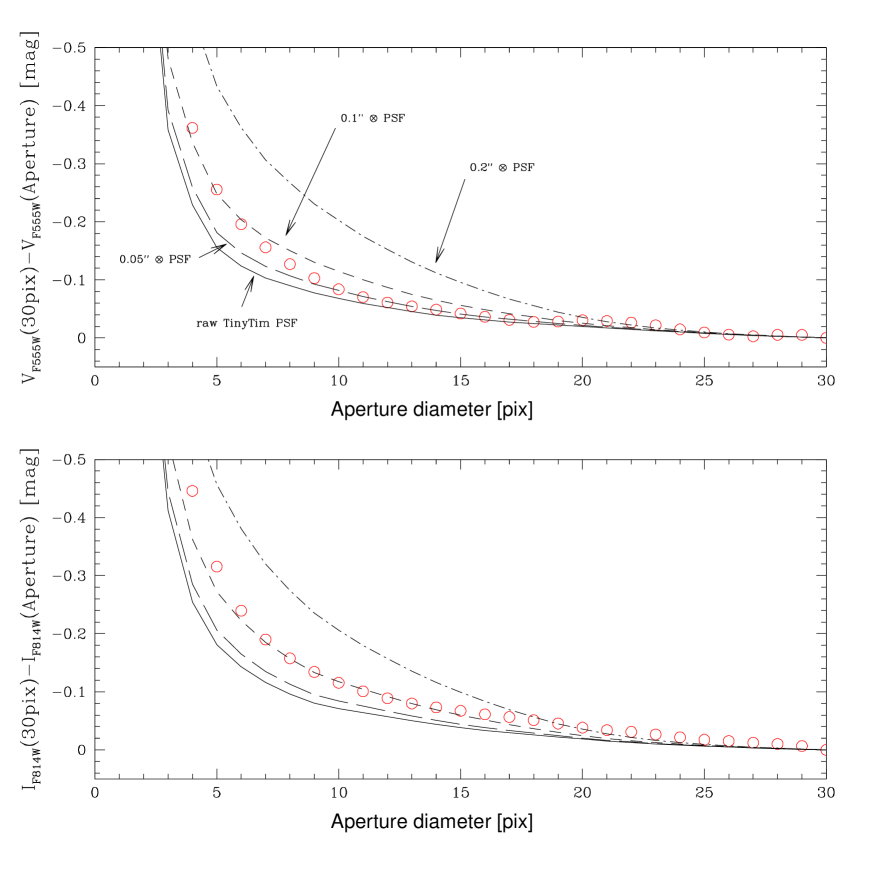
Figure 1: Curves of growth for PSF models and selected data. The curves represent different models (solid line = raw TinyTim PSF; long–dashed line = Hubble law (0.05 core radius) $\otimes$ PSF; short–dashed line = Hubble law (0.1 core radius) $\otimes$ PSF; dot–dashed line = Hubble law (0.2 core radius) $\otimes$ PSF while the open circles show the selected globular cluster data: 13 candidates in $V$ and 15 in $I$.

The modeled light profiles (see Fig. 1), unlike the real data, provide high enough signal–to–noise to determine the extrapolation from an 0.5 radius to the total $V$ and $I$ magnitudes. The derived corrections are applied to the 0.5 radius aperture measurements in addition to the Holtzman point source correction of $C=0.1$. These additional corrections are $C_{V}=0.050\pm 0.015$ and $C_{I}=0.080\pm 0.010$ (which results in a color correction of $C_{(V-I)}=0.030\pm 0.018$). The errors reflect the uncertainty in matching the data with the models and the accuracy of the extrapolation to infinity of our fit to the light profile. The errors do not include, for example, the fact that the core and the half–light radii of different globular clusters may vary significantly. In general, our data were calibrated applying the correction for point sources of $C=0.10$. When additional corrections were included, they are specifically mentioned in the text. Note that the corrections are systematic, i.e. they do not affect relative magnitudes. Therefore, the accuracy with which we are able to determine age–metallicity differences should not be seriously affected.

2.2.4 Artificial star/cluster experiments

Artificial star/cluster experiments were carried out using the tasks starlist and mkobjects from the IRAF package, artdata. 1000 objects were added per run in both the $V$ and $I$ images. 400 runs were computed resulting in 400,000 artificial objects per filter and covering the whole parameter space of background values. Both objects modeled by a WF chip PSF and objects modeled by the same PSF but convolved with Hubble laws of core radius 0.05 ($V$) and 0.1 ($I$) were added. All objects had a color of $V-I=1.1$, previous tests with 5000 objects having shown no significant variations among the completeness curves for $V-I=$ 0.9, 1.1 and 1.3.

The selection completeness was computed for objects found on both the $V$ and $I$ images. All detected objects which passed our selection criteria (see Sect. 2.2.5) and all input objects were sorted by their background value and subdivided in 10 background–value bins for $V$ and $I$, respectively. A skewed Fermi function

$$F(x)=\frac{ax+b}{1+\exp(x-c)^{d}}$$ (1)

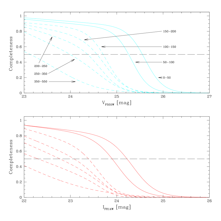
Figure 2: Completeness curves for the central pointing (dashed lines) and for the north– and south–pointings (solid lines). The central images have much higher background values than the northern and southern pointings. Each curve refers to a particular background value bin, i.e. from faint to bright magnitudes in counts: 0-50, 50-100, 150-200, 200-250, 250-350, 350-550.

was fit to all completeness histograms for each background bin. A smoothing procedure using a low–pass filter gives nearly the same results. The 50% completeness limits lie around $V\simeq 25.5$ and $I\simeq 24.5$ for the lowest background value. The 50% completeness magnitude falls off continuously with a growing background (see Fig. 2).

The artificial–object experiments also allowed us to determine the error in the photometry and to test the accuracy with which the FWHM of objects can be recovered as a function of magnitude. Typical FWHM values were deduced for extended objects which are a good match to the FWHM values of our globular cluster candidates.

2.2.5 Globular cluster selection criteria

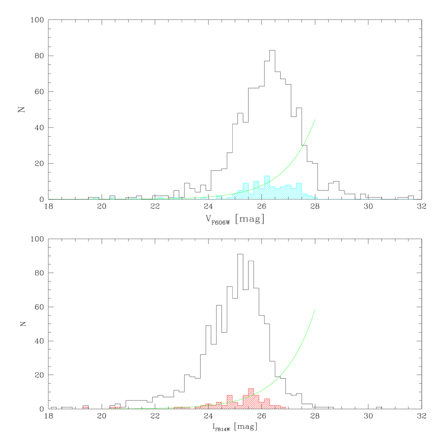
Figure 3: Background contamination histograms for the $V_{F606W}$ and $I_{F814W}$ band resulting from the HDF–N. The unshaded histograms show the background object luminosity distribution as obtained from HDF–N directly, while the shaded ones show the same data after applying our criteria. The lines are exponential least square fits to the small histograms. In order to ensure a reasonable fit we set the upper limit for the magnitude range at the 50% completeness level quantified during the completeness tests. Using the exponential law, the integrated number of background objects is $\sim 30$ up to the 50% completeness limit in both filters.

Object selection criteria were applied to our extracted data to provide a clean sample of globular cluster candidates for further analysis. Only objects which met the color cut of $0.5<V-I<1.8$ and a magnitude cut of $V\leq$ 25.5 and $I\leq$ 25.2 were included so that some of the red unresolved galaxy nuclei were rejected (cf. Fig. 3). In addition, a FWHM cut in the range 0.75 pix $<$ FWHM $<$ 2.5 pix was applied. We also calculated the magnitude difference obtained through apertures of 0.5 pix and 3 pix radii which allowed us to distinguish between point–source objects and extended objects like globular clusters (e.g. Schweizer et al. 1996). A very rough upper cut of $\Delta(0.5-3)>1.0$ was used.

The neural network of SExtractor v2.0.19, i.e. the $CLASS$ parameter was used to supplement the above selection criteria. This parameter was defined for well–sampled images (Bertin & Arnouts 1996). Since the WFPC2 provides under–sampled images the reliability of the $CLASS$ parameter is reduced. We applied only the selection criterion, $CLASS<1.0$, to our data. A test showed that for objects brighter than the 50% completeness level the $CLASS$ parameter cut reliably eliminates point sources and cosmic rays.

Our final list of globular cluster candidates includes 705 objects in $V$ and $I$. This is 38% of the initially extracted sample. An electronic list of the globular–cluster candidates is available from the authors.

2.2.6 Background contamination

One significant advantage of HST data over ground–based observations is high spatial resolution which allows high–confidence rejection of extended objects. However, background contamination is still expected. In order to determine the background fraction in our data we ran the same extraction and selection criteria for the Hubble Deep Field North (HDF–N, Williams et al. 1996) images. Since the HDF–N has galactic coordinates of $l=$ 125.89 and $b=$ +54.83 while our exposures have $l=$ 286.92 and $b=$ +70.20, we might overestimate the contamination due to foreground stars using this approach, although foreground star contamination is, in any case, expected to be negligible. We obtained from the HST Archive images in F606W and in the F814W filter with exposure times of 20200 sec for F814W and 15200 sec for F606W, respectively. These images are far deeper than our own. Both magnitudes for F606W and F814W were transformed to Johnson $V$ and Cousins $I$ magnitudes. We determined contamination histograms with and without the application of our selection criteria in order to establish their reliability. Exponential laws have been fit to the histograms, after applying the rejection criteria, up to the 50% completeness limits. The exponential laws act as input for our Improved Maximum–Likelihood Code (see Sect. 3.2.1).

Note the efficiency of our selection criteria. Nearly all background objects are removed from the data up to the 50% completeness magnitude. The contamination is less than 5% for both the $V_{F606W}$ and $I_{F814W}$ filters (see Fig. 3).

We stress again that all the above corrections were applied to the full sample, i.e. differential values between sub–samples remain unaffected even if small systematic effects have been introduced.

3 Analysis

Our goal is to determine the mean colors and turn–over magnitudes of the luminosity functions of the two main globular cluster sub–populations in both the $V$ and the $I$ filters. These colors and magnitudes can then be compared to the predictions of population synthesis models for given ages and metallicities.

3.1 Mean colors

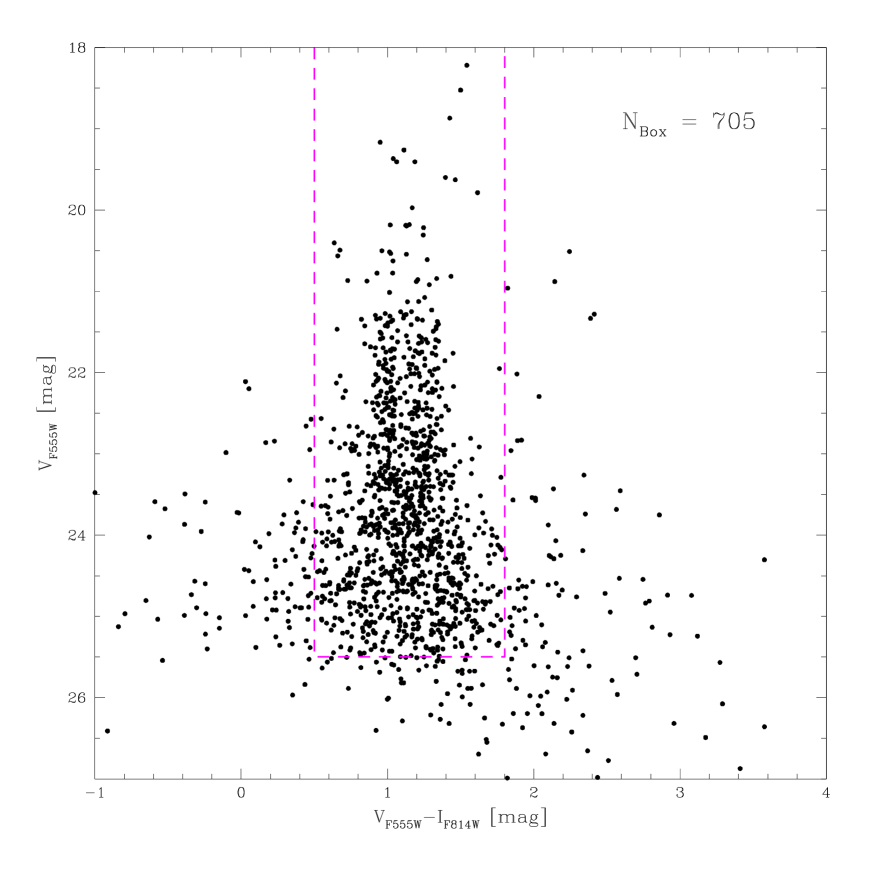
Figure 4: Color magnitude diagram of globular clusters in NGC 4472. The box delineates the initial cuts made to the raw data prior analysis. 705 globular cluster candidates are enclosed.

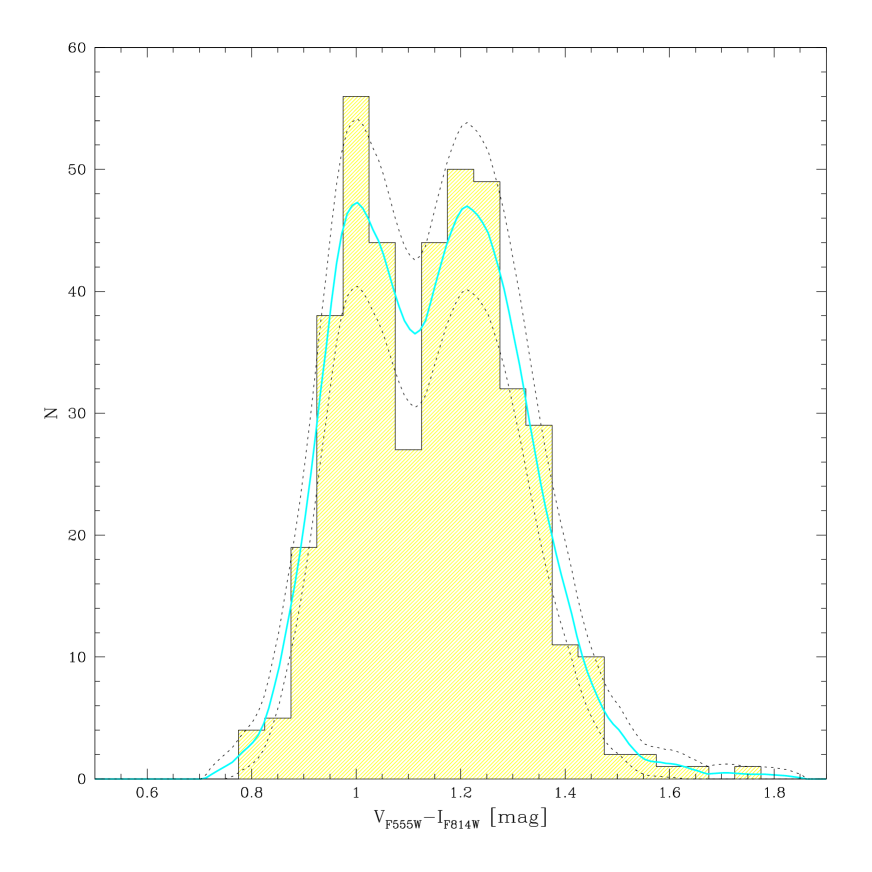
Figure 5: Color distribution of globular clusters in NGC 4472. A bimodal distribution is found to be present at the $99.99$% confidence level using the KMM mixture–modeling algorithm (Ashman et al. 1994). The two peaks lie at $0.99\pm 0.01$ and $1.24\pm 0.01$ ($0.93\pm 0.01$ and $1.18\pm 0.01$ corrected for reddening and aperture). A further analysis using a density estimation technique (kernel estimator with an Epanechnikov kernel) yields color peaks at $V-I=1.00\pm 0.01$ and $1.22\pm 0.01$. The solid line depicts the derived distribution function with statistical upper and lower error limits (short–dashed lines).

In order to determine the mean colors of the sub–populations we selected from the total sample objects with small photometric errors. The application of a magnitude cut at $V=23.75$ resulted in errors $\Delta(V-I)<0.05$. We further applied an upper magnitude cut at $V=20.0$ (corresponding to $M_{V}\simeq-11.2$ at the distance of Virgo) in order to exclude any foreground star contamination, and a broad cut in color ($0.8<(V-I)<1.8$) to isolate the region where globular clusters are expected. The color–magnitude diagram of our sample is shown in Fig. 4, together with the box (dotted lines) of pre–selected objects (see Sect. 2.2.5). A $(V-I)$ histogram of those selected objects is shown in Fig. 5.

Formally, a key underlying assumption is that the color (metallicity) does not significantly vary with magnitude (mass) within a sub–population. This appears to be the case as far as can be tested with our data.

A KMM test (Ashman, Bird & Zepf 1994) was run on our constrained sub–sample. The test determines the confidence with which bimodality can be said to be present, the most likely relative contribution of each population to the sample, and the peaks (i.e. mean colors) of each sub–population. We find that the color distribution is bimodal at the $>99.99$% confidence level. The relative contributions of objects to the selected sample (cf. Sect. 2.2.5) are 282 and 423 in the blue and red populations respectively. The peaks of the color distribution lie at $(V-I)=0.99\pm 0.01$ and $1.24\pm 0.01$ for the blue and red sub–populations, respectively. Formally, the peaks can be determined with an accuracy of 0.005 mag. The error adopted here reflects the range of values derived by varying the selection criteria (i.e. magnitude and color cuts).

Two fitting modes were used: 1) forcing identical dispersions (homoscedastic fit), 2) allowing independent dispersions (heteroscedastic fit). We note that substantially better fits, in terms of reduced $\chi^{2}$, are obtained if the dispersions of the blue and red distributions are allowed to differ, and that the red population seems to have a color distribution twice as broad as the blue one ($\sigma_{\rm blue}\simeq 0.06$, $\sigma_{\rm red}\simeq 0.12$).

We estimated the peak colors with yet another method that avoids the assumption of a Gaussian distribution for each color peak (intrinsic to the KMM code). We computed the density distribution in color of the objects with the help of a kernel estimator using the Epanechnikov kernel (e.g. Gebhardt & Kissler-Patig 1999). We used $h_{\rm opt}=0.043$ for the smoothing parameter (see Silverman 1986 for detailed discussion), an average of the optimal smoothing parameters for the blue and red peak ($h_{\rm opt}(\mbox{blue})=0.023$ and $h_{\rm opt}(\mbox{red})=0.063$) estimated from the $\sigma$–guess of KMM for both modes. The density distribution is overplotted in Fig. 5. A Biweight fit to each peak returns $(V-I)=1.00\pm 0.01$ and $1.22\pm 0.01$, in perfect agreement with the results from the KMM code.

To obtain the mean colors of the peaks, the above $(V-I)$ values need to be corrected for the calibration offset described in Sect. 2.2.3 ($\Delta(V-I)=0.030\pm 0.018$), and for a Galactic reddening towards NGC 4472 of E$(B-V)=0.0224$ (Schlegel et al. 1998), i.e. E$(V-I)=1.3\>\cdot\>{\rm E}(B-V)=0.029$ (following Dean et al. 1978). Note that the relative color difference, later used to derive the age difference, is only affected by these corrections in second order. The final, corrected mean colors of the two populations are $(V-I)_{0}=0.93\pm 0.02$ and $(V-I)_{0}=1.18\pm 0.02$.

3.2 Turn–over magnitudes

The TO magnitudes of the luminosity functions for the blue and red sub–population were individually determined in each filter using a Maximum Likelihood approach (cf. Secker 1992). The changing background counts over our whole sample motivated us to develop a version of Secker’s (1992) Maximum Likelihood Estimator which includes background variations. We calculated the completeness as a function of magnitude and background noise as described in Sect. 2.2.4. This improved code, described below, was used to derive the peak of the magnitude distribution for each filter and each sub–population.

Secker (1992) showed that the GCLF of the Milky Way and M31 was best represented analytically with the Student’s $t_{5}$-function

$$t_{5}(m|m_{o},\sigma_{t})=\frac{8}{3\sqrt{5}\pi\sigma_{t}}\left(1+\frac{(m-m_{o})^{2}}{5\sigma_{t}^{2}}\right)^{-3}.$$ (2)

We adopted the Student’s $t_{5}$–function as the most appropriate distribution for the GCLF of NGC 4472 since it matches the tails of the distribution better than a Gaussian function. The difference in the result using the one or the other function is, however, very small.

3.2.1 Improved Maximum Likelihood

Usually a dataset of $n$ independent observations, like a sample of magnitudes $M=(m_{1},m_{2},...,m_{n})$, is distributed in an unknown way. Assuming a distribution function $\phi(M|\Omega)$ which describes the distribution of data properly and depends on $q$ parameters $\Omega=(p_{1},p_{2},...,p_{q})$ (particularly the turn–over magnitude $m_{o}$ and the dispersion $\sigma_{t}$) the likelihood function $l(\Omega|M)=\phi(M|\Omega)$ is considered as a function $l$ of $\Omega$ for a given dataset $M$. The likelihood function is

$$l(\Omega|M)=\prod\limits_{i=1}^{n}\phi(m_{i}|\Omega).$$ (3)

For convenience, during the calculation the logarithmic likelihood function is used. During the evaluation the best set of parameters $\bar{\Omega}$ is found if

$$\frac{\partial l(\Omega)}{\partial\Omega}|_{\Omega=\bar{\Omega}}=0.$$ (4)

For a detailed treatment of Maximum Likelihood theory see, for instance, Bevington & Robinson (1992).

Our improved Maximum Likelihood code, based on Secker’s (1992) code, takes into account the influence of the background–noise level $\rho$ on the completeness function $I(m,\rho)$, in addition to the magnitude. Similarly, the photometric error function $\varepsilon(m,\rho)$ now also depends on these two variables. The distribution function is

$$\begin{array}[]{l}\phi(m|m_{o},\sigma_{t},\rho)=\\ \quad K\cdot\Phi(m|m_{o},\sigma_{t},\rho)+(1-K)\cdot B(m|\rho)\end{array}$$ (5)

where $m_{o}$ is the turn–over magnitude of the given distribution and $\sigma_{t}$ is its dispersion (note: $\sigma_{\rm Gauss}=1.291\cdot\sigma_{t_{5}}$), while $\rho$ is the background noise for the evaluation position on the chip. $K=N_{\rm GC}/(N_{\rm GC}+N_{\rm HDF})$ is the mixing parameter, i.e. the fraction of globular–cluster candidates in the whole data set including the background objects. Note that, in our case, K is close to 1.

It is necessary to normalize all the functions used, which is implicitly accomplished by

$$\begin{array}[]{l}\Phi(m|m_{o},\sigma_{t},\rho)=\\ \quad I(m|\rho)\cdot\left(\int t_{5}(m^{\prime}|m_{o},\sigma_{t})\cdot\varepsilon(m|m^{\prime},\sigma_{t})\,dm^{\prime}\right)\end{array}$$ (6)

and

$$B(m|\rho)=I(m|\rho)\cdot b(m)$$ (7)

where $b(m)$ is the background contamination function obtained from the HDF data. $\varepsilon$ is the photometric error function

$$\varepsilon(m|m^{\prime},\rho)=\frac{1}{\sqrt{2\pi}\cdot\sigma(m^{\prime},\rho)}\cdot\exp\left(\frac{(m-m^{\prime})^{2}}{2\cdot\sigma(m^{\prime},\rho)^{2}}\right)$$ (8)

which is assumed to introduce Gaussian errors to the distribution function $\phi$ with a magnitude and background noise dependent dispersion

$$\sigma(m,\rho)=\sqrt{10^{\>0.4\cdot(m-a)}+\rho^{2}\cdot 10^{\>0.8\cdot(m-b)}}.$$ (9)

The parameters $a$ and $b$ can be estimated with sufficient accuracy from a two–dimensional fit to the photometric errors obtained from the artificial star experiments. They act as input parameters to our code.

The need to account for the variable background, i.e. the need for the improved code, is best seen in Fig. 2. The selection completeness as a function of magnitude is plotted for a few typical values of background counts found in our datasets. The 50% completeness limits shift to brighter magnitudes with increasing background, i.e. photon noise.

Alternatively one could approximate a “mean” completeness by distributing the artificial stars with the same density profile as the globular clusters, without including the background as a parameter in the Maximum Likelihood analysis. The approach we have adopted is the more accurate solution to the problem. The package described above is available as an IRAF task from the authors.

3.2.2 Maximum Likelihood estimations

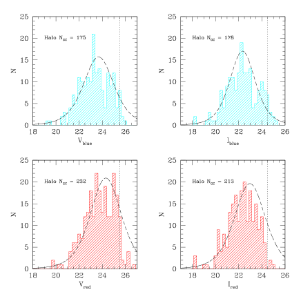
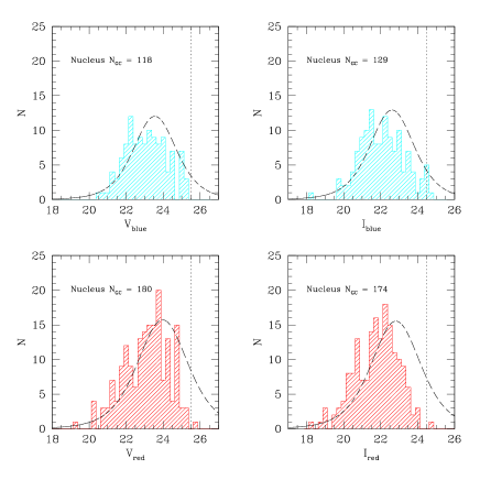
Figure 6: Globular cluster luminosity functions of the halo (Brodie) pointings (upper 4 plots) and central (Westphal) pointing (lower 4 plots). The number of clusters that went into the histograms up to the faintest completeness limit are indicated. The histograms are shown for the selected globular clusters, uncorrected for completeness and background variations (see text). The dashed curves are the best fitting $t_{5}$ functions as derived from our maximum–likelihood analysis, taking into account completeness and background corrections. The $t_{5}$ functions were arbitrarily normalized. The vertical dotted lines mark our 50% completeness limit at the lowest background value.

The Maximum–Likelihood routine of Drenkhahn (1999) was used to determine the TO magnitudes. Our completeness functions fit down to the 50% completeness levels ($V_{\rm faintest}\simeq 25.5$, $I_{\rm faintest}\simeq 24.5$) were used as the input. The data were convolved with the errors as a function of magnitude (see Eq. 6). The input globular cluster data were selected as described in Sect. 2.2.5. From KMM mixture modeling we determined that $(V-I)=1.1$ is the best value for separating blue and red clusters. For the analysis we split the full dataset into the central (Westphal) pointing and the combination of the halo (Brodie) pointings, since these two datasets had slightly different exposure times, i.e. slightly different limiting magnitudes/completenesses. The TO magnitudes for the individual pointings are given in Table 3, together with an average for the whole sample. The globular cluster luminosity functions are shown in Fig. 6. The values in Table 3 still need to be corrected for Galactic extinction ($A_{V}=0.069$ and $A_{I}=0.040$) and the additional aperture correction (see Sect. 2.2.3), however, these corrections do not affect the relative difference between the TO magnitudes.

We varied the input completeness and noise limits to the Maximum Likelihood code, the resulting TO magnitudes all lie within $<0.15$ mag.

As a consistency check, we attempted to reproduce the mean (uncorrected) colors of the sub–populations ($V-I$=0.99$\pm 0.01$ and 1.24$\pm 0.01$) by computing the differences between the $V$ and $I$ TO magnitudes for a given population. We obtained $(V-I)_{\rm TO}=1.14\pm 0.11$ for the blue population and $(V-I)_{\rm TO}=1.23\pm 0.16$ for the red population, where the errors are the errors of the $V$ and $I$ TOs taken in quadrature. The color for the blue population derived in this way is somewhat redder than that derived from the color distribution but the values agree to within the errors for both populations.

3.2.3 Monte–Carlo simulations

The error in the TO magnitude directly affects the error in the estimation of the age difference between the two sub–populations (see Sect. 4.1). We carried out Monte Carlo simulations to check whether our relatively modest sample sizes (which were as low as 118 to 232 objects when divided into inner and outer samples) affect the results significantly and to establish the associated error.

The blue and red samples were simulated in the $V$ filter using the number of objects in each sample and assuming a Gaussian distribution with the parameters derived above. These artificial samples were input into the Maximum–Likelihood code. The 68% confidence levels ($1\sigma$) on the TO magnitudes, from $10^{4}$ iterations, were 0.10 and 0.13 for the blue and red samples, respectively. These are in good agreement with the $1\sigma$ errors returned by the Maximum–Likelihood estimation.

3.3 Comparison with previous observations

The derived colors and TO magnitudes were compared to previous results from other groups.

3.3.1 The mean colors

Geisler et al. (1996) derived metallicity peaks for the blue and red sub–populations from Washington photometry. They found peaks at [Fe/H]$=-1.3\pm 0.38$ dex and $-0.1\pm 0.38$ dex for the blue and red sub–samples, respectively. Our colors, derived in Sect. 3.1, can also be translated into metallicities. However, large errors are introduced by the particular choice of a conversion relation of the $(V-I)$ color into metallicity. Using the relation given by Kissler-Patig et al. (1998a) ([Fe/H]$=-(4.50\pm 0.30)+(3.27\pm 0.32)\cdot(V-I)$), which is tuned to reflect the non-linear behavior at high metallicity, we obtain metallicities of [Fe/H]$=-1.45\pm 0.43$ dex and $-0.64\pm 0.49$ dex. These values are somewhat lower than, but within the errors of, the values derived by Geisler et al. (1996). Using the transformation of Kundu & Whitmore (1998), [Fe/H] $=-5.89+4.72\cdot(V-I)$, our data yield metallicities of [Fe/H] $=-1.50\pm 0.05$ dex and [Fe/H] $=-0.32\pm 0.05$ dex. The error corresponds to our photometric error in $(V-I)$ only. No calibration error of Kundu & Whitmore is considered. The metallicity calibration of Couture et al. (1990), [Fe/H] $=-6.096+5.05\cdot(V-I)$, gives the somewhat larger values of [Fe/H] $=-1.39\pm 0.05$ dex and $-0.11\pm 0.05$ dex, similar to those derived by Geisler et al. (1996).

3.3.2 The TO magnitudes

TO magnitudes have been derived by several groups but only for the whole sample (i.e. an average of the red and blue populations) and in different filters. Previous results should be compared to the average of our blue and red sample, with the necessary correction for reddening and aperture size: $V_{0}=23.76\pm 0.20$ (including the error on the TO magnitude and the error on the aperture correction). Furthermore, all other groups assumed E$(B-V)=0.00$ towards NGC 4472 (using Burstein & Heiles 1982/84) while we adopted the Schlegel et al. (1998) map from DIRBE/IRAS whose zero-point is offset by 0.020 in E$(B-V)$. Our value would translate into $V_{0}=23.83\pm 0.20$ if we assumed E$(B-V)=0.00$.

Using the Washington–Johnson transformation of Geisler (1996), $V\simeq T_{1}+0.5$, Lee et al.’s (1998) result translates into $V_{0}=23.81\pm 0.07$, in excellent agreement with our result. We note that Lee et al. investigated their blue and red samples separately, but did not find any significant difference in their TO magnitudes to within $\simeq$ 0.15 mag. However, their analysis was less rigorous in this respect than ours, and their data suffered from more background contamination, as is expected for ground–based observations.

Harris et al. (1991) derived $B_{TO}=24.78\pm 0.22$ with a 3–parameter Gaussian fit to the GCLF. Using $B-V\simeq 0.8$ for the total globular clusters population, this translates into $V_{TO}=23.98\pm 0.22$. Ajhar et al. (1994) derived $R_{TO}=23.3\pm 0.2$ (read off their Fig. 14) which, for $V-R\simeq 0.5$, translates into $V_{TO}=23.8\pm 0.2$. These results are in very good agreement with our determination.

3.4 Radial Dependencies

3.4.1 TO magnitudes as a function of radius

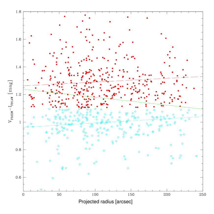
Figure 7: Radial distributions of the red (open circles) and blue (stars) globular clusters. The dashed line represents the best weighted linear least–square fit to the red population. The dot–dashed line gives the best fit to the blue population. The solid line shows the best fit for the entire globular cluster population. The gradient is twice as large as for each sub–population.

Variation in the TO magnitude with radius within a population can occur if the mean age, metallicity or mass changes with radius. Large age and metallicity gradients are ruled out by the absence of any significant color gradient in the sub–populations (see Fig. 7). A systematic change in the mean mass with radius could be caused by destruction processes shaping the globular cluster mass function. These are more important towards the center of the galaxy (e.g. recent work by Vesperini 1997 and Gnedin & Ostriker 1997), and significant changes are only expected within $\simeq 5$ kpc of the center ($\simeq 65$ at 16 Mpc). There the peak of the GCLF is expected to be brighter by up to $\simeq 0.3$ magnitudes, and the peak should be sharper as a consequence of the preferential destruction of low–mass clusters. Our inner sample (Westphal data) includes clusters at projected radii between 2 and 127 with a mean of 65  and our outer sample (Brodie data) includes clusters at projected radii between 76 and 252 with a mean of 160. Differences are therefore expected between these two samples. For the blue population, the TO magnitude varies from the inner to the outer regions by $0.12\pm 0.20$ and $-0.29\pm 0.25$ in $V$ and $I$ respectively. The weighted mean is $-0.04\pm 0.16$, i.e. we observed no brightening of the TO towards the center, although the uncertainty is on the order of the expected variation. For the red population the TO magnitude varies from the inner to the outer region by $0.33\pm 0.17$ and $0.14\pm 0.25$ in $V$ and $I$ respectively. Formally, the TO appears brighter by $0.27\pm 0.14$ (weighted mean) for the inner red population. We do not see any changes in the dispersion of the GCLF to within the errors.

This result is probably not yet secure enough to be worth commenting on in depth. However, a difference between the red and blue population could occur, for example, if the blue and red clusters are on different orbits. Sharples et al. (1998) found tentative evidence for the blue clusters in NGC 4472 having a higher velocity dispersion and higher rotation than the red ones. Kissler-Patig & Gebhardt (1998) found a similar (but firmer) result for M 87, another giant elliptical that hosts enough globular clusters for such an analysis. If indeed the blue clusters are preferentially on tangential orbits, while the red clusters are preferentially on radial orbits, destruction processes would be more efficient for the red population.

Finally, we note that Harris et al. (1998) and Kundu et al. (1999) also looked for this effect in M 87. Kundu at al. even looked for trends in the blue and red populations separately. Neither group found any brighting of the GCLF towards the center of M 87, but note again that the uncertainties in the measurements are still of the order of the expected signal.

3.4.2 Color as a function of radius

We looked for color gradients within the sub–populations using a weighted least squares fitting routine. In addition to the color cuts ($0.5<V-I<1.1$ and $1.1<V-I<1.8$), the samples were cut at $V$ = 24.8 to provide at least 50% completeness even in the central regions. The results are plotted in Fig. 7, together with a fit for the total sample. The derived gradients are $\Delta(V-I)/\Delta\log r=0.015\pm 0.004$ mag/log(arcsec) and $0.013\pm 0.007$ mag/log(arcsec) for the blue and red population respectively. Different color and magnitude cuts scatter these results within 0.01 mag/log(arcsec). Any positive gradients in the sub–populations are either very small or non–existent. For the whole sample, however, we find a clear negative gradient of $\Delta(V-I)/\Delta\log r=-0.029\pm 0.07$ mag/log(arcsec), corresponding to a metallicity gradient of $\Delta$[Fe/H]$/\Delta\log r\simeq-0.15\pm 0.02$ dex/log(arcsec) (somewhat dependent on the color–metallicity relation used).

We confirm Geisler et al.’s (1996) result, that this gradient is caused by the changing ratio of red to blue clusters as a function of radius, rather than an overall decrease in metallicity with radius. Quantitatively, we find a somewhat smaller gradient than reported by Geisler et al. (1996), who found $\Delta$[Fe/H]$/\Delta\log r\simeq-0.4$ dex/log(arcsec). This is probably due to our smaller radial coverage and our use of a less metallicity–sensitive color. Indeed, our sample extends to only 250 while Geisler et al.’s data extend out to $\simeq$ 500. The ratio of blue to red clusters varies by only $\simeq$ 10% from our inner to outer regions, as derived from a comparison of their cumulative radial distributions.

A similar situation is seen in M 87, for which Harris et al. (1998) report no color gradient within 60, and Kundu et al. (1999) report a weak gradient of $\Delta(V-I)/\Delta\log r=-0.017\pm 0.012$ mag/log(arcsec) within 100. However, Lee & Geisler (1993) report a strong gradient ($\Delta$[Fe/H]$/\Delta\log r=-0.65\pm 0.17$ dex/log(arcsec)) over 500 radius.

3.5 Globular Cluster Sizes

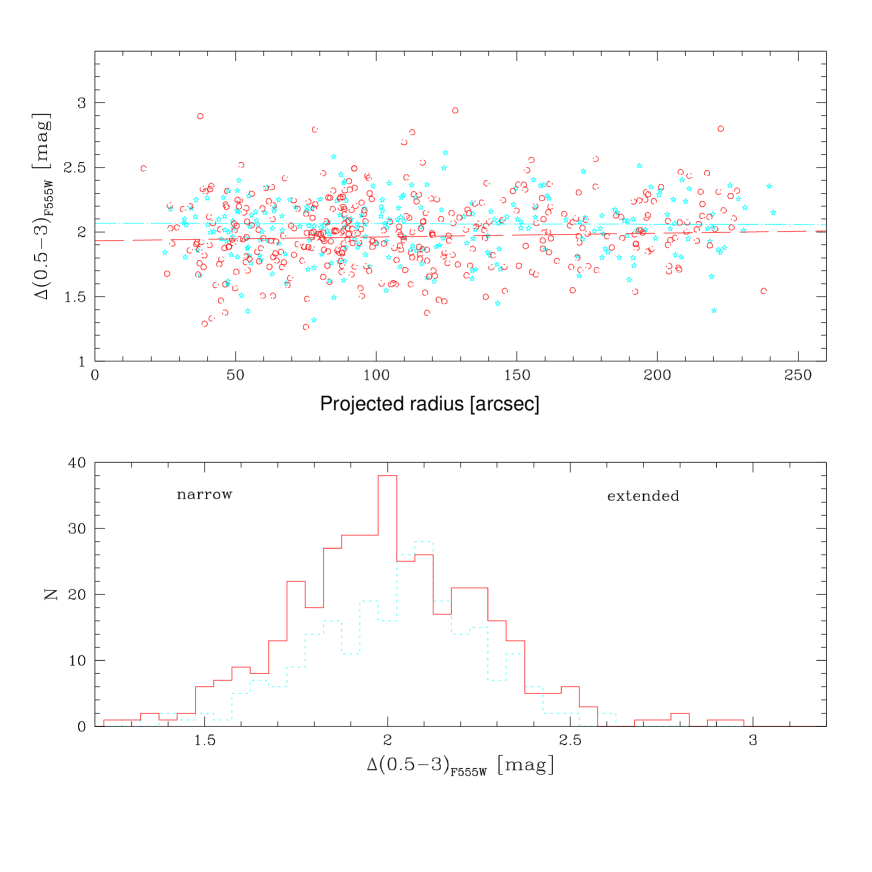
Figure 8: Upper panel: Radial globular cluster size distribution for blue (open stars) and red (open circles) globular clusters. The dot–dashed line is the best least–square fit to the blue sub–population while the dashed line gives the best fit to the red sub–population. Lower panel: Histogram of relative globular cluster sizes for the red population (solid histogram) and the blue population (dashed histogram). The sizes of the blue globular clusters are substantially larger than those of the red.

The high resolution of HST allows us to study the relative sizes (see Sect. 2.2.3) of the globular cluster candidates using the parameter $\Delta(0.5-3)$ (see Sect. 2.2.5). For extended objects the magnitude difference in two different apertures will appear large as the light profile contributes a non–negligible amount of light to the outer aperture. The opposite is the case if the light profile is narrow. For this analysis, we restricted ourselves to clusters found on the Wide Field (WF) camera chips, to avoid the problematic conversion between the WF and the Planetary Camera (PC). Fig. 8 presents the histogram of globular cluster sizes for both the blue and red sub–populations. The median values for these two distributions point to a systematic size difference between the blue and the red globular clusters. The median values for the blue and red populations are $m_{\Delta}=2.06\pm 0.01$ mag and $m_{\Delta}=2.02\pm 0.01$ mag, respectively, indicating that the blue globular clusters are substantially larger than the red globular clusters. A Maximum–Likelihood estimation of the mean and its error yields the same results.

Interestingly, in both NGC 3115 (Kundu & Whitmore 1998) and M 87 (Kundu et al. 1999), the blue clusters also appear significantly larger than the red ones. The authors suggest this is due to different radial distributions for the red and blue clusters, noting that Galactic globular clusters with larger galactocentric distances have larger half–light radii (van den Bergh 1994).

To study the radial dependence of globular cluster size, we plotted the size parameter ($\Delta(0.5-3)$) versus radius and found no gradients: $\Delta(0.5-3)=2.07(\pm 0.03)-0.5(\pm 3.2)\cdot 10^{-4}\cdot r$ where $r$ is the radius in arcsec, and $\Delta(0.5-3)=1.93(\pm 0.03)-2.9(\pm 2.7)\cdot 10^{-4}\cdot r$, for the blue and red clusters respectively (see also Fig. 8). The difference between blue and red clusters is present at all radii. We therefore speculate that the different sizes are a relic of the different formation processes, unless the red and blue clusters are on significantly different orbits. For example, the red clusters could be preferentially on radial orbits and be systematically more affected than the blue clusters by the central potential during their close passage near the galaxy center.

4 The age difference between the main sub–populations

4.1 Comparison with the models

We compare our results (TO magnitude and mean color) to various population synthesis models in order to derive the age difference between the blue and red globular cluster sub–populations.

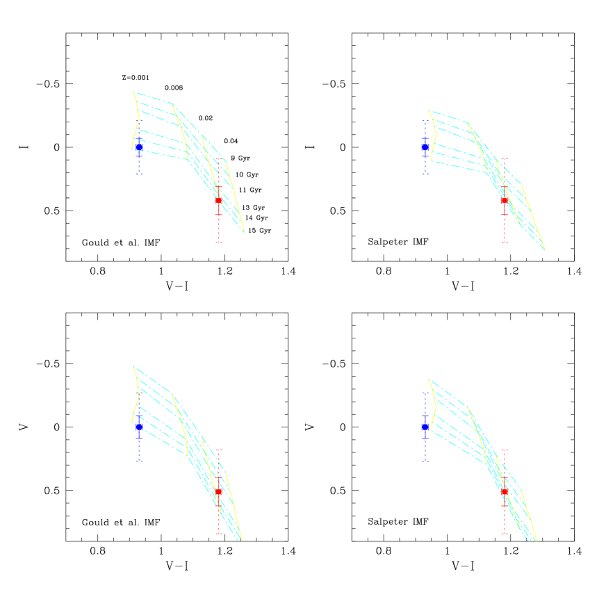
Figure 9: Maraston’s (1998) Simple Stellar Population models. Upper panels: I–band data. Lower panels: V–band data. The solid grid lines represent iso–metallicity tracks of $Z$ = 0.001, 0.006, 0.02, 0.04. Dash–dotted lines are isochrones of 9, 10, 11, 13, 14 and 15 Gyr. Solid error bars represent 1$\sigma$ errors and dashed error bars refer to 3$\sigma$ errors. The averaged maximum age difference (age${}_{\rm blue}-$ age_red) is $\Delta T=0.7\pm 1.8$ Gyr.

We used the new models from Maraston (1998) as well as the most recent models from the Göttingen Group (Kurth et al. 1999), and the models from Bruzual & Charlot (1996) and Worthey (1994). In each case we compared our data to every available Initial Mass Function (IMF), i.e. usually the Salpeter IMF and a multi–slope IMF. The full range of metallicities was used as well as the necessary age range. Since we are only interested in age differences the exact normalization of the absolute magnitude, which is dependent on mass and mass–to–light (M/L) ratio for a given IMF, is not important. The grids in Fig. 9 to 12 can, therefore, be somewhat arbitrarily shifted in the y–direction. In the following, we fixed the grids in the y–direction such that the oldest sub–population lies on the oldest computed isochrone (15 Gyr or 16 Gyr). Further, we arbitrarily set the blue population to $V=0$ and $I=0$ in order to compare the different models directly. There is no freedom in the x–direction since the color is not mass–dependent, and the grid is fixed in $V-I$ for a given stellar population.

For the mean colors of the blue and red sub–populations we used the colors derived in Section 3.1. The TO values used were the ones derived for the full sample (see Table 6). We stress again that additive corrections to both the blue and red TO magnitudes (i.e. reddening correction, potential systematic errors, aperture corrections) only influence the difference as second order effects, if at all, and are not a concern.

However, we make two important underlying assumptions. We assume that the M/L ratios for blue and red clusters are only dependent on age and metallicity (i.e. the IMFs of the blue and red clusters are similar). Second, we assume that blue and red cluster populations have the same underlying mass distribution (by which we mean globular cluster masses, not IMFs). Under these assumptions, TO magnitudes are influenced only by age and metallicity. We briefly discuss the validity of these assumptions and the errors they potentially introduce.

4.1.1 The M/L and mass distribution assumptions

Kissler-Patig et al. (1998b) review the empirical reasons for expecting the mass distributions and M/L ratios to be similar among various sub–populations. Briefly, the M/L assumption is essentially the assumption that both blue and red clusters have similar IMFs, at least below 1 $M_{\odot}$ where it influences our result. Observations so far for globular clusters in the Local Group seem to confirm this picture (e.g. Dubath & Grillmair 1997). In the case of the mass distribution, globular cluster formation seems to follow a universal mechanism (e.g. Elmegreen & Efremov 1997). The constancy of the TO magnitude from galaxy to galaxy (e.g. the review by Whitmore 1997) and the observed mass distributions of young clusters (e.g. brief review by Schweizer 1997) support this picture.

The possibility that size differences might indicate different formation processes for blue and red clusters was discussed in Section 3.5. It is not clear, however, whether it is only the mean sizes or also the mean masses that are affected. Moreover, our assumption would fail if, despite similar mass distributions at formation, blue and red clusters are affected differently by destruction processes. There is a hint (see Section 3.4) that this might be the case in the inner region, where the difference between the blue and the red TO magnitudes is smaller by $0.32\pm 0.24$ (combining the $V$ and $I$ information) than in the outer region. (We note for completeness that an age gradient in the population would have the same observable effect as a mass gradient). If this effect is real, the TO difference of the total sample, as used, could be affected by a 0.1 to 0.2 mag systematic error. We estimate that this empirical determination gives about the right order of magnitude for the potential systematic error in our method and, in what follows, we will assume a potential systematic error of $\simeq 0.2$ mag, which translates into roughly 4 Gyr.

Note that for similar M/L values of the blue and red clusters, such a difference of 0.2 mag would translate into only a 20% difference in the mass characterizing the TO. Irrespective of the accuracy needed for our study, blue and red clusters have roughly similar mass distributions.

4.1.2 Avoiding assumptions about the masses

For completeness, we mention a method for checking the validity of these assumptions and a method for avoiding them.

For the chosen filters, age and characteristic mass influence the TO far more than metallicity, which is fairly well determined by the color. Therefore, one could determine the mean mass difference (and check the above assumption) by obtaining an independent estimate of the mean age difference. An independent age estimate could be obtained with spectroscopy of a large number of globular clusters and the measurement of an age–sensitive absorption line index. Several tens of H$\beta$ measurements in each sub–population would allow the mean H$\beta$ value to be determined to within $<0.1$ Å which would translate into an accuracy in the mean age difference of $\simeq 2$ Gyr. This in turn would allow us to verify that the characteristic TO masses of the red and blue populations lie within 10% to 20% of each other.

An alternative method for determining the mean age difference without making any assumptions about the mass distributions would be to use mass–independent quantities that depend only on age and metallicity. Broad–band colors are such quantities. A plot similar to Figures 9 through 12, but in a color–color plane, would remove any uncertainties due to different mass distributions. However, it is impossible to find two colors in the optical and NIR spectrum that disentangle age and metallicity as efficiently as the color/TO magnitude combination.

4.1.3 Comparison with Maraston (1998)

In Figure 9, we compare our results to the models of Maraston (1998). She computed single burst population models with a Salpeter (1955) and multi-slope IMF (Gould et al. 1998) for metallicities Z$=0.001,0.006,0.02$ and $0.04$, and ages up to 15 Gyr. We refer the reader to the original paper for further details of the modeling.

The derived age difference, which is quoted in the following as (age_blue)$-$(age_red), varies between $\sim-0.3$ Gyr (Gould et al. IMF, $I$ band) and $\sim+2.4$ Gyr (Gould et al. IMF, $V$ band), with errors of about 2.7 Gyr (1$\sigma$). Within the errors, the blue and red population appear coeval, with a formal difference of $+0.7\pm 1.8$ Gyr (straight mean of the four computed differences with their dispersion shown as the error). A 3$\sigma$ limit on the age difference would be around 6 Gyr.

4.1.4 Comparison with Kurth et al. (1999)

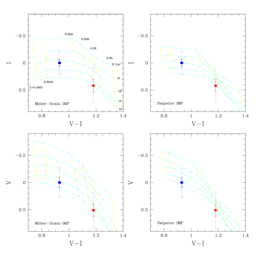
Figure 10: Simple Stellar Population models by Kurth et al. (1999) calculated for a single stellar burst of $10^{7}$ Gyr duration. Upper panels: I–band TO magnitudes. Lower panels: V–band TO magnitudes. Within the grids the solid lines (vertical) represent iso–metallicity tracks of $Z$ = 0.0001, 0.0004, 0.004, 0.008, 0.02, 0.05 (from left to right) which correspond to [Fe/H]$=-2.3,-1.7,-0.7,-0.4,$ 0.0 and 0.4. The dash–dotted (horizontal) lines are isochrones of 8, 10, 12, 14 and 16 Gyr. The solid error bars represent the 1$\sigma$ errors. The dotted error bars give the 3$\sigma$ deviations. An averaged maximum age difference of $\Delta T=-2.3\pm 1.6$ Gyr is derived.

In Figure 10, we compare our results to the recent models of Kurth et al. (1999). They computed single burst models with a Salpeter (1955) and a Miller–Scalo (1979) IMF for 6 metallicities between Z$=0.0001$ and $0.05$, and ages up to 16 Gyr.

The age difference varies between $-3.8$ Gyr (Salpeter IMF, $I$ band) and $-0.4$ Gyr (Salpeter IMF, $V$ band) with a typical error of 2.2 Gyr. The mean difference is $-2.3\pm 1.6$ Gyr, i.e. the red population appears somewhat older than the blue one. The 3$\sigma$ differences are around $-7$ and $+2.5$ Gyr.

4.1.5 Comparison with Bruzual & Charlot (1996)

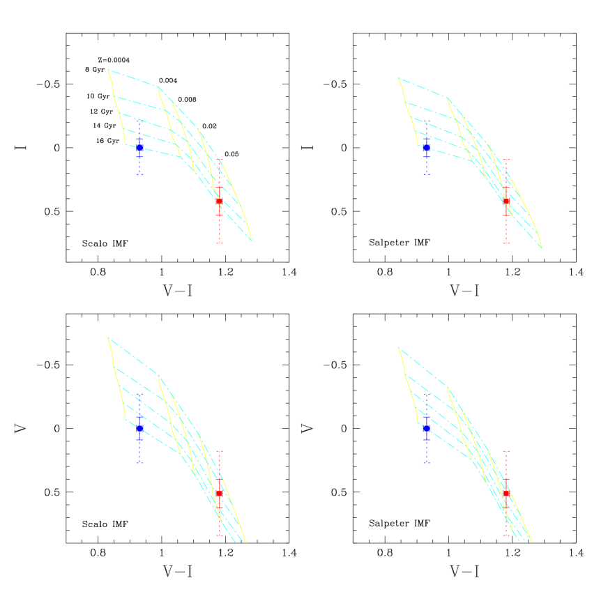
Figure 11: Simple Stellar Population models by Bruzual & Charlot (1996). Upper panels: I–band data. Lower panels: V–band data. The solid grid lines represent iso–metallicity tracks of $Z$ = 0.0004, 0.004, 0.008, 0.02 and 0.05. Dash–dotted lines are isochrones of 8, 10, 12, 14, 16 Gyr. Using these grids an averaged maximum–age difference of $\Delta T=3.3\pm 2.2$ Gyr was derived.

In Figure 11, we compare our results to the models of Bruzual & Charlot (1996). We used the single burst populations computed with a Salpeter (1955) IMF and a Scalo (1986) IMF, with metallicities between Z$=0.0004$ and $0.05$. Their models with a Miller–Scalo (1979) IMF were not used. The tracks for their highest metallicity (Z$=0.1$) are not shown. The oldest modeled populations is 16 Gyr.

The age differences vary between $+1$ Gyr (Scalo IMF, $I$ band) and $+6$ Gyr (Salpeter IMF, $V$ band), with an typical error of 2.8 Gyr. The mean difference is $+3.3\pm 2.2$ Gyr. The 3$\sigma$ limits lie around $-3$ and $+10$ Gyr.

4.1.6 Comparison with Worthey (1994)

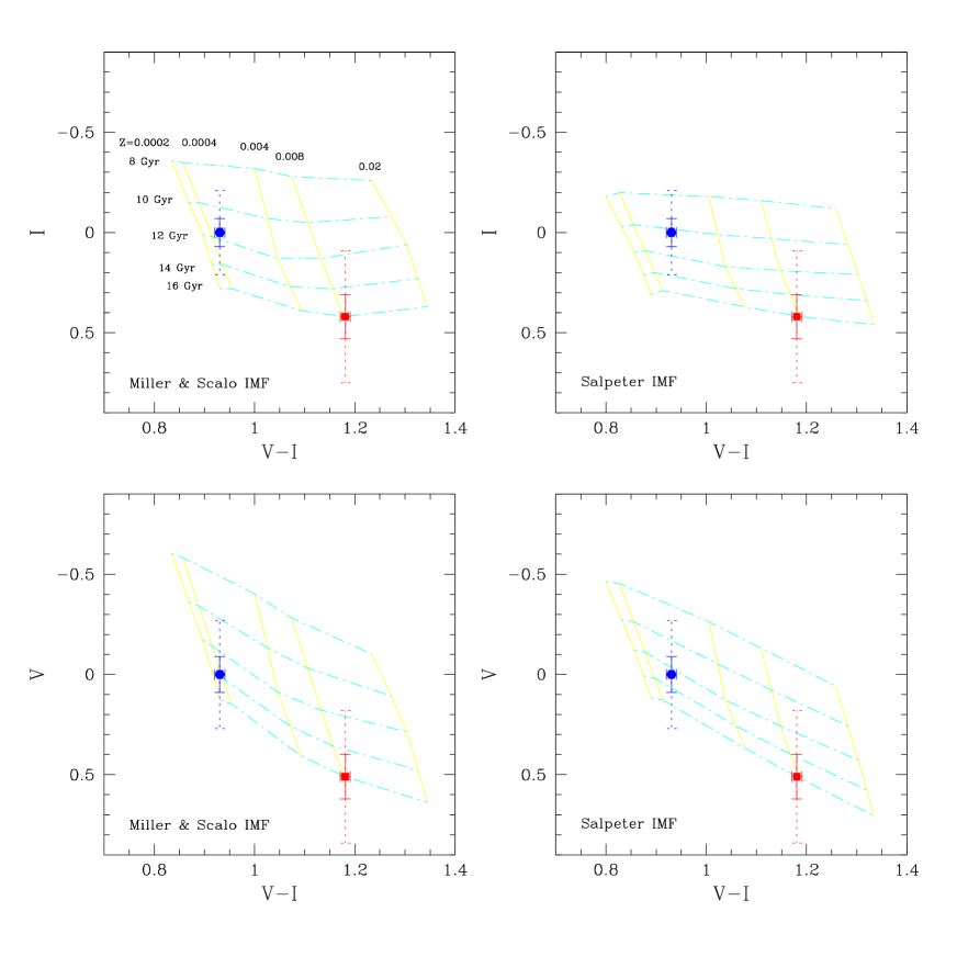
Figure 12: Worthey’s (1994) Simple Stellar Population models. Upper panels: I-band data. Lower panels: V-band data. The solid grid lines represent iso–metallicity tracks of $Z$ = 0.0002, 0.0004, 0.004, 0.008, and 0.02. Dash–dotted lines are isochrones of 8, 10, 12, 14, 16 Gyr. The averaged maximum age difference is $\Delta T=-4.0\pm 1.6$ Gyr.

In Figure 12, we compare our results to Worthey’s (1994) single burst models. He computed models with a Salpeter (1955) IMF and a Miller–Scalo (1985) IMF for metallicities between Z$=0.0002$ and 0.05, up to an age of 16 Gyr.

The age difference varies between $-5.8$ Gyr (Salpeter IMF, $I$ band) and $-2.1$ Gyr (Miller–Scalo IMF, $V$ band), with a typical error of 2.5 Gyr. The mean difference is $-4.0\pm 1.6$ Gyr, i.e. the red populations appears older than the blue one. The 3$\sigma$ limits are around $-9$ and $+1$ Gyr.

4.1.7 The maximum age difference between the globular cluster populations

We note that the $I$ band results give a systematically smaller difference (in the sense we defined it: age${}_{\rm blue}-$age_red) than the $V$ band results. Except for the Bruzual & Charlot (1996) models, the results from the $I$ band suggest that the red population is marginally older than the blue one.

The different models predict mean differences anywhere between $-4.0$ Gyr and $+3.3$ Gyr, with a mean of $-0.6$ Gyr and a dispersion of $3.2$ Gyr. It would be somewhat arbitrary to assign more weight to one model than to another, so that we are currently limited in the age determination by the model uncertainties. Nevertheless, it seems that both populations are coeval within the errors, and we can exclude at the 99% confidence level one population being half as old as the other.

If our results are affected by a systematic error, e.g. if the smaller sizes of the red globular clusters do indeed translate into a lower “mean” mass (such that the red TO magnitude is $\simeq 0.2$ lower – see Section 4.1.1), the age difference would be affected by $\simeq+4$ Gyr.

4.2 Implications for the star formation episodes of NGC 4472

The above results suggest that the vast majority of globular clusters and stars formed at high redshift in this cluster galaxy. As already mentioned in Section 1, several other lines of evidence lead to similar results for cluster galaxies. Interestingly, the globular cluster results imply that two major star–formation events took place at high redshift. Those two events appear to have happened moderately closely in time but from differently enriched gas. The blue clusters appear to have formed from gas with less than $1/20$th solar metallicity while the red clusters formed out of gas with close to solar metallicity. Furthermore, the mean sizes of the blue and red clusters appear to be significantly different. This suggests different conditions at the formation epoch, unless they are directly related to the metallicity and associated cooling processes in the molecular clouds in which the clusters originated.

It is unclear whether the blue or the red clusters are the older ones. At face value it seems odd that the more metal–rich clusters would be the older ones. However, in scenarios where the blue clusters formed in halo clouds (e.g. Kissler-Patig et al. 1998b) or were accreted with dwarf galaxies (e.g. Côté et al. 1998, Hilker et al. 1999a,b), this could be understood in terms of the large structures (e.g. bulges) collapsing first, followed shortly thereafter by the smaller structures (clouds/dwarf galaxies). This, however, would force a revision of the merger scenario which clearly predicts that the red clusters will be younger than the blue ones.

Alternatively, if two sub–populations of clusters are coeval or if the blue clusters are the older ones, age differences of a few Gyr between the different sub–populations could be explained in all globular cluster/galaxy formation scenarios, i.e. the above–mentioned scenarios, merging (Ashman & Zepf 1992), or in–situ formation of distinct populations (e.g. Forbes et al. 1997, Harris et al. 1998, Harris et al. 1999). We note only that, in the merger scenario, merging would have to have taken place at early times ($z>1$ at the 3$\sigma$ level) which is somewhat at odds with the recent theoretical predictions from hierarchical clustering models (e.g. Kauffmann 1996, Baugh et al. 1998). These tend to predict that the main star formation in cluster environments occurred at redshifts $z<1$.

5 A distance estimation for NGC 4472

The TO magnitude ($V_{TO}$) of the GCLF appears to be essentially universal and, therefore, can be used as a distance indicator (e.g. the review by Whitmore, 1997). $V_{TO}$ depends on the age and metallicity of the globular clusters (Ashman, Conti & Zepf 1995, see also Sect. 4.1), and weakly on galaxy type (Harris 1997) which may be a consequence of the age/metallicity dependence. The derived TO magnitude for the globular clusters in NGC 4472 can be used to obtain a distance to the galaxy.

5.1 The absolute turn–over magnitude

The method is best calibrated using the TO magnitude of the Milky Way GCLF, since it involves the minimum number of steps on the distance ladder. The M31 GCLF serves as a strong check on this calibration (cf. Ferrarese et al. 2000; Kavelaars et al. 1999).

The Milky Way system is dominated by old globular clusters of mean metallicity [Fe/H]$\simeq-1.4$. It is, therefore, well–suited to fitting the TO magnitude of the blue population in NGC 4472 (see Sect. 4.1) and no correction for age–metallicity dependence need be applied. However, we have to assume that age–metallicity dominates any dependence on galaxy type, and that globular cluster mass functions are intrinsically similar, which seems justified to first order (e.g. Kissler-Patig et al. 1998b).

Della Valle et al. (1998) recently re–derived $V_{TO}$ for the Milky Way system. To derive individual distances to all Galactic globular clusters, they adopted a horizontal branch (HB) magnitude – metallicity relation derived from globular cluster main sequence fitting using distance measurements to sub–dwarfs from HIPPARCOS (in this case by Gratton et al. 1997). From the resulting GCLF they obtained $V_{TO}=-7.62\pm 0.06$ noting that, depending on the adopted HB magnitude–metallicity relation, this result could suffer from a 0 to $-0.2$ mag systematic error.

Drenkhahn & Richtler (1999) used a different approach. They assumed the LMC distance to be the fundamental zero–point (here $(m-M)=18.46\pm 0.06$), and derived an RR Lyrae magnitude–metallicity relation. The remaining steps were similar to those of Della Valle et al.. Drenkhahn & Richtler found $V_{TO}=-7.61\pm 0.08$ and $I_{TO}=-8.48\pm 0.10$ for the Milky Way GCLF.

5.2 The distance to NGC 4472

The apparent TO magnitude derived for the blue population is $V_{TO}=23.62\pm 0.09$ and $I_{TO}=22.48\pm 0.07$ (see Tab. 6). These values need to be corrected for the photometric term discussed in Sect. 2.2.3 ($\Delta C_{V}=0.050\pm 0.015$, $\Delta C_{I}=0.080\pm 0.010$), as well as for Galactic extinction ($A_{V}=0.069$, $A_{I}=0.040$). Using the absolute TO magnitudes discussed above, we derive distance moduli of $(m-M)_{V}=31.11\pm 0.19$ and $(m-M)_{I}=30.84\pm 0.14$ (adding all errors in quadrature), i.e. a mean $(m-M)=30.99\pm 0.11$ (where the error does not include any possible systematic error in the calibration). The corresponding distance is $15.8\pm 0.8$ Mpc.

A quick comparison with distances derived for NGC 4472 by other methods shows very good agreement (despite completely different calibrations). Jacoby et al. (1990) derived $(m-M)=30.84\pm 0.11$ from the planetary nebulae luminosity function. Tonry et al. (1990) and Neilsen (1999) derived $(m-M)=30.78\pm 0.07$ and $(m-M)=30.93\pm 0.08$, respectively, from surface brightness fluctuations.

Cepheid distances now exist for 7 spiral galaxies in the Virgo Cluster (cf. Pierce et al. 1994 and Ferrarese et al. 2000). With the exception of NGC 4639 (Saha et al. 1996), which appears to be background to the main body of spirals, the mean distance to the other 6 galaxies is $(m-M)=31.01\pm 0.07$ or 16.0$\pm$0.6 Mpc. Our GCLF distance to NGC 4472 is in excellent agreement with this distance, which supports the view that the Virgo cluster spirals and ellipticals are at essentially the same distance.

6 Summary

The age difference between the two major globular cluster sub–populations in an early–type galaxy has been determined. We have developed an age differentiating method which uses the precise TO magnitudes and colors of the sub–populations. We have applied this method to NGC 4472, matching our observables to several SSP synthesis models.

An extended–object analysis showed that at the distance of Virgo (i.e. $\sim$16 Mpc) HST is capable of resolving single globular clusters. Thus it is necessary to make an additive correction (of $C_{V}=0.050\pm 0.015$ mag and $C_{I}=0.080\pm 0.010$ mag at the distance of Virgo) to the mean correction of $C=0.1$ mag (for point sources) when extrapolating HST photometry obtained in 0.5 radius apertures to total luminosities. This corresponds to a color correction of $C_{(V-I)}=0.03\pm 0.018$.

We found the globular cluster color distribution in NGC 4472 to be clearly bimodal (at the 99.99% confidence level) with two peaks located at $V-I=0.99\pm 0.01$ and $1.24\pm 0.01$ corresponding to $(V-I)_{0}=0.93\pm 0.02$ and $(V-I)_{0}=1.18\pm 0.02$ when corrected for reddening and finite aperture. We determined that the red globular clusters have a color distribution almost twice as broad as the blue ones.

We divided the whole globular cluster population into an inner and an outer sample, as defined by the HST different pointings. We used an improved Maximum–Likelihood estimator, which accounts for varying background values, to determine the TO magnitudes for each sub–population in each radial sample (see Tab. 6). The TO of the blue sub–population is the same for the inner and outer sample. By contrast, the red sub–population appears to be marginally brighter by $0.27\pm 0.14$ mag in the inner region than in the outer region. This difference is of the expected order of magnitude if destruction processes act on the red sample within 5 kpc.

The radial color distributions of each sub–population show almost no gradients. However, we detected an overall gradient of $\Delta(V-I)/\Delta\log r=-0.029\pm 0.07$ mag/log(arcsec) in the system, which is mostly an effect of the changing ratio of red to blue globular clusters with radius (cf. Geisler et al. 1996).

Taking advantage of HST’s high spatial resolution, we estimated the mean sizes of the globular clusters using the $\Delta(0.5-3)$ parameter. The blue globular clusters were found to be larger than the red ones, as was already observed in M 87 (Kundu et al. 1998) and NGC 3115 (Kundu & Whitmore 1997). The most likely explanations are that the size difference reflects different formation processes, or that red clusters are on preferentially radial orbits, while blue clusters are on preferentially tangential orbits.

We used 4 different SSP models to derive the mean age difference between the red and blue sub–population. Our underlying assumption was that both blue and red populations have similar mass distributions which appears to be valid at least at the 10% to 20% level (which, nevertheless, corresponds to a potential systematic error of $\sim 4$ Gyr). The mean age difference between the blue (metal–poor) and the red (metal–rich) sub–populations is age${}_{blue}-$ age${}_{red}=-0.6\pm 3.2$ Gyr, where the error is the dispersion introduced by the different models (for a given model the error on our method is $\sim$2 Gyr).

We conclude that the globular clusters (and by association the stars) in NGC 4472 formed in two major episodes/mechanisms that were coeval within a few Gyr.

The images as well as electronic lists of the photometry are available from the authors. Also available is the maximum–likelihood code as an IRAF task used to derive the globular cluster luminosity functions taking into account the background variations over the field.

Acknowledgments

We are very thankful to Claudia Maraston for customizing part of her models for our purposes and providing electronic files, as well as to Georg Drenkhahn for his help in implementing his Maximum Likelihood code. We also thank Sandy Faber, Duncan Forbes, Karl Gebhardt, and Klaas de Boer for interesting discussions.

THP gratefully acknowledges support from the UCO/LICK Observatory. MKP was partly supported by the Alexander von Humboldt Foundation. This research was funded by HST grants GO.05920.01-94A and GO.06554.01-95A and faculty research funds from the University of California at Santa Cruz. This research was partly supported by NATO Collaborative Research grant CRG 971552.

Table 1: General properties of NGC 4472

NGC 4472
	RA(2000)a	12h 29m 46.79s $\pm 1.25$s
	DEC(2000)a	$+$08o 00 01.50 $\pm 1.25$
	$m_{V}$ b	$8.41\pm 0.06$ mag
	$V-I$ c	$1.24\pm 0.01$ mag
	$B-V$ b	$0.96\pm 0.01$ mag
	MType b	E2/S0(2)
	$V_{\rm helio}$ b	$868\pm 8$ km s-1
	Distance d	$15.8\pm 0.8$ Mpc

l ll ll 2 Summary of the observations Prg. ID + PI & RA(2000) DEC(2000) F555W exp. time^a F814W exp. time^a GO.5236 Westphal & 12 29 48.73 $+$07 59 55.85 1800 sec 1800 sec
GO.5920 Brodie (north) 12 29 45.22 $+$08 02 34.38 2200 sec 2300 sec
GO.5920 Brodie (south) 12 29 45.20 $+$07 57 30.11 2200 sec 2300 sec
aEffective exposure time, after images were stacked.

ll ll ll l 3 Turn–over magnitudes and dispersions for each sub–population luminosity function Filter & Population $M_{TO}$ $\Delta M_{TO}$ $\sigma_{t_{5}}$ $\Delta\sigma_{t_{5}}$ $N_{\rm GC}$ Total sample &

$V$ blue 23.62 0.09
red 24.13 0.11
$I$ blue 22.48 0.07
red 22.90 0.11

Westphal (inner) sample

$V$ blue 23.55 0.15 1.21 0.10 118
red 23.97 0.19 1.42 0.10 180
$I$ blue 22.62 0.21 1.24 0.14 129
red 22.83 0.19 1.39 0.10 174

Brodie (outer) sample

$V$ blue 23.68 0.11 1.36 0.09 175
red 24.30 0.13 1.39 0.09 232
$I$ blue 22.33 0.08 1.14 0.07 178
red 22.97 0.13 1.39 0.08 213

The TO magnitudes are neither corrected for reddening, nor for the aperture correction discussed in Sect. 2.2.3. The corrections for galactic reddening are $A_{V}=0.069$ and $A_{I}=0.040$. The corrections for aperture, in addition to the correction of Holtzman $C=0.1$ (which is already included) are $C_{V}=0.050\pm 0.015$ and $C_{I}=0.080\pm 0.010$ (which are not included here).

References

- [1] Ajhar, E.A., Blakeslee, J.P., Tonry, J.L. 1994, AJ, 108, 2087
- [2] Ashman, K.M., Zepf, S.E. 1992, ApJ, 384, 50
- [3] Ashman, K.M., Zepf, S.E. 1998, Globular Cluster Systems, Cambridge University Press
- [4] Ashman, K.M., Bird, C.M., Zepf, S.E. 1994, AJ, 108, 2348
- [5] Ashman, K.M., Conti, A., Zepf, S.E. 1995, AJ, 110, 1164
- [6] Baugh, C.M., Cole, S., Frenk, C.S., Lacey, C.G. 1998, ApJ, 498, 504
- [7] Bender, R. 1997, ASP Conf. Ser. Vol. 116, The nature of elliptical galaxies, eds. M. Arnaboldi, G.S. Da Costa, P. Saha
- [8] Bertin, E., Arnouts, S. 1996, A&AS, 117, 393
- [9] Bevington, P.R., Robinson, D.K. 1992, Data Reduction and Error Analysis for the Physical Sciences, McGraw-Hill, 2nd edition
- [10] Brodie, J.P., Schroder, L.L., Huchra, J.P., Phillips, A.C., Kissler-Patig, M., Forbes, D.A. 1998, AJ, 116, 691
- [11] Bruzual, A.G., Charlot, S. 1996, electronically available see: Leitherer, C., et al. 1996, PASP, 108, 996
- [12] Burstein, D., Heiles, C. 1982, AJ, 87, 1165
- [13] Burstein, D., Heiles, C. 1984, ApJS, 54, 33
- [14] Cohen, J. G. 1988, AJ, 95, 682
- [15] Cohen, J.G., Blakeslee, J.P., Ryzhov, A. 1998, ApJ, 496, 808
- [16] Côté, P., Marzke, R.O., West, M. 1998, ApJ, 501, 554
- [17] Couture, J., Harris, W.E., Allwright, J.W.B. 1990, ApJS, 73, 671
- [18] Couture, J., Harris, W.E., Allwright, J.W.B. 1991, ApJ, 372, 97
- [19] Dean, J.F., Warren, P.R., Cousins, A.W.J. 1978, MNRAS, 183, 569
- [20] Della Valle, M., Kissler-Patig, M., Danziger, J., Storm, J. 1998, MNRAS, 299, 267
- [21] Drenkhahn, G. 1999, Diploma Thesis, University of Bonn
- [22] Drenkhahn, G., Richtler, T. 1999, A&A, in press
- [23] Dubath, P., Grillmair, C.J. 1997, A&A, 321, 379
- [24] Elmegreen, B.G., Efremov, Y.N. 1997, ApJ, 480, 235
- [25] Ferrarese, L. et al. 2000, ApJ in press
- [26] Forbes, D.A., Brodie, J.P., Grillmair, C.J. 1997, AJ, 113, 1652
- [27] Gebhardt, K., Kissler-Patig, M. 1999, AJ, October issue
- [28] Geisler, D., Lee, M. G., Kim, E. 1996, AJ, 111, 1529
- [29] Gnedin, O.Y., Ostriker, J.P. 1997, ApJ, 474, 223
- [30] Gould, A., Flynn, C., Bahcall, J.N. 1998, ApJ, 503, 798
- [31] Gratton, R.G., Fusi Pecci, F., Carretta, E., Clementini, G., Corsi, C.E., Lattanzi, M. 1997, ApJ, 491, 749
- [32] Harris, G.H.L., Harris, W.E., Poole, G.B. 1999, AJ 117, 855
- [33] Harris, W.E. 1996, AJ 112, 1487,
- [34] http://physun.physics.mcmaster.ca/Globular.html
- [35] Harris, W.E. 1997, The Extragalactic Distance Scale, Symp.Ser.10 STScI, Cambridge University Press
- [36] Harris, W.E, van den Bergh, S. 1981, AJ, 86, 1627
- [37] Harris, W.E., Allwright, J.W.B., Pritchet, C.J., van den Bergh, S. 1991, ApJS, 76, 115
- [38] Harris, W.E., Harris, G.L.H., McLaughlin, D.E. 1998, AJ, 115, 1801
- [39] Hilker, M., Kissler-Patig, M., Richtler, T., Infante, L., Quintana, H. 1999a, A&AS, 134, 59
- [40] Hilker, M., Infante, L., Vieira, G., Kissler-Patig, M., Richtler, T. 1999b, A&AS, 134, 75
- [41] Holtzman J., et al. 1995, PASP 107, 1065
- [42] Jacoby, G.H., Ciardullo, R., Ford, H.C. 1990, ApJ, 356, 332
- [43] Kauffamnn, G. 1996, MNRAS 281, 487
- [44] Kavelaars, J.J., Harris, W.E., Hanes, D.A., Hesser, J.E., Pritchet, C.J. 1999, AJ in press
- [45] Kissler-Patig, M., et al. 1998a, AJ, 115, 105
- [46] Kissler-Patig, M., Richtler, T., Storm, J., Della Valle, M. 1997, A&A, 327, 503
- [47] Kissler-Patig, M., Forbes, D.A., Minniti, D. 1998b, MNRAS, 298, 1123
- [48] Kissler-Patig, M., Gebhardt, K. 1998, AJ, 116, 2237
- [49] Krist, J., Hook, R. 1997, TinyTim v4.4 handbook,
- [50] http://scivax.stsci.edu/k̃rist/tinytim.html
- [51] Kundu, A., Whitmore, B.C. 1998, AJ, 116, 2841
- [52] Kundu, A., Whitmore, B.C., Sparks, W.B., Macchetto, F.D., Zepf, S.E., Ashman, K.M. 1999, ApJ, 513, 733
- [53] Kurth, O.M., Fritze–v. Alvensleben, U. 1999, A&A in press, astro-ph 9803192
- [54] Larsen, S.S., Richtler, T. 1999, A&A, 345, 59
- [55] Laurent-Muehleisen S.A., Kollgaard R.I., Ryan P.J., Feigelson E.D., Brinkmann W., Siebert J. 1997, A&AS, 122, 235
- [56] Lee, M.G., Geisler, D. 1993, AJ, 106, 493
- [57] Lee, M.G., Kim, E., Geisler, D. 1998, AJ, 115, 947
- [58] Maraston, C. 1998, MNRAS, 300, 872
- [59] McLaughlin, D.E. 1999, AJ, in press, astro-ph/9901283
- [60] McLaughlin, D.E., Pudritz, R.E. 1996, ApJ, 457, 578
- [61] Miller, G.E., Scalo, J.M. 1979, ApJS, 41, 513
- [62] Neilsen Jr., E.H. 1999, PhD thesis, John Hopkins University
- [63] Ortolani, S., et al. 1995, Nature, 377, 701
- [64] Pierce, M., et al. 1994, Nature, 371, 385
- [65] Poulain, P. 1988, A&AS, 72, 215
- [66] Renzini, A. 1999, STScI workshop, When and How do Bulges form?, eds. C.M. Carollo, H.C. Ferguson, R.F.G Wyse, Cambridge University Press
- [67] Rosenberg, A., Saviane, I., Piotto, G., Aparicio, A. 1999, AJ, November issue
- [68] Saha, A., et al. 1996, ApJ, 466, 55
- [69] Salpeter, E.E. 1955, ApJ, 121, 161
- [70] Scalo, J.M. 1986, Fundamentals of Cosmic Physics, Vol. 11, 1
- [71] Schlegel, D.J., Finkbeiner, D.P., Davis, M. 1998, ApJ, 500, 525
- [72] Schweizer, F. 1997, ASP Conf. Ser. Vol. 116, The nature of elliptical galaxies, eds. M. Arnaboldi, G.S. Da Costa, P. Saha
- [73] Schweizer, F., Miller, B.W., Whitmore, B.C., Fall, S.M. 1996, AJ, 112, 1839
- [74] Secker, J. 1992, AJ, 104, 1472
- [75] Sharples, R.M., Zepf, S.E., Bridges, T.J., Hanes, D.A., Carter, D., Ashman, K.M., Geisler, D. 1998, AJ, 115, 2337
- [76] Silverman, B.W. 1986, Density Estimation for Statistics and Data Analysis, Monographs on Statistics and Applied Probability, Vol. 26, Chapman & Hall
- [77] Tonry, J.L., Ajhar, E.A., Luppino, G.A. 1990, AJ, 100, 1416
- [78] van den Bergh, S. 1994, AJ, 108, 2145
- [79] de Vaucouleurs G., et al. 1991, Third Reference Catalogue of Bright Galaxies, Version 3.9
- [80] Vesperini, E., Heggie, D.C. 1997, MNRAS, 289, 898
- [81] Whitmore, B.C. 1997, The Extragalactic Distance Scale, Symp.Ser.10 STScI, Cambridge University Press
- [82] Williams, R.E., et al. 1996, AJ, 112, 1335
- [83] Worthey, G. 1994, ApJS, 95, 107
- [84] Zepf, S.E., Ashman, K.M. 1993, MNRAS, 264, 611