On the degree of scale invariance of inflationary perturbations

Abstract

Many, if not most, inflationary models predict the power-law index of the spectrum of density perturbations is close to one, though not precisely equal to one, $|n-1|\sim{\cal O}(0.1)$, implying that the spectrum of density perturbations is nearly, but not exactly, scale invariant. Some models allow $n$ to be significantly less than one ($n\sim 0.7$); a spectral index significantly greater than one is more difficult to achieve. We show that $n\approx 1$ is a consequence of the slow-roll conditions for inflation and “naturalness,” and thus is a generic prediction of inflation. We discuss what is required to deviate significantly from scale invariance, and then show, by explicit construction, the existence of smooth potentials that satisfy all the conditions for successful inflation and give $n$ as large as 2.

]

I Introduction

Inflation generates adiabatic density perturbations that can seed the formation of structure in the Universe. They arise from quantum fluctuations in the field that drives inflation and are stretched to astrophysical size by the enormous growth of the scale factor during inflation [1]. The magnitude of these perturbations was recognized early on to be important in constraining inflationary models. The nearly scale-invariant value for the scalar spectral index, $n\approx 1$, is considered to be one of the three principal predictions of inflation, and the deviation of $n$ from unity is an important probe of the underlying dynamics of inflation [2].

The advantage of scale-invariant primordial density perturbations was first spelled out nearly three decades ago [3, 4]: any other spectrum, in the absence of a long-wavelength or short-wavelength cutoff, will have excessively large perturbations on small scales or large scales. Even though inflation provided the first realization of such a spectrum, long before inflation many cosmologists considered the scale-invariant spectrum to be the only sensible one. For this reason, the inflationary prediction of a deviation from scale invariance – even if small – becomes all the more important.

One of the pioneering papers on inflationary fluctuations [5] emphasized that the fluctuations were not precisely scale-invariant; the first quantitative discussion followed a year later [6]. The COBE DMR detection of CBR anisotropy awakened the inflationary community to the testability of the inflationary density-perturbation prediction. The connection between $(n-1)$ and the underlying inflationary potential was pointed out soon thereafter [7, 8], and the possibility of reconstructing the inflationary potential from measurements of CBR anisotropy began being discussed [9]. It is now quite clear that the degree of deviation from scalar invariance is an important test and probe of inflation.

Particular inflationary potentials and the values of $n$ they predict have been widely discussed in literature (see e.g., Refs. [10, 11]). Lyth and Riotto [11], for example, remark that many inflationary potentials can be written in the form $V(\phi)=V_{0}(1\pm\mu\phi^{p})$ (in the interval relevant for inflation), and conclude that virtually all potentials of this form give $0.84<n<0.98$ or $1.04<n<1.16$ (also see Ref. [6]). Experimental limits on $n$, derived from CBR anisotropy measurements, are not yet very stringent, $0.7<n<1.2$ [12, 13]. Even the stronger bound claimed by Bond and Jaffe [14], $n=0.95\pm 0.06$, falls far short of the potential of future CBR experiments (e.g., the MAP and Planck satellites), $\sigma_{n}\sim 0.01$ [15].

The purpose of our paper is to discuss the general issue of the deviation from scale invariance, and to explain why scale invariance is a generic feature of inflation. In so doing, we will take a very agnostic approach to models. In view of our lack of knowledge about physics of the scalar sector and of the inflationary-energy scale, this seems justified. As we show, the slow-roll conditions necessary for inflation are closely related to the possible deviation from scale invariance. To illustrate what must be done to achieve significant deviation from scale invariance, we discuss models based upon smooth potentials where $n$ is much smaller than and much larger than unity.

II Why inflationary perturbations are nearly scale invariant

The equations governing inflation are well known [16]

$$\ddot{\phi}+3H\dot{\phi}+V^{\prime}(\phi) = 0$$ (1)

$$H^{2}\equiv\left({\dot{a}\over a}\right)^{2} = {8\pi\over 3m_{\scriptscriptstyle{PL}}^{2}}\,\left[V(\phi)+{1\over 2}\dot{\phi}^{2}\right]$$ (2)

$$N\equiv\ln(a_{f}/a_{i}) = \int_{\phi_{i}}^{\phi_{f}}Hdt$$ (3)

$$\delta_{H}^{2}(k) \simeq V^{3}/V^{\prime 2}\propto k^{n-1},$$ (4)

where $a(t)$ is the cosmic scale factor, derivatives with respect to the field $\phi$ are denoted by prime, and derivatives with respect to time by overdot. The quantity $\delta_{H}$ is the post-inflation horizon-crossing amplitude of the density perturbation, which, if the perturbations are not precisely scale invariant is a function of comoving wavenumber $k$. (The dimensionless amplitude $\delta_{H}$ also corresponds to the dimensionless amplitude of the fluctuations in the gravitational potential.)

In computing the density perturbations, the value of the potential and its first derivative are evaluated when the scale $k$ crossed outside the horizon during inflation. Because both $V$ and $V^{\prime}$ can vary, $\delta_{H}^{2}\propto k^{n-1}$ in general depends upon scale; exact scale-invariance corresponds to $n=1$. For most models, $\delta_{H}^{2}$ is not a true power law, but rather $n$ varies slowly with scale, typically $|dn/d\ln k|\leq 10^{-3}$ [17]; in fact, both $n$ and $dn/d\ln k$ are measurable cosmological parameters and can provide important information about the potential.

In the slow-roll approximation the $\ddot{\phi}$ term is neglected in the equation of motion for $\phi$ and the kinetic term is neglected in the Friedmann equation [6, 16]:

$$\dot{\phi} \simeq {V^{\prime}\over 3H}$$ (5)

$$N \simeq -{8\pi\over m_{\scriptscriptstyle{PL}}}\int_{\phi_{i}}^{\phi_{f}}{d\phi\over x(\phi)}.$$ (6)

The power-law index $n$ is given by [8, 10]

$$(n-1)=-\frac{x_{60}^{2}}{8\pi}+\frac{m_{\scriptscriptstyle{PL}}x_{60}^{\prime}}{4\pi},\\$$ (8)

where $x(\phi)\equiv m_{\scriptscriptstyle{PL}}V^{\prime}(\phi)/V(\phi)$ measures the steepness of the potential and $x^{\prime}=dx/d\phi$ measures the change in steepness. (Higher-order corrections are discussed and the next correction is given in Ref. [18].) The subscript “60” indicates that these parameters are evaluated roughly 60 e-folds before the end of inflation, when the scales relevant for structure formation crossed outside the horizon.

Deviation from scale invariance is a generic prediction since the inflationary potential cannot be absolutely flat, and it is controlled by the steepness and the change in steepness of the potential. Significant deviation from scale invariance requires a steep potential or one whose steepness changes rapidly. Further, Eq. (8) immediately hints that it is easier to make models with a “red spectrum” ($n<1$), than with a “blue spectrum” ($n>1$), because the first term in Eq. (8) is manifestly negative, while the second term can be of either sign. In addition, $x_{60}^{2}/8\pi$ is usually larger in absolute value than $m_{\scriptscriptstyle{PL}}x_{60}^{\prime}/4\pi$.

The two conditions on the potential needed to ensure the validity of the slow-roll approximation are (see e.g., Refs. [6, 16]):

$$m_{\scriptscriptstyle{PL}}V^{\prime}/V=x \mathrel{\mathchoice{\lower 3.6pt\vbox{\halign{$\mathsurround=0pt\displaystyle\hfil#\hfil$\cr<\crcr\sim\crcr}}}{\lower 3.6pt\vbox{\halign{$\mathsurround=0pt\textstyle\hfil#\hfil$\cr<\crcr\sim\crcr}}}{\lower 3.6pt\vbox{\halign{$\mathsurround=0pt\scriptstyle\hfil#\hfil$\cr<\crcr\sim\crcr}}}{\lower 3.6pt\vbox{\halign{$\mathsurround=0pt\scriptscriptstyle\hfil#\hfil$\cr<\crcr\sim\crcr}}}} \sqrt{48\pi}$$ (17)

$$m_{\scriptscriptstyle{PL}}^{2}V^{\prime\prime}/V \mathrel{\mathchoice{\lower 3.6pt\vbox{\halign{$\mathsurround=0pt\displaystyle\hfil#\hfil$\cr<\crcr\sim\crcr}}}{\lower 3.6pt\vbox{\halign{$\mathsurround=0pt\textstyle\hfil#\hfil$\cr<\crcr\sim\crcr}}}{\lower 3.6pt\vbox{\halign{$\mathsurround=0pt\scriptstyle\hfil#\hfil$\cr<\crcr\sim\crcr}}}{\lower 3.6pt\vbox{\halign{$\mathsurround=0pt\scriptscriptstyle\hfil#\hfil$\cr<\crcr\sim\crcr}}}} 24\pi.$$ (26)

Note that the first slow-roll condition constrains the first term in the expression for $(n-1)$, and the second slow-roll condition constrains the second term since, $m_{\scriptscriptstyle{PL}}x^{\prime}=m_{\scriptscriptstyle{PL}}^{2}V^{\prime\prime}/V-x^{2}$.

A model that can give $n$ significantly less than 1 is power-law inflation [19, 20] (there are other models too [6, 21]). It also illustrates the tension between sufficient inflation and large deviation from scale invariance. The potential for power-law inflation is exponential,

$$V=V_{0}\exp(-\beta\phi/m_{\scriptscriptstyle{PL}}),$$ (27)

the scale factor of the Universe evolves according to a power law

$$a(t)\propto t^{16\pi/\beta^{2}}\equiv t^{p}\qquad\mbox{with}\qquad p\equiv 16\pi/\beta^{2},$$ (28)

and

$$\dot{\phi}=\sqrt{p\over 4\pi}{m_{\scriptscriptstyle{PL}}\over t}.$$ (29)

Further, $n$ can be calculated exactly in the case of power-law inflation [23]

$$(n-1)={2\over 1-p}\ \rightarrow\ -{2\over p}\ \ {\rm(slow-roll\ limit)}.$$ (30)

For this potential $x=-\beta$, $x^{\prime}=0$ (constant steepness), and the slow-roll constraint implies $|\beta|\mathrel{\mathchoice{\lower 3.6pt\vbox{\halign{$\mathsurround=0pt\displaystyle\hfil#\hfil$\cr<\crcr\sim\crcr}}}{\lower 3.6pt\vbox{\halign{$\mathsurround=0pt\textstyle\hfil#\hfil$\cr<\crcr\sim\crcr}}}{\lower 3.6pt\vbox{\halign{$\mathsurround=0pt\scriptstyle\hfil#\hfil$\cr<\crcr\sim\crcr}}}{\lower 3.6pt\vbox{\halign{$\mathsurround=0pt\scriptscriptstyle\hfil#\hfil$\cr<\crcr\sim\crcr}}}}7$, or $p\mathrel{\mathchoice{\lower 3.6pt\vbox{\halign{$\mathsurround=0pt\displaystyle\hfil#\hfil$\cr>\crcr\sim\crcr}}}{\lower 3.6pt\vbox{\halign{$\mathsurround=0pt\textstyle\hfil#\hfil$\cr>\crcr\sim\crcr}}}{\lower 3.6pt\vbox{\halign{$\mathsurround=0pt\scriptstyle\hfil#\hfil$\cr>\crcr\sim\crcr}}}{\lower 3.6pt\vbox{\halign{$\mathsurround=0pt\scriptscriptstyle\hfil#\hfil$\cr>\crcr\sim\crcr}}}}1$. This is not very constraining as $p>1$ is required for the superluminal expansion necessary for inflation [22]. The quantitative requirement of sufficient inflation to solve the horizon problem and a safe return to a radiation-dominated Universe before big-bang nucleosynthesis (reheat temperature $T_{\rm RH}\gg 1\,$MeV and reheat age $t_{\rm RH}\ll 1\,$sec) and baryogenesis ($T_{\rm RH}>1\,$TeV and $t_{\rm RH}<10^{-12}\,$sec) restricts $p$ more seriously.

In particular, the amount of inflation is depends upon when inflation ends:

$$N=-{8\pi\over m_{\scriptscriptstyle{PL}}}\int^{\phi_{f}}_{\phi_{i}}\,{d\phi\over x(\phi)}=p\ln(H_{i}/H_{f}),$$ (31)

where $H_{i}=p/t_{i}$ and $H_{f}=p/t_{f}$. The number of e-folds $N$ required to solve the horizon problem (i.e., expand a Hubble-sized patch at the beginning of inflation to comoving size larger than the present Hubble volume) is approximately 60, but depends upon $H_{i}$ and $H_{f}$ if $p$ is not $\gg 1$ (see e.g., Ref. [16]):

$$N>74+\ln(H_{i}/H_{f})+{1\over 2}\ln(H_{f}/m_{\scriptscriptstyle{PL}}).$$ (32)

Bringing everything together, the constraint to $p$ is

$$p>1+{74\over\ln(H_{i}/H_{f})}+{1\over 2}{\ln(H_{f}/m_{\scriptscriptstyle{PL}})\over\ln(H_{i}/H_{f})}.$$ (33)

Based upon the gravity-wave contribution to CBR anisotropy $H_{i}$ must be less than about $10^{-5}m_{\scriptscriptstyle{PL}}$ and the baryogenesis constraint implies $H_{f}\mathrel{\mathchoice{\lower 3.6pt\vbox{\halign{$\mathsurround=0pt\displaystyle\hfil#\hfil$\cr>\crcr\sim\crcr}}}{\lower 3.6pt\vbox{\halign{$\mathsurround=0pt\textstyle\hfil#\hfil$\cr>\crcr\sim\crcr}}}{\lower 3.6pt\vbox{\halign{$\mathsurround=0pt\scriptstyle\hfil#\hfil$\cr>\crcr\sim\crcr}}}{\lower 3.6pt\vbox{\halign{$\mathsurround=0pt\scriptscriptstyle\hfil#\hfil$\cr>\crcr\sim\crcr}}}}(1\,{\rm TeV})^{2}/m_{\scriptscriptstyle{PL}}\sim 10^{-32}m_{\scriptscriptstyle{PL}}$. Since reheating is not expected to be very efficient and baryogenesis may require a temperature much greater than $1\,$TeV (if it involves GUT, rather than electroweak, physics), we can safely say that $H_{f}\gg 10^{-32}m_{\scriptscriptstyle{PL}}$. Thus, sufficient inflation and safe return to a radiation-dominated Universe before baryogenesis requires:

$$p \gg 2$$ (34)

$$(1-n) \ll 2.$$ (35)

Even insisting that $H_{f}\mathrel{\mathchoice{\lower 3.6pt\vbox{\halign{$\mathsurround=0pt\displaystyle\hfil#\hfil$\cr>\crcr\sim\crcr}}}{\lower 3.6pt\vbox{\halign{$\mathsurround=0pt\textstyle\hfil#\hfil$\cr>\crcr\sim\crcr}}}{\lower 3.6pt\vbox{\halign{$\mathsurround=0pt\scriptstyle\hfil#\hfil$\cr>\crcr\sim\crcr}}}{\lower 3.6pt\vbox{\halign{$\mathsurround=0pt\scriptscriptstyle\hfil#\hfil$\cr>\crcr\sim\crcr}}}}(10^{13}\,{\rm GeV})^{2}/m_{\scriptscriptstyle{PL}}$, a typical inflation scale, only leads to $p\mathrel{\mathchoice{\lower 3.6pt\vbox{\halign{$\mathsurround=0pt\displaystyle\hfil#\hfil$\cr>\crcr\sim\crcr}}}{\lower 3.6pt\vbox{\halign{$\mathsurround=0pt\textstyle\hfil#\hfil$\cr>\crcr\sim\crcr}}}{\lower 3.6pt\vbox{\halign{$\mathsurround=0pt\scriptstyle\hfil#\hfil$\cr>\crcr\sim\crcr}}}{\lower 3.6pt\vbox{\halign{$\mathsurround=0pt\scriptscriptstyle\hfil#\hfil$\cr>\crcr\sim\crcr}}}}5$ and $n\mathrel{\mathchoice{\lower 3.6pt\vbox{\halign{$\mathsurround=0pt\displaystyle\hfil#\hfil$\cr>\crcr\sim\crcr}}}{\lower 3.6pt\vbox{\halign{$\mathsurround=0pt\textstyle\hfil#\hfil$\cr>\crcr\sim\crcr}}}{\lower 3.6pt\vbox{\halign{$\mathsurround=0pt\scriptstyle\hfil#\hfil$\cr>\crcr\sim\crcr}}}{\lower 3.6pt\vbox{\halign{$\mathsurround=0pt\scriptscriptstyle\hfil#\hfil$\cr>\crcr\sim\crcr}}}}0.5$, which is still a large deviation from scale invariance.

While the exponential potential allows a very large deviation from $n=1$, it illustrates the tension between achieving sufficient inflation and large deviation from scale invariance: because $(1-n)=2/(p-1)$, large deviation from scale invariance implies a slow, prolonged inflation, $\ln(t_{f}/t_{i})\simeq N(1-n)/2$, with the change in the inflaton field being many times the Planck mass, $\Delta\phi\simeq N\sqrt{(1-n)/(8\pi)}\,m_{\scriptscriptstyle{PL}}\gg m_{\scriptscriptstyle{PL}}$. Other models also exhibit this tension: For example, for the potential $V(\phi)=V_{0}-m^{2}\phi^{2}/2+\lambda\phi^{4}/4$, the lower limit to $n$ is set by the condition of sufficient inflation [6].

Achieving $n$ significantly greater 1 provides a different challenge since the first term in the equation for $(n-1)$ is negative and the work must be done by the change-in-steepness term, $m_{\scriptscriptstyle{PL}}x^{\prime}/4\pi$. To see the difficulty of doing so, let us assume that we can expand the slow-roll parameter $x(\phi)$ around a point $\phi_{*}$ in the slow-roll region:

$$x(\phi)\approx x_{*}+x_{*}^{\prime}(\phi-\phi_{*}).$$ (36)

This expression holds for potentials whose steepness does not change much in the slow-roll region. $N$ can now be evaluated explicitly:

$$N=-\frac{8\pi}{m_{\scriptscriptstyle{PL}}}\int_{\phi_{i}}^{\phi_{f}}\frac{d\phi}{x(\phi)}=\frac{8\pi}{x_{60}^{\prime}m_{\scriptscriptstyle{PL}}}\ln{\left(\frac{x_{i}}{x_{f}}\right)},$$ (37)

where $x_{i}$ and $x_{f}$ are understood to have been evaluated according to expression (36). Combining expressions (37) and (8), we get

$$n-1=\frac{2}{N}\ln{\left(\frac{x_{i}}{x_{f}}\right)}-\frac{x_{60}^{2}}{8\pi},$$ (38)

and the difficulty of obtaining large $n-1$ is now more transparent. For example, to get $n\approx 1.5$ with $N\geq 60$ we need $\ln(x_{i}/x_{f})>15$ – more, if $x_{60}^{2}/8\pi$ is not negligible. Not only does such a large change seem unnatural, but it probably invalidates the expansion in Eq. (36).

Note, Eq. (38) (and others below) make it appear that $(n-1)$ depends directly upon the amount of inflation. This is not really the case, because $N$ is the number of e-folds that occur during the time $x$ evolves from $x_{i}$ to $x_{f}$. In relating $(n-1)$ to properties of the potential it is probably most useful to set $N=60$, and further to expand $x(\phi)$ around $\phi_{60}$, the era relevant to creating our present Hubble volume. Therefore, we choose $\phi_{i}=\phi_{*}=\phi_{60}$.

Now further specialize to the case where $x_{60}^{2}/8\pi\ll|m_{\scriptscriptstyle{PL}}x_{60}^{\prime}|/4\pi$ and $|x_{60}|\gg|x_{60}^{\prime}\Delta\phi|$, where $\Delta\phi=\phi_{f}-\phi_{i}$. Here we have explicitly assumed that the change in the steepness of the potential is small. It now follows that

$$N \simeq {8\pi\over m_{\scriptscriptstyle{PL}}}{\left|\Delta\phi\over x_{60}\right|}$$ (39)

$$(n-1) \simeq {2\over N}{\left|\Delta\phi\over x_{60}\right|}\,x_{60}^{\prime}<{2\over N}$$ (40)

(note that $\Delta\phi$ and $x_{60}$ are of opposite sign). Thus, we get a very strong constraint on $n$ in this case, $(n-1)<0.04$, and learn that to achieve $n$ significantly greater than unity, the scalar field must change by much more than $m_{\scriptscriptstyle{PL}}$.

One well-known class of inflationary models that gives $n\geq 1$ is hybrid inflation [24]; in the slow-roll region, $V(\phi)\simeq V_{0}(1+\mu\phi^{2})$. In these models,

$$N \simeq {4\pi\over\mu\,m_{\scriptscriptstyle{PL}}^{2}}\ln(\phi_{i}/\phi_{f})$$ (41)

$$(n-1) \simeq {m_{\scriptscriptstyle{PL}}x^{\prime}\over 4\pi}={\mu\,m_{\scriptscriptstyle{PL}}^{2}\over 2\pi}\simeq{2\over N}\ln(\phi_{i}/\phi_{f}).$$ (42)

Thus, $n$ significantly larger than 1 can be achieved, albeit at the expense of an exponentially long roll, $\phi_{i}/\phi_{f}=\exp[N(n-1)/2]$. However, $\phi_{f}$ may not be arbitrarily small here – in fact, the smallest value it can take in the semi-classical approximation is equal to the magnitude of quantum fluctuations of the field, $H/2\pi$ (this is further discussed in the next section). This constraint, in combination with the other constraints, limits the maximum value of $n$ in hybrid inflation scenarios to $n\leq 1.2$ [11].

To end, as well as summarize, this discussion, let us rewrite Eq. (38) by expressing $x_{60}^{2}/8\pi$ in terms of $N$ and $\Delta\phi$ by assuming that $x(\phi)$ doesn’t change too much:

$$(n-1)\simeq{2\over N}\ln(x_{i}/x_{f})-{8\pi\over N^{2}}\left({\Delta\phi\over m_{\scriptscriptstyle{PL}}}\right)^{2}.$$ (43)

As this equation illustrates, unless $\Delta\phi/m_{\scriptscriptstyle{PL}}$ is large or the steepness changes significantly, $|n-1|\mathrel{\mathchoice{\lower 3.6pt\vbox{\halign{$\mathsurround=0pt\displaystyle\hfil#\hfil$\cr<\crcr\sim\crcr}}}{\lower 3.6pt\vbox{\halign{$\mathsurround=0pt\textstyle\hfil#\hfil$\cr<\crcr\sim\crcr}}}{\lower 3.6pt\vbox{\halign{$\mathsurround=0pt\scriptstyle\hfil#\hfil$\cr<\crcr\sim\crcr}}}{\lower 3.6pt\vbox{\halign{$\mathsurround=0pt\scriptscriptstyle\hfil#\hfil$\cr<\crcr\sim\crcr}}}}2/N\approx 0.04$. This is certainly borne out by inflationary model building: with a few notable exceptions all models predict $|n-1|\leq 0.1$ [11].

III Models with very blue spectra

A Constraints

The conditions for successful inflation were spelled out a decade ago [6, 16]. The règles de jeu are:

$\bullet$ Slow-roll conditions must be satisfied.

$\bullet$ Sufficient number of e-folds to solve the horizon problem ($N\mathrel{\mathchoice{\lower 3.6pt\vbox{\halign{$\mathsurround=0pt\displaystyle\hfil#\hfil$\cr>\crcr\sim\crcr}}}{\lower 3.6pt\vbox{\halign{$\mathsurround=0pt\textstyle\hfil#\hfil$\cr>\crcr\sim\crcr}}}{\lower 3.6pt\vbox{\halign{$\mathsurround=0pt\scriptstyle\hfil#\hfil$\cr>\crcr\sim\crcr}}}{\lower 3.6pt\vbox{\halign{$\mathsurround=0pt\scriptscriptstyle\hfil#\hfil$\cr>\crcr\sim\crcr}}}}60$).

$\bullet$ Density perturbations of the correct amplitude

$$\delta_{H}\sim V_{60}^{3/2}/V_{60}^{\prime}\sim 10^{-5}.$$ (44)

$\bullet$ The distance that $\phi$ rolls in a Hubble time must exceed the size of quantum fluctuations, otherwise the semi-classical approximation breaks down

$$\dot{\phi}H^{-1}\gg H/2\pi\qquad\Rightarrow\qquad V^{\prime}\gg V^{3/2}/m_{\scriptscriptstyle{PL}}^{3},$$ (45)

which is automatically satisfied if the density perturbations are small. Additionally, no aspect of inflation should hinge upon $\phi_{i}$ or $\phi_{f}$ being smaller than $H/2\pi$, the size of the quantum fluctuations.

$\bullet$ “Graceful exit” from inflation. The potential should have a stable minimum with zero energy around which the field oscillates at the stage of reheating. The reheat temperature must be sufficiently high to safely return the Universe to a radiation-dominated phase in time for baryogenesis and BBN.

$\bullet$ No overproduction of undesired relics such as magnetic monopoles, gravitinos, or other nonrelativistic particles.

There are additional constraints that the potential should obey in order to give $n\gg 1$:

(a) $m_{\scriptscriptstyle{PL}}x_{60}^{\prime}/4\pi$ has to be large and positive, while $x_{60}^{2}/8\pi$ should be negligible. Therefore $|x_{60}|\mathrel{\mathchoice{\lower 3.6pt\vbox{\halign{$\mathsurround=0pt\displaystyle\hfil#\hfil$\cr<\crcr\sim\crcr}}}{\lower 3.6pt\vbox{\halign{$\mathsurround=0pt\textstyle\hfil#\hfil$\cr<\crcr\sim\crcr}}}{\lower 3.6pt\vbox{\halign{$\mathsurround=0pt\scriptstyle\hfil#\hfil$\cr<\crcr\sim\crcr}}}{\lower 3.6pt\vbox{\halign{$\mathsurround=0pt\scriptscriptstyle\hfil#\hfil$\cr<\crcr\sim\crcr}}}}O(1)$ and $m_{\scriptscriptstyle{PL}}x_{60}^{\prime}\simeq 4\pi(n-1)$. In other words, at 60 e-folds before the end of inflation the potential should be nearly flat and starting to slope upwards.

(b) To obtain 60 e-folds of inflation, the potential should be nearly flat in some region during inflation. However, the potential must not become too flat, since then density perturbations diverge ($\delta_{H}\propto 1/V^{\prime}$). Therefore, the potential should have a point of approximate inflection where $V^{\prime}(\phi)$ is small but not zero.

B Example 1

A potential with the characteristics just mentioned is

$$V=V_{0}+M^{4}\left[\sinh\left(\frac{\phi-\phi_{1}}{f}\right)+e^{-\textstyle{\frac{\phi}{g}}}\right],$$ (46)

where $M$, $f$ $g$ and $\phi_{1}$ are constants with dimension of mass. The plot of the potential, with the parameters calculated below, is shown in the top panel of Fig. 1. The hyperbolic sine was invoked to satisfy requirements (a) and (b), while the exponential was used to produce a stable minimum.

We make the following assumptions to make the analysis simpler (later justified by our choice of parameters below):

1) $V_{0}$ dominates the potential in the slow-roll region,

$$V_{0}\gg M^{4}\sinh\left(\frac{\phi-\phi_{1}}{f}\right)\quad\mbox{for}\quad\phi_{i}>\phi>\phi_{f}.$$ (47)

2) $f\gg g\;$ so that the factor $\exp(-\phi/g)$ can be completely ignored in the slow-roll region.

3) $(\phi-\phi_{1})/f$ is at least of the order of a few for $\phi_{i}>\phi>\phi_{f}$, so that $\sinh[(\phi-\phi_{1})/f]\gg 1$.

4) For simplicity we take $\phi_{i}=\phi_{60}$.

In terms of the dimensionless parameter $K\equiv\displaystyle{\frac{M^{4}m_{\scriptscriptstyle{PL}}}{V_{0}f}}$,

$$x \simeq K\cosh\left(\frac{\phi-\phi_{1}}{f}\right),$$ (48)

$$x^{\prime} \simeq \frac{K}{f}\sinh\left(\frac{\phi-\phi_{1}}{f}\right)-\frac{K^{2}}{m_{\scriptscriptstyle{PL}}}\cosh^{2}\left(\frac{\phi-\phi_{1}}{f}\right).$$ (49)

The condition that $x_{60}\mathrel{\mathchoice{\lower 3.6pt\vbox{\halign{$\mathsurround=0pt\displaystyle\hfil#\hfil$\cr<\crcr\sim\crcr}}}{\lower 3.6pt\vbox{\halign{$\mathsurround=0pt\textstyle\hfil#\hfil$\cr<\crcr\sim\crcr}}}{\lower 3.6pt\vbox{\halign{$\mathsurround=0pt\scriptstyle\hfil#\hfil$\cr<\crcr\sim\crcr}}}{\lower 3.6pt\vbox{\halign{$\mathsurround=0pt\scriptscriptstyle\hfil#\hfil$\cr<\crcr\sim\crcr}}}}{\cal O}(1)$ becomes

$$K\cosh\left(\frac{\phi_{60}-\phi_{1}}{f}\right)\mathrel{\mathchoice{\lower 3.6pt\vbox{\halign{$\mathsurround=0pt\displaystyle\hfil#\hfil$\cr<\crcr\sim\crcr}}}{\lower 3.6pt\vbox{\halign{$\mathsurround=0pt\textstyle\hfil#\hfil$\cr<\crcr\sim\crcr}}}{\lower 3.6pt\vbox{\halign{$\mathsurround=0pt\scriptstyle\hfil#\hfil$\cr<\crcr\sim\crcr}}}{\lower 3.6pt\vbox{\halign{$\mathsurround=0pt\scriptscriptstyle\hfil#\hfil$\cr<\crcr\sim\crcr}}}}{\cal O}(1),$$ (50)

and the end of inflation occurs one of the slow-roll conditions breaks down; in this case $m_{\scriptscriptstyle{PL}}^{2}V^{\prime\prime}/V\simeq 24\pi$, or

$$\frac{m_{\scriptscriptstyle{PL}}K}{f}\sinh\left(\frac{\phi_{f}-\phi_{1}}{f}\right)\simeq{24\pi}.$$ (51)

We can now write

$$(n-1)\simeq\frac{m_{\scriptscriptstyle{PL}}K}{4\pi f}\sinh\left(\frac{\phi_{60}-\phi_{1}}{f}\right).$$ (52)

That inflation produces density perturbations of the correct magnitude implies

$$\sqrt{V_{0}}\approx 4.3\cdot 10^{-6}x_{60}\,m_{\scriptscriptstyle{PL}}^{2}.$$ (53)

The expression for the number of e-folds can be calculated analytically. Introducing $\alpha=(\phi-\phi_{1})/f$, we have:

$$N = -\frac{8\pi}{m_{\scriptscriptstyle{PL}}}\int_{\phi_{i}}^{\phi_{f}}\frac{d\phi}{x(\phi)}$$ (54)

$$= -\frac{8\pi f}{Km_{\scriptscriptstyle{PL}}}\left.\tan^{-1}[\sinh(\alpha)]\>\right|_{\alpha_{i}}^{\alpha_{f}}\approx\frac{8\pi^{2}f}{Km_{\scriptscriptstyle{PL}}}.\$$ (55)

In the last equality we used the fact that both $\alpha_{i}$ and $|\alpha_{f}|$ are at least of the order of a few, so that $\tan^{-1}[\sinh(\alpha_{i})]\approx-\tan^{-1}[\sinh(\alpha_{f})]\approx\pi/2$. This assumption will also be fully justified with our choice of parameters below.

Finally, the potential should have a stable minimum (with $V=0$) at some $\phi=\phi_{R}$. This implies that $V(\phi_{R})=0$ and $V^{\prime}(\phi_{R})=0$.

FIG. 1.: Two potentials with $n\approx 2$. In each case inflation starts at $\phi_{60}$ and ends at $\phi_{f}$; the potential has a point of approximate inflection at $\phi=\phi_{1}$ and its minimum at $\phi=\phi_{R}$. Top: $V=V_{0}+M^{4}\left[\sinh[(\phi-\phi_{1})/f]+\exp(-\phi/g)\right]$. Bottom: $V=V_{0}+M^{4}\left[(\phi-\phi_{1})/f+[(\phi-\phi_{1})/f]^{3}+\exp(-\phi/f)\right]$. Potential parameters are given in the text.

Before proceeding, we must specify $n$. We choose, somewhat arbitrarily, $n=2$. Of course, for such a large $n$ we should include terms beyond the lowest order, complicating the analysis. But we are not looking for accuracy – if $n=2$ is obtainable to first order, then one can certainly say that $n\gg 1$ is obtainable. (In fact, for the two potentials chosen, the second-order correction decreases $n-1$ only slightly.)

We now have to choose parameters $V_{0}$, $M$, $f$, $g$, $\phi_{1}$, $\phi_{60}$, $\phi_{f}$ and $\phi_{R}$ to satisfy Conditions (50 - 55), as well as $V(\phi_{R})=0$ and $V^{\prime}(\phi_{R})=0$. The choice of these parameters is by no means unique, however. Here is such a set:

$$V_{0}=1.7\cdot 10^{-13}\,m_{\scriptscriptstyle{PL}}^{4}$$

$$M^{4}=1.3\cdot 10^{-17}\,m_{\scriptscriptstyle{PL}}^{4}$$

$$f=7.6\cdot 10^{-3}\,m_{\scriptscriptstyle{PL}}$$

$$g=f/5$$

$$\displaystyle{\frac{\phi_{1}}{f}}=8.80$$

$$\displaystyle{\frac{\phi_{f}}{f}}=4.10$$

$$\displaystyle{\frac{\phi_{60}}{f}}=11.75.$$

To verify our analytic results we integrated the equation of motion for $\phi$ numerically and computed the spectrum of density perturbations. We did so neglecting the $\ddot{\phi}$ in the equation of motion for $\phi$ and the kinetic energy of the field (slow-roll approximation) and taking both these quantities into account. The result is that $N_{\rm slow\ roll}=57.3$ and $N_{\rm exact}=57.9$. Thus, the field really rolls as predicted by analytic methods ($N\approx 60$), and the slow-roll approximation holds well for this potential.

FIG. 2.: The power-law index $n$ for the two inflationary potentials constructed to give $n\sim 2$ as a function of $\ln k$. The solid curve corresponds to the hyperbolic sine potential and the broken curve to the cubic potential. While both potentials achieve $n\sim 2$, neither has a very good power-law spectrum. Also shown is a cubic potential model with $n\simeq 1.4$, where the variation of $n$ is less severe. For comparison, the hybrid inflation model (dash-dotted curve) with $n\simeq 1.2$ is also shown; here $n$ is fairly constant over the astrophysically interesting range.

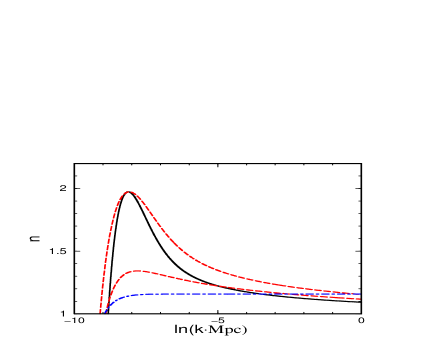
The numerical results for the spectrum of density perturbations did contain a surprise, shown in Fig. 2. While this potential achieved large $n$, slightly smaller than 2, over a few e-folds $n$ falls to a smaller value. Indeed, even restricting the spectrum to astrophysically interesting scales, $1\,$Mpc to $10^{4}\,$Mpc, the spectrum is not a good power law, $|dn/d\ln k|\sim 0.3$, and is reminiscent of the “designer spectra” with special features constructed in Ref. [26]. The reason is simple: in achieving $x^{\prime}\sim 1$ an even larger value of $x^{\prime\prime}$ was attained.

C Example 2

Is there anything special about the hyperbolic sine? Not really – for example, a potential of the form “$\phi+\phi^{3}$” also works. Consider the potential

$$V=V_{0}+M^{4}\left[\left(\frac{\phi-\phi_{1}}{f}\right)+\left(\frac{\phi-\phi_{1}}{f}\right)^{3}+e^{-\textstyle{\frac{\phi}{g}}}\right].$$ (57)

Again, we assume that $V_{0}$ dominates during inflation, that $\phi_{i}=\phi_{60}$ and that $\exp(-\phi/g)$ can be ignored in the inflationary region. To evaluate $N$, we further assume that $|(\phi_{60}-\phi_{1})/f|\gtrsim 1$ and $|(\phi_{f}-\phi_{1})/f|\gtrsim 1$. All of these assumptions are justified by the choice of parameters below.

The analysis of the inflationary constraints is similar. We conclude that large $n$ (here $n=2$) is possible, with the following parameters:

$$V_{0}=1.09\cdot 10^{-12}\,m_{\scriptscriptstyle{PL}}^{4}$$

$$M^{4}=1.46\cdot 10^{-16}\,m_{\scriptscriptstyle{PL}}^{4}$$

$$f=g=1.33\cdot 10^{-2}\,m_{\scriptscriptstyle{PL}}$$

$$\displaystyle{\frac{\phi_{1}}{f}}=13.54$$

$$\displaystyle{\frac{\phi_{f}}{f}}=-1.82$$

$$\displaystyle{\frac{\phi_{60}}{f}}=16.34.$$

This potential is shown in the bottom panel of Fig. 1. Numerical integration of the equation of motion shows that our “60 e-folds” is actually $N_{\rm slowroll}=55.0$ and $N_{\rm exact}=56.0$. Further, just as with the hyperbolic sine potential, $n\sim 2$ is achieved, but the spectrum of perturbations is not a good power law. Both potentials achieve a large change in steepness by having inflation occur near an approximate inflection point; however, the derivative of the change in steepness is also large, and $n$ varies significantly. The change in $n$ can be mitigated at the expense of a smaller value of $n$; see Fig. 2.

IV Conclusions

The deviation of inflationary density perturbations from exact scale invariance ($n=1$) is controlled by the steepness of the potential and the change in steepness, cf. Eq. (8). The steepness of the potential also controls the relationship between the amount of inflation and change in the field driving inflation, $N\sim 8\pi(\Delta\phi/m_{\scriptscriptstyle{PL}})/x$. A very “red spectrum” can be achieved at the expense of a steep potential and prolonged inflation ($t_{f}/t_{i}\gg 1$ and $\Delta\phi\gg m_{\scriptscriptstyle{PL}}$); the simplest example is power-law inflation. A very “blue spectrum” can be achieved at the expense of a large change in steepness near an inflection point in the potential and a poor power law. In both cases there appears to be a degree of unnaturalness.

The robustness of the inflationary prediction of that density perturbations are approximately scale-invariant is expressed by Eq. (43),

$$(n-1)\simeq{2\over N}\ln(x_{i}/x_{f})-{8\pi\over N^{2}}\left({\Delta\phi\over m_{\scriptscriptstyle{PL}}}\right)^{2}.$$

Unless the change in steepness of the potential is large, $|\ln(x_{i}/x_{f})|\gg 1$, or the duration of inflation is very long, $\Delta\phi\gg m_{\scriptscriptstyle{PL}}$, the deviation from scale invariance must be small, $|n-1|\mathrel{\mathchoice{\lower 3.6pt\vbox{\halign{$\mathsurround=0pt\displaystyle\hfil#\hfil$\cr<\crcr\sim\crcr}}}{\lower 3.6pt\vbox{\halign{$\mathsurround=0pt\textstyle\hfil#\hfil$\cr<\crcr\sim\crcr}}}{\lower 3.6pt\vbox{\halign{$\mathsurround=0pt\scriptstyle\hfil#\hfil$\cr<\crcr\sim\crcr}}}{\lower 3.6pt\vbox{\halign{$\mathsurround=0pt\scriptscriptstyle\hfil#\hfil$\cr<\crcr\sim\crcr}}}}{\cal O}(2/N)\sim 0.1$. Even for an extreme range in $n$, say from $n=0.5$ to $n\sim 1.5$, the variation of $\delta_{H}$ over astrophysically interesting scales, $\sim$1 Mpc to $\sim 10^{4}\,$Mpc, is not especially large – a factor of $10$ or so – but is easily measurable.

Inflation also predicts a nearly scale-invariant spectrum of gravitational waves (tensor perturbations). The deviation from scale invariance is controlled solely by the first term in $(n-1)$ [10, 8], $n_{T}=-x_{60}^{2}/8\pi$. Thus, only a red spectrum is possible, with the same remarks applying as for density (scalar) perturbations with $n\ll 1$. In addition, the relative amplitude of the scalar and tensor perturbations is related to the deviation of the tensor perturbations from scale invariance, $T/S\simeq-7n_{T}$ ($S$ and $T$ are respectively the scalar and tensor contributions to the variance of the quadrupole anisotropy of the CBR). Detection of the gravity-wave perturbations is an important, but very challenging, test of inflation; if, in addition, the spectral index of the tensor perturbations can be measured, it provides a consistency test of inflation [25].

Finally, measurements of the anisotropy of the CBR and of the power spectrum of inhomogeneity today which will be made over the next decade will probe the nature of the primeval density perturbations and determine $n$ precisely ($\sigma_{n}\sim 0.01$) [15]. By so doing they will provide a key test of inflation and provide insight into the underlying dynamics. On the basis of our work here, as well as previous studies (see e.g., Ref. [11]), one would expect $(n-1)\sim{\cal O}(0.1)$ or less, but not precisely zero. The determination that $|n-1|\mathrel{\mathchoice{\lower 3.6pt\vbox{\halign{$\mathsurround=0pt\displaystyle\hfil#\hfil$\cr>\crcr\sim\crcr}}}{\lower 3.6pt\vbox{\halign{$\mathsurround=0pt\textstyle\hfil#\hfil$\cr>\crcr\sim\crcr}}}{\lower 3.6pt\vbox{\halign{$\mathsurround=0pt\scriptstyle\hfil#\hfil$\cr>\crcr\sim\crcr}}}{\lower 3.6pt\vbox{\halign{$\mathsurround=0pt\scriptscriptstyle\hfil#\hfil$\cr>\crcr\sim\crcr}}}}{\cal O}(0.2)$, or for that matter $n=1$, would point to a handful of less generic potentials. The deviation of $n$ from unity is a key test of inflation and provides valuable information about the underlying potential [9].

REFERENCES

- [1] A.H. Guth and S.-Y. Pi, Phys. Rev. Lett. 49, 1110 (1982); S.W. Hawking, Phys. Lett. B 115, 295 (1982); A.A. Starobinskii, ibid 117, 175 (1982); J.M. Bardeen, P.J. Steinhardt, and M.S. Turner, Phys. Rev. D 28, 697 (1983).
- [2] M.S. Turner, in Generation of Cosmological Large-scale Structure, edited by D.N. Schramm (Kluwer, Dordrecht, 1998) (astro-ph/9704062).
- [3] E.R. Harrison, Phys. Rev. D 1, 2726 (1970).
- [4] Ya. B. Zeldovich, Mon. Not. R. astron. Soc. 160, 1P (1972).
- [5] J.M. Bardeen, P.J. Steinhardt, and M.S. Turner, Phys. Rev. D 28, 697 (1983).
- [6] P.J. Steinhardt and M.S. Turner, Phys. Rev. D 29, 2162 (1984).
- [7] R. Davis et al, Phys. Rev. Lett. 69, 1856 (1992).
- [8] A. Liddle and D. Lyth, Phys. Lett. B 291, 391 (1992).
- [9] M.S. Turner, Phys. Rev. D. 48, 5539 (1993); J. Lidsey et al, Rev. Mod. Phys. 69, 373 (1997).
- [10] M.S. Turner, Phys. Rev. D 48, 3502 (1993).
- [11] D. Lyth and A. Riotto, Phys. Rept. 314, 1 (1999).
- [12] M. White et al, Mon. Not. Roy. astron. Soc. 283, 107 (1996).
- [13] M. Tegmark, Astrophys. J. 514, L69 (1999).
- [14] J.R. Bond and A. Jaffe, astro-ph/9809043.
- [15] D.J. Eisenstein, W. Hu and M. Tegmark, Ap. J. 518, 2 (1999).
- [16] E.W. Kolb and M.S. Turner, The Early Universe (Addison-Wesley, Redwood City, CA, 1990), Ch. 8.
- [17] A. Kosowsky and M.S. Turner, Phys. Rev. D 52, R1739 (1995).
- [18] A.R. Liddle and M.S. Turner, Phys. Rev. D 50, 758 (1994).
- [19] L Abbott and M. Wise, Nucl. Phys. B 244, 541 (1984).
- [20] F. Lucchin and S. Mattarese, Phys. Rev. D 32, 1316 (1985).
- [21] K. Freese, J.A. Frieman, and A. Olinto, Phys. Rev. Lett. 65, 3233 (1990).
- [22] Y. Hu, M.S. Turner and E.J. Weinberg, Phys. Rev. D 49, 3830 (1994).
- [23] D. Lyth and E. Stewart, Phys. Lett. B 274, 168 (1992).
- [24] A. Linde, Phys. Rev. D 49, 748 (1991).
- [25] M.S. Turner, Phys. Rev. D 55, R435 (1997).
- [26] D. Salopek, J.R. Bond, and J.M. Bardeen, Phys. Rev. D 40, 1753 (1989).