An ASCA Study of the Heavy Element Distribution in Clusters of Galaxies

Abstract

We perform a spatially resolved X-ray spectroscopic study of a set of 11 relaxed clusters of galaxies observed by the ROSAT/PSPC and ASCA/SIS. Using a method which corrects for the energy dependent effects of the ASCA PSF based on ROSAT images, we constrain the spatial distribution of Ne, Si, S and Fe in each cluster. Theoretical prescriptions for the chemical yields of Type Ia and II supernovae, then allow determination of the Fe enrichment from both types of supernovae as a function of radius within each cluster. Using optical measurements from the literature, we also determine the iron mass-to-light ratio (IMLR) separately for Fe synthesized in both types of supernovae. For clusters with the best photon statistics, we find that the total Fe abundance decreases significantly with radius, while the Si abundance is either flat or decreases less rapidly, resulting in an increasing Si/Fe ratio with radius. This result indicates a greater predominance of Type II SNe enrichment at large radii in clusters. On average, the IMLR synthesized within Type II SNe increases with radius within clusters, while the IMLR synthesized within Type Ia SNe decreases. At a fixed radius of 0.4 $R_{virial}$ there is also a factor of 5 increase in the IMLR synthesized by Type II SNe between groups and clusters. This suggests that groups expelled as much as 90% of the Fe synthesized within type II SNe at early times. All of these results are consistent with a scenario in which the gas was initially heated and enriched by Type II SNe driven galactic winds. Due to the high entropy of the preheated gas, SN II products are only weakly captured in groups. Gravitationally bound gas was then enriched with elements synthesized by Type Ia supernovae as gas-rich galaxies accreted onto clusters and were stripped during passage through the cluster core via density-dependent mechanisms (e.g. ram pressure ablation, galaxy harassment etc.). We suggest that the high Si/Fe ratios in the outskirts of rich clusters may arise from enrichment by Type II SNe released to ICM via galactic star burst driven winds. Low S/Fe ratios observed in clusters suggest metal-poor galaxies as a major source of SN II products.

1. Introduction

Understanding the formation and evolution of large structures like groups and clusters of galaxies is one of the main goals of contemporary astrophysics. The presence of hot X-ray emitting gas in clusters is an invaluable diagnostic of the dynamic, thermodynamic, and chemical state of clusters. The discovery of Fe-K line emission in cluster spectra by Mitchell et al. (1976) and Serlemitsos et al. (1977) was the first indication that some of the hot intracluster gas originated within galaxies. Heavy elements can be supplied to the cluster gas through galactic winds (De Young 1978; David, Forman, and Jones 1991; White 1991; Metzler & Evrard 1994) and ram pressure stripping (Gunn and Gott 1971). Estimates of the iron abundance in clusters from HEAO-1, Exosat, Ginga, and ROSAT observations show that most rich clusters have iron abundances that range between 25%-50% of the solar value. Arnaud et al. (1992) showed that there is a strong correlation between the Fe mass in rich clusters and the luminous mass in E and S0 galaxies. Such a correlation suggests that, at least in rich clusters, the iron may predominantly originate from early type galaxies. Even though the Fe abundances in clusters are typically sub-solar, there is a considerable amount of Fe in the intracluster medium since the hot gas comprises approximately 5 times the luminous mass in galaxies (David et al. 1990, Arnaud et al. 1992). As noted by Renzini (1997), the Fe mass-to-light ratio (IMLR) for the hot gas in clusters is typically $\sim$0.02 $M_{\odot}$/$L_{\odot}$  and is several times larger than that locked up in stars. Thus, not only does the hot gas contain most of the baryons in clusters, it also contains most of the heavy elements.

Table 1X-ray and optical quantities of the sample

Name	DL	1′	$L_{B}$	$R_{mes}$	$L_{B,N_{0.5}}$	$L_{B_{cD}}$	$R_{c}$	$\beta_{out}$	$r_{out}$	$T_{e}$	$\delta T_{e}$	$R_{virial}$
	Mpc	kpc	$10^{11}$$L_{\odot}$	Mpc	$10^{11}$$L_{\odot}$	$10^{11}$$L_{\odot}$	Mpc		kpc	keV	keV	Mpc
A496	199	53			10.9†	1.35	0.39	0.70	250	4.7	0.2	2.67
A780	346	90			9.4†		0.24	0.66	120	4.3	0.4	2.56
A1060	69	19			5.42	1.22	0.24	0.70	161	3.1	0.1	2.18
A1651	520	128			15.9†		0.24	0.70	260	6.1	0.4	3.05
A2029	470	118			22.53	2.53	0.22	0.68	280	9.1	1.1	3.72
A2199	181	50			10.91	2.19	0.24	0.64	140	4.8	0.2	2.70
A2597	520	129			9.7†	0.40	0.24	0.68	180	4.4	0.4	2.59
A2670	465	117	26.18	3.10	9.1†	0.55	0.24	0.55	113	4.2	0.6	2.53
A3112	461	116			12.9†	2.59	0.24	0.63	120	5.3	0.8	2.84
A4059	291	77			9.7†	1.04	0.24	0.67	220	4.4	0.3	2.59
MKW4	121	33	14.80	10.25		1.78	0.17	0.64	180	1.7	0.1	1.60
AWM7	104	29	18.80	9.21	6.89	1.90	0.22	0.53	102	3.5	0.2	2.31
HCG51	156	43	2.80	1.19		—	0.06	0.30	78	1.3	0.1	1.43
HCG62	82	23	0.95	1.09		—	0.03	0.30	52	1.1	0.1	1.30
N5044	54	15	2.30	0.5		0.68	0.18	0.51	11	1.2	0.1	1.37
Virgo	17	5	9.60	3.0	4.73	1.05	0.24	0.45	11	2.7	0.2	2.03

^†    Estimated value using Eq.1

To determine the exact origin of the heavy elements in clusters requires information on the abundance of several heavy elements which is now possible with ASCA. Galactic winds primarily occur at early times and enrich the intergalactic medium with type II SN ejecta which is abundant in $\alpha$-process elements. Ram pressure stripping of galaxies occurs over a longer period as clusters continuously accrete field galaxies and enrich the intergalactic medium with type Ia SN ejecta which is abundant in Fe. Loewenstein & Mushotzky (1996) showed that the abundance ratios of $\alpha$-process elements relative to Fe outside the central regions of four rich clusters was similar to that of type II SN ejecta. Fukazawa et al. (1998) have shown that globally averaged Fe abundances outside cluster cores are nearly independent of gas temperature, while Si abundances increase significantly with gas temperature. This suggests that there is an increasing predominance of type II SN in the enrichment process of richer clusters. In general, the heavy elements that originate from type II SN are a direct measure of the stellar initial mass function (IMF) and the gas retention ability of clusters.

In Finoguenov & Ponman (1999), we demonstrated that both SN Ia and SN II make a significant contribution to the enrichment of the intergalactic medium by comparing the metal content of groups with that of a cluster of galaxies. We found that SN II products are widely distributed within the IGM, which probably indicates that the ejecta were released at early times in the formation of clusters via energetic galactic winds. The observed iron mass-to-light ratios indicate that rich clusters retained the SN II products more efficiently than groups at all radii from 0.05 to at least 0.4 of $R_{virial}$. In contrast, the distribution of Fe attributed to SN Ia is more centrally peaked, with a core radius comparable to the optical radius of the system. This indicates that the primary gas enrichment mechanism is strongly density-dependent, such as gas ablation, ram pressure stripping, or galaxy-galaxy interactions.

In this Paper, we present an extensive study of the distribution of heavy elements in groups and clusters and discuss the implications regarding the chemical enrichment process of the intracluster medium. The elemental abundances are determined using 3-dimensional modeling of ASCA/SIS data. This procedure takes advantage of the higher spatial resolution ROSAT observations, which are used to model the effect of the broader, energy dependent PSF of the ASCA XRT on the distribution of detected events in the ASCA focal plane. We present new spectroscopic analysis for MKW4, A496, A780, A1060, A1651, A2029, A2199, A2597, A2670, A3112, and A4059. This sample, contains almost all of the 4 keV clusters observed by ASCA, for which we can determine the abundance of several heavy elements. Our sample also contains MKW4 and A1060, which are slightly cooler, and A2029 and A1651 which are slightly hotter. To complete our sample, we include previously published results on M87 (Finoguenov & Jones 2000); AWM7 (Finoguenov & Ponman 1999); and the groups NGC5044, HCG51, and HCG62 (Finoguenov & Ponman 1999), which sample the low-temperature end of the cluster distribution.

This paper is organized as follows: in section 2 we describe our analysis technique; we then present the radial abundance profiles of Fe, Si, Ne and S in section 3, and analyze the spatial distribution of abundance ratios in our cluster sample in section 4. In section 5 we discuss the relative importance in the overall enrichment process of different types of supernovae. Our main results are summarized in section 6 along with a discussion about their implications for cluster evolution. We assume $H_{\rm o}=50$ km s^-1 Mpc^-1 and $q_{\rm o}$$=0.5$ throughout the paper.

2. Data Reduction

A detailed description of the ASCA observatory as well as the SIS detectors can be found in Tanaka, Inoue & Holt (1994) and Burke et al. (1991). All observations are screened using FTOOLS version 4.1 with standard screening criteria. The effect of the broad ASCA PSF is treated as described in Finoguenov et al. (1999), including the geometrical projection of the three-dimensional distribution of X-ray emitting gas. Our minimization routines are based on the $\chi^{2}$ criterion. No energy binning is done, but a special error calculation is introduced as in Churazov et al. (1996), to properly account for small number statistics.

Model fits to ROSAT (Truemper 1983) surface brightness profiles are used as input to the ASCA data modeling. The ROSAT results are used to define the shape of the X-ray profile within each spatial bin used for the ASCA analysis. Our analysis therefore assumes that the ASCA and ROSAT surface brightness profiles have the same shape. This shape affects the amount of coupling (due to projection and PSF blurring) between the ASCA spectra, which is allowed for in the simultaneous fitting process. However, the normalization of the flux in each ASCA bin is not determined by the ROSAT profile, but is free to fit to the ASCA data. Hence any difference in emission between the soft (ROSAT) and harder bands, due to possible temperature gradients or the presence of multiphase gas, has only a second order effect on our analysis, via changes in profile shape with energy. Moreover, the effects of any such energy variations must reduce as smaller spatial bins are used for the analysis, since as the radial bins shrink towards zero width, these factors are known from the ASCA PSF calibration alone, and does not depend on the ROSAT data at all. In checking the effects of systematics, we have varied the spatial binning to quantify the effect on our modeling of possible differences between profiles in the ROSAT and ASCA bands, near the cluster center.

For regions with complex structure (e.g.  the central part of A2670 which has a bimodal structure), we used the actual PSPC image (rather than just its radial profile) as a basis for the ASCA modeling. For all ROSAT imaging analysis, we use the software described in Snowden et al. (1994) and references therein. The details of our minimization procedure for ASCA spectral analysis are described in Finoguenov and Ponman (1999).

We adapted the XSPEC analysis package to perform the actual fitting and error estimation. Fluctuations in spectral properties are constrained using a regularization technique (Press et al. 1992; Finoguenov and Ponman 1999), but the solution returned is always required to lie within 90% confidence of the best fit. Since regularization effectively couples the values returned for the spectral properties at neighboring points, we display the error regions as continuous bands in the Figures below.

Table 2ASCA SIS observational log.

		SIS0	SIS1
Name	seq. #	exp.	exp.
		ksec	ksec
A496	80003000	31	23
	86069000	22	22
	86069010	6	24
A780	80015000	14	12
A1060	80004000	30	22
A1651	82036000	32	30
A2029	81023000	29	28
	83040010	6	—
	83040020	3	—
A2199	80023000	21	16
	86068000	19	19
	86068010	22	22
A2597	83062000	36	34
A2670	82049000	17	13
A3112	81003000	25	16
A4059	82030000	28	27
MKW4	52027000	47	50
	82012000	12	6
	82013000	13	6
	82014000	11	4

The MEKAL plasma code (Mewe et al. 1985, Mewe and Kaastra 1995, Liedahl et al. 1995) has been used for all of our spectral analysis. Abundances are given relative to the solar values in Anders & Grevesse (1989). The abundances of He and C are fixed to solar values. The remaining elements are combined into five groups for fitting: Ne; Mg; Si; S and Ar; and Ca, Fe, and Ni. We restrict our analysis to the energy range 0.8–7.0 keV to avoid the large systematic uncertainties at low energies, which also prevent us from determining the O abundance. We do not report the Mg abundance due to the proximity of the Mg K lines to the poorly understood 4-2 transition lines of iron, which are strongest at temperatures of 2 to 4 keV (see Fabian et al. 1994 and Mushotzky et al. 1996).

The presence of a central cooling flow in some clusters further complicates the spectral analysis. In such cases, we have applied three different models for the cooling flow emission, within the central one or two spatial bins: (a) a standard XSPEC cooling flow model (mkcflow) plus a thermal component (MEKAL) of the same temperature as the maximum temperature in the cooling flow model, (b) a realization of the code of Wise & Sarazin (1993) for cooling flow plus an isothermal component similar to that in (a), and (c) a two-temperature model (Buote 1999). In each model, element abundances were assumed to be the same in both components, except in the case of Virgo, where they were fitted separately and shown to be the same (Finoguenov & Jones 2000). The two-temperature model was found to most strongly reduce the luminosity of the primary temperature component. Using this model within the cooling region, the gas distribution from the hot component was found to be a good extrapolation of a beta-model fit to ROSAT data from the data outside the cooling region.

The addition of a cooling flow component was found to have little effect on element abundance determination in the hotter systems. However, for systems whose temperature and abundance determination relies on the Fe L-shell emission, introduction of the two-temperature component strongly affects the stability of the solution, due to the inadequate energy resolution of our CCD measurements. Among the systems, studied in this paper, HCG51, HCG62, NGC5044 and MKW4 fall into this category. We discuss the implication of this effect for the credibility of the corresponding abundance determinations in the Appendix. Following Finoguenov & Jones (2000), we add 10% systematic error below 1.5 keV in spectral analysis, whenever we determine the Fe abundance from the L-shell line complex.

No simple correlation was found between our cooling flow mass drop rate estimations and the strength of abundance gradients. However, the suggestion of Allen and Fabian (1998) that non-cooling flow clusters have lower central iron abundance due to recent mergers, explains the abundance profile of A2670. A2670 was included in our analysis first and in adding other clusters to our sample we specially avoided indications of merger, so it is not surprising that perhaps ’too many’ our clusters show abundance gradients.

Following a suggestion of the referee, we explore the effects of ASCA PSF systematics as well as the sensitivity of our results to changes in the modeling of the ROSAT surface brightness distribution. The effects of PSF variations were explored using simulations, as in Markevitch et al. (1998). The calibration uncertainty in the ASCA PSF estimation was adopted as 10% at the 68% confidence level. In our spectral analysis, we account for the effects of the PSF using a scattering matrix (Finoguenov et al. 1999). In simulating the effect of systematic PSF errors, we create a number of different scattering matrices. The resulting systematic uncertainty in the interesting parameters was calculated as the RMS of their best-fit values obtained using different scattering matrices.

Variations in the surface brightness representation were investigated by using the results of Mohr et al. (1999), which were derived using a surface brightness fitting technique different from our own. Uncertainties in the PSF and ROSAT profiles were found to have significant effects on normalization and somewhat on the temperature, but little impact on the element abundance determinations. We have included the effects of systematics in the parameter’s uncertainties, presented in this paper. We have also checked the effect of the elliptical geometry of some clusters by taking the actual ROSAT image (as an alternative to its radial profile) as the basis for modeling the flux distribution in A4059, which is the most elliptical of our clusters. The results of this, of variations in the treatment of the central cooling flow, and of uncertainties in the ASCA PSF, are all shown for A4059 in Fig.1. It can be seen that the abundance distribution is quite robust to such differences in the analysis, with systematic variations being confined within the 90% statistical error region.

As discussed above, any errors in our analysis resulting from differences between X-ray profiles in the ROSAT and ASCA energy bands should reduce as smaller spatial bins are used for the analysis. Within the limits set by the increasing effects of ASCA PSF systematics, when going to smaller spatial bins (Markevitch private communication) we have checked whether our assumption of the spectral-spatial separability of the emission (Finoguenov et al. 1999) affects our final results, by increasing the number of spatial bins. Since no significant changes in element distributions were obtained, we conclude that this assumption is reasonable.

Table 1 contains the optical and X-ray properties of our sample. Column (1) identifies the system, (2) adopted luminosity distance, (3) corresponding scale length, (4–5) total blue light and radius for this measurement, (6) estimated blue luminosity within 0.5 Mpc based on the Bahcall (1981) central galaxy density within 0.5 Mpc, (7) luminosity of dominant central galaxy (referred to throughout the present paper as a ‘cD’), and (8) core radius of the galaxy distribution. Cols. (9–10) give the results of the cluster surface brightness fitting with a $\beta$ model, taken from Vikhlinin, Forman, Jones (1999), where regions contaminated by the cooling flow were excluded from the analysis, supplemented by data from Finoguenov and Ponman (1999), Finoguenov and Jones (2000), (11) gives the best fit cluster emission-weighted temperature, (12) the corresponding 90% error, (13) the virial radius of the system ($r_{180}=1.23T_{keV}^{0.5}h_{50}^{-1}$ Mpc; Evrard et al. 1996).

The observation log for the cluster sample is given in Table 2. The SIS exposure times are based on applied standard screening. For the new data, analyzed here, distances were taken from compilation of Vikhlinin et al. (1999). Optical luminosities are obtained from the compilation in Arnaud et al. (1992), converting from V to B using $B=V+0.94$. Optical measurements for MKW4 and AWM7 are taken from Beers et al. (1984). For A780 and A1651 no data on luminosity of the cD galaxy was located. Core radii are obtained from Girardi et al. (1995). For clusters without a measured core radius, we use the mean value of 0.24 Mpc from Girardi et al. (1995). For MKW4 we derived the core radius from data in Dell’Antonio, Geller & Fabricant (1995). For A496, a measurement of the core radius was taken from Whitmore et al. (1993). Cluster data in cols. (11-12) is taken from GIS temperature estimates by Markevitch et al. (1998). The emission weighted temperatures in cols. (11-12) for the low-temperature systems are derived from our SIS spectral analysis and are corrected for the presence of cooling flows.

The new temperature data on MKW4 and A1060, derived in this paper are presented in Tab.2. We see evidence for a declining temperature in both MKW4 and A1060. The later system is often cited as an example of an isothermal cluster (Tamura et al. 1996), however their recent reanalysis of the data agrees with our findings (Tamura et al. 2000).

New ASCA SIS temperature measurements^†‡

Annulus (′)	$kT_{e}$	Annulus (′)	$kT_{e}$
MKW4		A1060
0.0—1.5	1.770 (1.50:1.80)	0.0—0.8	4.36 (3.0:6.0)
1.5—2.9	1.781 (1.72:1.85)	0.8—1.5	4.19 (3.3:5.3)
2.9—5.5	1.779 (1.72:1.85)	1.5—2.4	3.83 (3.4:4.3)
5.5—10.5	1.650 (1.59:1.70)	2.4—3.9	3.27 (2.9:3.6)
10.5—20.	1.478 (1.39:1.58)	3.9—6.2	3.05 (2.8:3.3)
		6.2—10.	3.34 (3.0:3.6)
		10.—16.	2.69 (2.5:2.8)

1. Errors are given at 68% confidence level for one parameter of interest. MEKAL plasma code is used for spectral fitting.

2. For the rest of the clusters analyzed in this paper, the combined GIS+SIS+PSPC temperature measurements of Markevitch et al. (1998) supersede our data

For clusters without published optical luminosities, the luminosities are derived from the correlation between the X-ray temperature and the Bahcall number density, $N_{0.5}$ (Edge & Stewart 1991), the latter is directly related to optical luminosity within 0.5 Mpc (cf Edge & Stewart 1991). Since the correlation found in Edge & Stewart (1991) has such a large scatter, we recalibrated it using ASCA measured temperatures (Markevitch et al. 1998 and this paper) and find a best fit relation given by:

Cluster gas temperature vs galaxy number density (the Bahcall number) within 0.5 Mpc. The solid line indicates our best-fit relation, and the dashed line indicates the best-fit relation obtained by Edge and Stewart (1991). Error bars are shown at the 90% confidence level. In order of increasing Bahcall number, the points correspond to Virgo, A1060, AWM7, A2199, A1795, A2141, A2029 and A401.

$$N_{0.5}=3.46\pm 0.6\;\times\;T^{1.058\pm 0.06}$$ (1)

where $T$ is in units of keV. The errors are given at the 90% confidence level. As can be seen in the figure, the scatter about this line is remarkably small, corresponding to 20% in $N_{0.5}$. While our best-fit relation is within the uncertainties of Edge and Stewart (1991), their best-fit prediction deviates somewhat from the data on the cool clusters Virgo, AWM7, and A1060 (see Fig.2). However, since in practice we only use Eq.1 to estimate the cluster blue luminosities for clusters in the range 4–6 keV, no significant difference would occur if their relation were used.

3. Radial Distribution of Heavy Elements

The abundance data, derived in this work, are tabulated in Table 3.

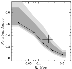
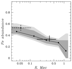
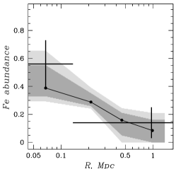
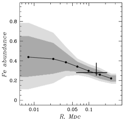
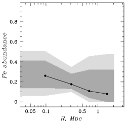
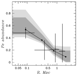
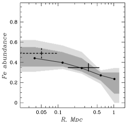
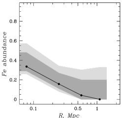
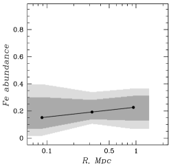
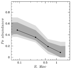
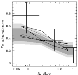
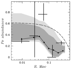
Figure 1.— Derived Fe abundances (in units of 4.68 $10^{-5}$ for iron number abundances relative to H). The solid lines correspond to the best-fit Fe abundances derived from the ASCA data. The filled circles indicate the spatial binning used in the analysis. Dark and light shaded zones around the best fit curves denote the 68 and 90 per cent confidence areas. Crosses on the A2029 panel represent previous ASCA SIS+GIS results from Sarazin et al. (1998). Solid crosses on the A496, A1060 and A2199 panels show the results from Mushotzky et al. (1996). A cross on the MKW4 panel shows the results from Fukazawa et al. (1998) with radii of measurement from Fukazawa (private communication). Crosses on the A780 plot denote the results of modeling of GIS data from Ikebe et al. (1997) and similarly on the A4059 plot from Kikuchi et al. (1999). Dashed crosses on the A496 and A2199 panels show abundance determinations from Dupke & White (1999). On the A4059 panel we illustrate the effect of the inclusion of a different cooling flow model (short-dashed line), ASCA PSF systematics (dotted lines) and usage of the ROSAT image as an input (long-dashed lines for two extreme solutions). On the HCG62 panel we also show the results obtained when the regularization in spectral fitting is turned off (solid crosses). This is discussed in the Appendix. The dashed line indicates the results of an independent analysis of ROSAT PSPC data, as discussed in Finoguenov & Ponman (1999).

MKW4      A496      A780    A1060  

A1651    A2029    A2199    A2597   

A2670    A3112    A4059    HCG62   

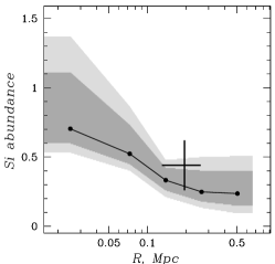
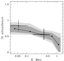
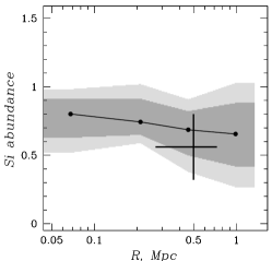
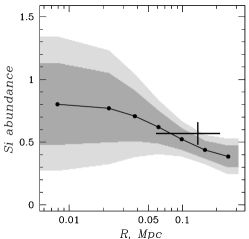
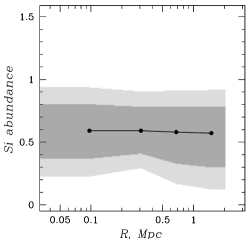
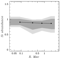
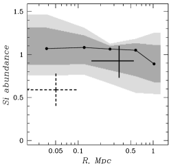
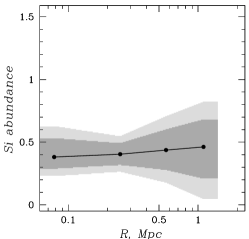
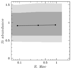
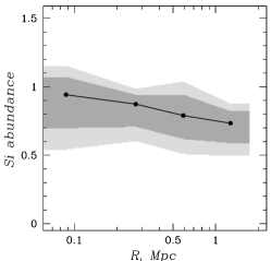
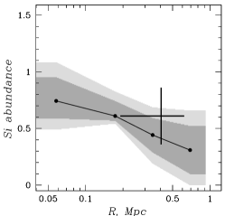
Figure 2.— Derived Si abundances. The solid lines correspond to the best-fit Si abundances derived from the ASCA data. The filled circles indicate the spatial binning used in the analysis. Dark and light shaded zones around the best fit curve denote the 68 and 90 per cent confidence areas, respectively. Solid crosses on the A496, A1060 and A2199 panels represent ASCA values from Mushotzky et al. (1996). Crosses on MKW4, A780 and A4059 panels represent ASCA values from Fukazawa et al. (1998), with radii of measurements from Fukazawa (private communication). Dashed crosses on the A496 and A2199 panels show abundance determinations from Dupke & White (1999).

MKW4      A496      A780    A1060  

A1651    A2029    A2199    A2597   

A2670                        A3112                        A4059   

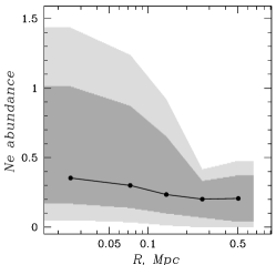
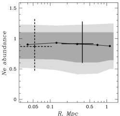
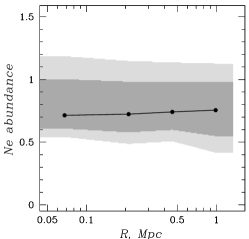
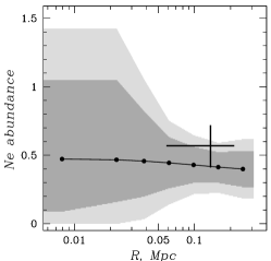
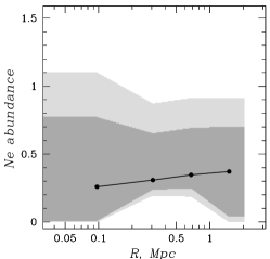
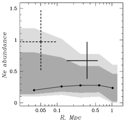
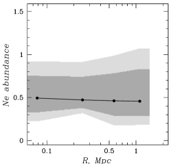
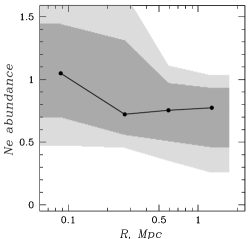
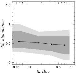
Figure 3.— Derived Ne abundances. Solid line represents the best-fit curve describing ASCA results, with filled circles indicating the spatial binning used. Dark and light shaded zones around the best fit curve denote the 68 and 90 per cent confidence areas, respectively. Solid crosses on the A496, A1060 and A2199 panels represent ASCA values from Mushotzky et al. (1996). Dashed crosses on the A496 and A2199 panels show abundance determinations from Dupke & White (1999).

MKW4                         A496                        A780   

A1060                        A1651                        A2199   

A2597                        A3112                        A4059   

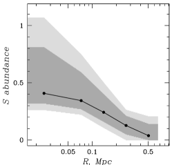
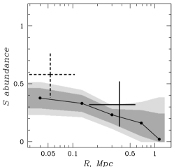
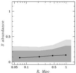
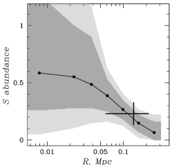
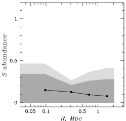
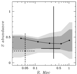
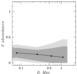
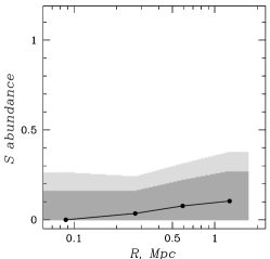
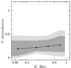
Figure 4.— Derived S abundances. Solid line represents the best-fit curve describing ASCA results, with filled circles indicating the spatial binning used. Dark and light shaded zones around the best fit curve denote the 68 and 90 per cent confidence areas, respectively. Solid crosses on the A496, A1060 and A2199 panels represent ASCA values from Mushotzky et al. (1996). S is coupled with Ar in our fitting, so our limits are sometimes more strict in comparison to the values of Mushotzky et al. (1996). Dashed crosses on the A496 and A2199 panels show abundance determinations from Dupke & White (1999).

MKW4                         A496                        A780   

A1060                        A1651                        A2199   

A2597                        A3112                        A4059   

Table 3ASCA SIS heavy element abundance measurements^†

Annulus (′)	$Ne/Ne_{\odot}$	$Si/Si_{\odot}$	$S/S_{\odot}$	$Fe/Fe_{\odot}$
MKW4
0.0—1.5	0.35 (0.17:1.01)	0.70 (0.60:1.11)	0.41 (0.32:0.81)	0.62 (0.58:0.89)
1.5—2.9	0.30 (0.14:0.87)	0.52 (0.45:0.73)	0.34 (0.27:0.59)	0.45 (0.41:0.62)
2.9—5.5	0.23 (0.10:0.65)	0.33 (0.26:0.42)	0.24 (0.16:0.40)	0.26 (0.22:0.44)
5.5—10.5	0.20 (0.07:0.33)	0.25 (0.18:0.40)	0.13 (0.05:0.21)	0.13 (0.10:0.24)
10.5—20.0	0.21 (0.04:0.37)	0.24 (0.15:0.40)	0.04 (0.00:0.14)	0.06 (0.03:0.11)
A496
0.0—1.5	0.90 (0.67:1.10)	0.74 (0.63:0.86)	0.38 (0.29:0.46)	0.47 (0.43:0.55)
1.5—3.4	0.93 (0.66:1.10)	0.65 (0.59:0.80)	0.33 (0.26:0.40)	0.39 (0.34:0.48)
3.4—8.0	0.91 (0.61:1.10)	0.56 (0.49:0.65)	0.23 (0.16:0.28)	0.31 (0.26:0.36)
8.0—18.0	0.90 (0.61:1.10)	0.50 (0.37:0.60)	0.16 (0.05:0.27)	0.27 (0.22:0.31)
18.0—25.0	0.88 (0.65:1.10)	0.24 (0.02:0.46)	0.02 (0.00:0.24)	0.13 (0.00:0.31)
A780
0.0—1.5	0.71 (0.61:1.00)	0.80 (0.63:0.91)	0.08 (0.00:0.22)	0.39 (0.33:0.55)
1.5—3.2	0.72 (0.58:0.98)	0.74 (0.65:0.91)	0.10 (0.00:0.22)	0.29 (0.26:0.35)
3.2—7.0	0.74 (0.60:0.98)	0.69 (0.50:0.82)	0.13 (0.00:0.25)	0.16 (0.05:0.21)
7.0—15.0	0.76 (0.55:0.98)	0.66 (0.42:0.88)	0.14 (0.00:0.32)	0.08 (0.00:0.16)
A1060
0.0—0.8	0.47 (0.09:1.05)	0.80 (0.48:1.13)	0.59 (0.26:1.27)	0.44 (0.24:0.65)
0.8—1.5	0.47 (0.16:1.05)	0.77 (0.50:1.05)	0.55 (0.28:1.00)	0.42 (0.27:0.58)
1.5—2.4	0.46 (0.20:0.82)	0.71 (0.51:0.91)	0.49 (0.28:0.90)	0.39 (0.30:0.48)
2.4—3.9	0.44 (0.26:0.63)	0.62 (0.49:0.75)	0.39 (0.25:0.53)	0.34 (0.29:0.39)
3.9—6.2	0.43 (0.30:0.56)	0.52 (0.44:0.61)	0.27 (0.18:0.35)	0.30 (0.26:0.34)
6.2—10.0	0.41 (0.30:0.52)	0.44 (0.37:0.51)	0.15 (0.07:0.22)	0.26 (0.22:0.30)
10.0—16.0	0.40 (0.27:0.53)	0.39 (0.30:0.47)	0.07 (0.00:0.16)	0.22 (0.19:0.25)
A1651
0.0—1.5	0.26 (0.01:0.77)	0.59 (0.37:0.80)	0.15 (0.00:0.34)	0.26 (0.14:0.41)
1.5—3.3	0.31 (0.24:0.65)	0.59 (0.41:0.78)	0.13 (0.00:0.21)	0.18 (0.13:0.28)
3.3—7.3	0.35 (0.25:0.69)	0.58 (0.33:0.78)	0.10 (0.00:0.26)	0.11 (0.04:0.32)
7.3—16.0	0.37 (0.04:0.70)	0.57 (0.30:0.78)	0.08 (0.00:0.28)	0.08 (0.00:0.32)
A2029
0.0—1.5		0.91 (0.81:1.01)		0.53 (0.46:0.73)
1.5—3.8		0.88 (0.66:0.95)		0.36 (0.33:0.46)
3.8—9.5		0.87 (0.72:0.95)		0.19 (0.14:0.24)
9.5—24.0		0.86 (0.68:1.01)		0.09 (0.01:0.19)
A2199
0.0—1.5	0.20 (0.14:0.80)	1.07 (0.88:1.31)	0.48 (0.25:0.52)	0.44 (0.36:0.55)
1.5—3.3	0.26 (0.18:0.72)	1.08 (0.89:1.22)	0.41 (0.28:0.46)	0.40 (0.36:0.50)
3.3—7.3	0.28 (0.16:0.58)	1.06 (0.82:1.10)	0.38 (0.27:0.50)	0.34 (0.31:0.44)
7.3—16.0	0.28 (0.17:0.58)	1.05 (0.75:1.13)	0.37 (0.26:0.52)	0.27 (0.22:0.30)
16.0—25.0	0.24 (0.02:0.46)	0.89 (0.68:1.11)	0.44 (0.22:0.65)	0.23 (0.09:0.30)
A2597
0.0—1.2	0.49 (0.33:0.75)	0.38 (0.29:0.53)	0.19 (0.10:0.29)	0.34 (0.29:0.48)
1.2—2.7	0.47 (0.38:0.74)	0.40 (0.32:0.49)	0.17 (0.04:0.25)	0.16 (0.11:0.27)
2.7—6.1	0.46 (0.29:0.78)	0.44 (0.28:0.60)	0.13 (0.00:0.28)	0.04 (0.00:0.20)
6.1—11.0	0.46 (0.29:0.83)	0.46 (0.21:0.68)	0.11 (0.00:0.32)	0.00 (0.00:0.20)
A2670
0.0—1.5		0.91 (0.64:1.27)		0.15 (0.07:0.30)
1.5—4.0		0.93 (0.64:1.30)		0.19 (0.14:0.28)
4.0—12.0		0.94 (0.64:1.30)		0.23 (0.13:0.31)
A3112
0.0—1.5	1.05 (0.70:1.44)	0.94 (0.70:1.07)	0.00 (0.00:0.16)	0.48 (0.41:0.62)
1.5—3.2	0.72 (0.56:1.31)	0.87 (0.71:0.94)	0.04 (0.00:0.16)	0.36 (0.30:0.48)
3.2—7.0	0.75 (0.51:0.97)	0.79 (0.62:0.94)	0.08 (0.00:0.22)	0.19 (0.11:0.27)
7.0—15.0	0.77 (0.46:0.93)	0.73 (0.59:0.82)	0.10 (0.00:0.27)	0.09 (0.00:0.20)
A4059
0.0—1.5	0.55 (0.39:0.83)	0.74 (0.59:0.95)	0.19 (0.04:0.36)	0.44 (0.36:0.60)
1.5—3.0	0.52 (0.34:0.69)	0.61 (0.57:0.74)	0.22 (0.14:0.36)	0.37 (0.32:0.44)
3.0—6.0	0.48 (0.30:0.69)	0.44 (0.29:0.59)	0.24 (0.13:0.38)	0.27 (0.22:0.34)
6.0—12.0	0.46 (0.22:0.69)	0.31 (0.10:0.52)	0.27 (0.12:0.46)	0.21 (0.14:0.31)

1. Definition of the solar abundance units is 12.3, 3.55, 1.62 and 4.68 $\times 10^{-5}$ for the number abundance of Ne, Si, S and Fe relative to H, respectively. Errors are given at 68% confidence level (see text for further details). MEKAL plasma code is used for spectral fitting.

3.1. Iron

Significant Fe abundance gradients are detected in MKW4, A496, A780, A2029, A2199, A2597 and A3112 (see Fig. 1). An Fe abundance gradient was previously reported for A780 by Ikebe et al. (1997) using GIS data. Detection of an Fe abundance gradient in A4059 using the wider field of view of the GIS (Kikuchi et al. 1999) is in agreement with the trend seen in our SIS analysis. Sarazin et al. (1998) reported a marginal Fe abundance gradient in A2029 based on the central ASCA pointing alone. Beyond the cooling flow region in the clusters, we find good agreement between the Fe abundances derived from our three-dimensional modeling technique with those obtained from previous estimates (e.g. Mushotzky et al. 1996 and Fukazawa et al. 1998), as well as the central abundances estimated in Dupke and White (1999).

At a radial distance of 1 Mpc, all clusters have an iron abundance below 0.3 solar. The mean Fe abundance at 1 Mpc is 0.20 solar with an rms of 0.10. Due to the presence of Fe abundance gradients, the Fe abundance in the central spatial bin is sensitive to the physical width of the bin, so nearby systems have higher inferred central abundances. Most of the systems have central Fe abundances in excess of 0.4 solar. The exceptions are A2670 and probably A1651, which do not have observed Fe abundance gradients, which makes them candidates for recent mergers. A2670 may be undergoing a merger based on optical (Bird 1994) and ROSAT PSPC (Hobbs and Willmore 1997) observations.

3.2. Silicon

The Si distribution within the clusters in our sample is, in general, more spatially uniform than the Fe distribution. Even in MKW4, where there is a noticeable Si gradient, the decline in the Si abundance is not as strong as the decline in the Fe abundance. In most clusters, the Si abundance is fairly uniform at 30–50% of the solar value. The only group in our sample, MKW4, has a significantly lower Si abundance than the clusters. This is in agreement with the general trend noted by Fukazawa et al. (1998).

Ponman, Cannon & Navarro (1999) examined the density distribution in a sample of clusters, and concluded that supernova-driven winds were probably only efficient in reducing the content of gas and metals in clusters with virial temperatures below approximately 4 keV. The approximately flat distribution of Si for clusters hotter than about 4 keV suggests that either alpha-elements have been injected uniformly through the cluster by some non-density dependent mechanism, or that the intergalactic gas has been well mixed since the bulk of these elements were injected. The observed scatter of Si abundances in our sample could be an indication of detailed differences in the evolution of individual clusters (we return to this subject below).

3.3. Neon

The results concerning the Ne distribution are similar to that of Si, except that the errors are larger. As with Si, Ne gradients are not seen at a high significance. The Ne abundance in A2670 and A2029 are highly uncertain, and we do not present the results here. The large uncertainties in the best fit Ne abundances smear out the differences among the systems. In a few cases (A496, A780, A2597 and A3112), the best fit Ne abundance at a radial distance of 1 Mpc is constrained to be between $\sim 0.3$ and solar, while for the remainder of the systems it is only constrained to be less than solar.

The derived Ne abundances are affected by the inclusion of a cooling flow model, and also dependent on the model adopted for the cooling flow. This is due to the fact that the Ne lines lie at nearly the same energy as the L-shell Fe blend, so that emission from cooling gas can be confused with Ne emission. In presenting the Ne results, we take the best fit values based on the spectral analysis that includes a mkcflow model, while the errors include the variance observed between different models, including simple single temperature fits.

3.4. Sulfur

By coupling the abundances of S and Ar, we obtain errors smaller than the errors listed in Mushotzky et al. (1996). Even with this coupling, the uncertainties in the S and Ar abundances in A2670 and A2029 are large, and we do not present the results for these two clusters. A central enhancement in sulfur in detected in MKW4 and marginally in A1060 and A496 (see Fig.4). For the remainder of the sample, the spectroscopic results are consistent with a uniform sulfur distribution with values of 50–100% the solar value.

The sulfur abundance at a radius of 1 Mpc is less then 0.5 solar in all the systems in our sample. Definite non-zero values for the S abundance at 1 Mpc are only detected in A2199, and definite non-zero values at all radii within a cluster could only be obtained in five systems (MKW4, A496, A1060, A2199 and A4059).

vs radius. Grey lines represent groups and black lines represent clusters. The statistical uncertainty in the data increases with radius from about 0.05 in the central regions to about 0.2 at 1 Mpc in terms of [Si/Fe] at the 90% confidence level. A2670 has a large uncertainty in [Si/Fe] and is omitted from the plot.

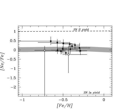
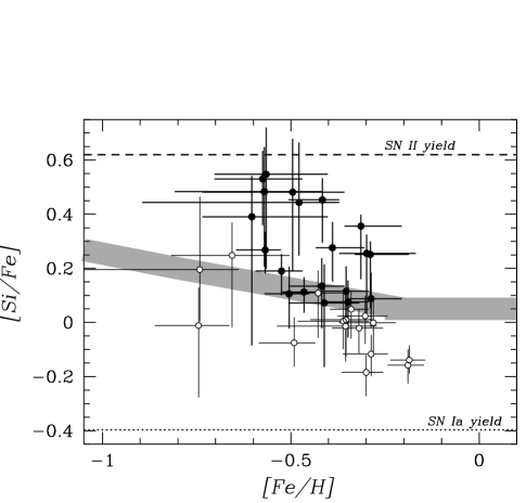
Figure 5.— [Ne/Fe] (left panel) and [Si/Fe] (right panel) vs [Fe/H] in clusters (filled circles) and groups (open circles). The thick gray line in the right panel shows the observed abundance pattern in Galactic stars and the thick gray line in the left panel shows the corresponding theoretical prediction for Ne (Timmes, Woosley and Weaver 1995). The thickness of the lines reflect the intrinsic scatter. Abundance units correspond to “meteoritic” values from Anders & Grevesse (1989) and [] indicates logarithmic values. Error bars are shown at the 68% confidence level. The dotted lines show our adopted SN Ia yield ratios and the dashed lines our adopted SN II yield ratios. The plots contain several points per system at different radii.

While the results for the S distribution in clusters are affected by uncertainties in the measurements, in general, global gradients in $\alpha$-process elements in our sample appear to be considerably weaker than the Fe abundance gradients. This has the direct implication that SN II products are more widely distributed in clusters, while SN Ia products are more centrally concentrated. According to the simulations of Metzler & Evrard (1994), much of the expected abundance gradient is due to different distributions between galaxies and gas. Within this scenario, the different distributions of SN Ia and SN II products can be explained if the radial behavior of gas-to-galaxy ratio differs between the main epochs of release of these products. SN II products should be released whilst galaxy and gas distributions are similar (resulting in weak abundance gradients), whilst later, when SN Ia products are released, the gas distribution should be more extended than that of the galaxies in order to reproduce the observed gradients. This picture is in general agreement with the findings of Ponman et al. (1999), that SN II-driven winds are mostly released before cluster collapse and preheat the gas. The resulting flattening of the gas profile, relative to the galaxy distribution, then leads naturally to the generation of an abundance gradient if further processed gas is injected from galaxies after the difference in density profiles has been established. We will return to the role of the different SN types in the metal enrichment process below.

4. Element Abundance Ratios

The radially increasing importance of SN II in the enrichment process of clusters is well illustrated in Fig.3.4, which shows how the Si/Fe abundance ratio varies with radius in groups and clusters. This figure shows that most rich clusters are characterized by an overabundance of Si relative to Fe at large radii relative to the solar ratio. At large radii, groups can attain gas mass fractions comparable to rich clusters (see below), but they still lack the metals in terms of lower Fe abundances and IMLRs (see Figs.1 and 5).

vs [Fe/H] in clusters of galaxies (filled circles) and in cD galaxies (open circles). The lines are the same as in Fig.5 (with the thick gray line representing the observed abundance pattern in Galactic stars).

We compare our abundance determinations for the hot gas in groups and clusters with stellar data in Fig.5. To make a direct comparison between the hot gas and stars, we convert our abundances to the “meteoritic” units in Anders & Grevesse (1989). We omit the data within the central 200 kpc of clusters where enrichment by cD galaxies may be important. Fig.5 shows that the gas in groups experienced a greater relative enrichment from SN Ia compared to the gas in rich clusters ($-0.2\pm 0.05$ dex in terms of [Si/Fe] for a given [Fe/H]). This can arise from either a greater release of SN Ia elements or a greater loss of SN II ejecta in groups compared with that in rich clusters. As we show below, the mass of heavy elements injected by SN Ia per unit blue luminosity is similar in groups and clusters; however, groups have a global deficit of SN II ejecta. Examination of Fig.5 shows that simply coadding groups will not reproduce cluster abundance ratios even in the high abundance central regions. Groups also lack the high Si/Fe component, seen in the outskirts of rich clusters.

Supersolar Si/Fe ratios found at the outskirts of clusters of galaxies can be considered as an evidence for a top-heavy IMF (Loewenstein & Mushotzky 1996; Wyse 1997). However, there is strong observational evidence in favor of a universal IMF (of the form characterized by Kroupa, Trout and Gilmore 1993), based on several different studies (cf Proc. of 33 ESLAB Symposium; Wyse 1997). So, as an alternative to suggestion of Loewenstein & Mushotzky (1996), we consider below a preferential loss of SNII ejecta. Our arguments assume a delay in SN Ia enrichment relative to SN II enrichment. As long as the escape of SN II ejecta occurs before SN Ia start to explode, than the observed Si/Fe ratio in IGM can be reproduced. Observations of our galaxy imply a time lag in SN Ia enrichment of $\sim 3$ Gyr (Yoshii et al. 1996).

According to theoretical modeling of SN Ia explosion, this delay results from low-metallicity inhibition of SN Ia (Kobayashi et al. 1999), so a delay in SN Ia enrichment in elliptical galaxies could be reduced to $\sim 0.1$ Gyr. We thus conclude that the enrichment of the IGM originates from either metal-poor galaxies or from short lived star bursts. Assuming the former, we can reproduce the high iron abundance in the ICM only via metal-rich galactic winds (but not e.g. by stripping of the gas), so star-bursts are required in both scenaria. Observations of cluster galaxies indicate a reduced star-formation activity (Balogh et al. 1998). Together with a flat radial distribution of $\alpha$-process elements this argues in favor of SN II enrichment occurring before cluster collapse. Since escape of SN Ia ejecta is enhanced at the end of the star burst (Recchi et al. 2000), detailed simulations are needed in order to justify the short-lived starburst scenario, proposed here.

As was shown by Mushotzky et al. (1996) and later confirmed by Finoguenov & Ponman (1999), the observed S/Fe ratios of clusters are consistent with pure SN Ia yields, despite the fact that S is an $\alpha$-process element. Fig.4 shows that our results reinforce this problem. Applying the results of SN II nucleosynthesis calculations to measurements of [S/Fe] vs [Fe/H] for galactic stars, Timmes, Woosley and Weaver (1995) conclude that sulfur is mainly produced by very massive progenitors ($M>30$$M_{\odot}$) of high metallicity (Fe abundance $>0.1$ solar). Thus, lack of S in ICM, argues in favor of production of bulk of elements in metal-poor galaxies. As discussed in Timmes et al. (1995), sulfur is not directly measured in stars or modeled with a high degree of certainty, but may serve to discriminate the flat IMF required to explain both cluster and elliptical enrichment. In addition, [S/Fe] in the ICM can provides constraints on the release of elements from spiral galaxies, which are expected to have high [S/Fe].

Alternatively, a non-spherical SN II explosion was proposed to explain the low S/Fe (Nagataki & Sato 1998). In this scenario it is possible to have the top-heavy IMF, and the production of sulfur in metal-rich galaxies together.

5. Iron Mass to Light ratios

The iron mass-to-light ratio (IMLR, in units of $h_{50}^{-1/2}$$M_{\odot}$/$L_{\odot}$) is a very useful diagnostic for characterizing the ability of a system to synthesize and retain heavy elements. Previous calculations of the IMLR were based on central iron abundance determinations, which can overestimate the cumulative IMLR within 3 Mpc by a factor of 3, assuming that that the Fe abundance drops to 0.1 solar at this radius. By resolving the spatial distribution of heavy elements, we can make a comparison with the distribution of optical light and not just the integrated values. The basic optical properties of our cluster sample are summarized in Table 1. The optical light is normalized to the observed value $L_{B}$ (col. 3 or col. 5 in Tab.1) within a radius $R_{L_{B}}$ (col. 4 in Tab.1 or 0.5 Mpc, when $L_{B}$ values are taken from col. 5), and a King profile is assumed for the galaxy light distribution. The cumulative IMLR, including light from the cD galaxy (which we include as a central point source) is shown in Fig.5. The radii in Fig.5 are expressed in units of the virial radius (see Tab. 1, col. 13).

Cumulative IMLR. The grey lines denote groups and black lines denote clusters. A2597 is omitted from the plot for clarity, however, due to the low optical luminosity of its cD galaxy, the corresponding IMLR is similar to Fig.7.

While the IMLR increases with radius in all systems, clusters have higher IMLR values at a given radius compared with that in groups. The IMLR is less than 0.02 at all radii in clusters and less than 0.006 at all radii in groups. In the central $\sim 70$ kpc of cD groups and clusters (this only excludes HCG51 and HCG62), the IMLR is less than 0.001. The Fe in this region can be produced by stellar mass loss from the cD galaxies alone (cf Mathews 1989).

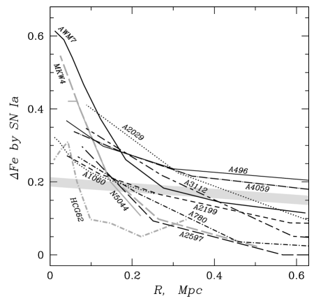
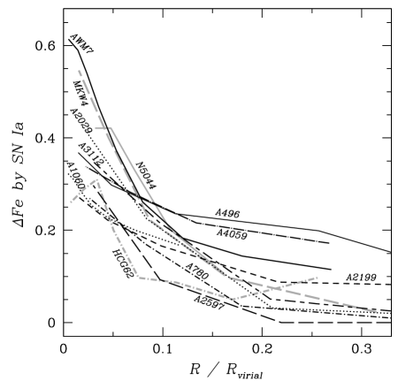
Figure 6.— $\Delta Fe$ (in solar ’photospheric’ units) injected by SN Ia as a function of radius (in units of Mpc in the left panel and virial radii in the right panel). Gray lines represent groups and black lines represent clusters. Error bars at all radii are on average 0.1 at 68% confidence level. The thick gray line shows the variation in the early-type galaxy fraction with radius in clusters (Whitmore, Gilmore and Jones 1993) adjusted by a factor of 0.2 for illustrative purposes. Comparing the two figures one can see that the scatter in the data is diminished when virial units are used.

5.1. IMLRs of both Types of SNe

By resolving the spatial distribution of elements synthesized in different types of SNe, we can determine the IMLR for each type. The primary method for discriminating between enrichment by SN Ia and SN II lies in the differences between their heavy element yields. This is primarily reflected in differences between the $\alpha$-process elements and Fe. In order to separate the input of different types of SN to the observed element distributions, we have to make assumption about SN yields. The heavy element yields of SN II were recently calculated by Woosley and Weaver (1995). Since then a major effort has been carried out to compare their yields with stellar data and observations of SN 1987A. These studies (e.g.  Timmes, Woosley and Weaver 1995; Prantzos and Silk 1998) indicate that the yields for the iron-peak elements in the Woosley and Weaver models should be reduced by a factor of $\sim 2$. This reduction is primarily driven by the observed O/Fe ratios in stars and observations of other $\alpha$-process elements including Si (Prantzos private communication). One of the main goals of this paper is to discriminate between the Fe that originated from the two types of supernovae. To accomplish this we adopt Si and Fe yields of $y_{Si}=0.133$$M_{\odot}$ and $y_{Fe}=0.07$$M_{\odot}$ for SN II. We note that $y_{Fe}=0.07$$M_{\odot}$ was also adopted in Renzini et al. (1993). The yields of SN Ia are obtained from Thielemann et al. (1993) with $y_{Si}=0.158$$M_{\odot}$ and $y_{Fe}=0.744$$M_{\odot}$. To decompose the Fe profiles into contributions from the two types of SNe, we use the observed Si and Fe abundances in each cluster and the adopted SN yields, as listed above. This approach has the advantage that Si and Fe abundance profiles have been determined for our entire sample, and that the spread in the Si yields is low between different modeling of SN element production (cf Gibson et al. 1997).

As can be seen in Fig.6, the contribution from SN Ia to Fe abundance is centrally concentrated in all systems. The [Fe/H] distribution from SN Ia depends on the spatial distribution of the injected Fe relative to the distribution of the ambient gas when the enrichment occurs. For example, if we assume that during the period of enrichment the gas and galaxies have the same distribution and that all galaxies contribute equally to the enrichment, then [Fe/H] would be independent of radius. Since a negative iron abundance gradient is observed, SN Ia enriched gas must be preferentially released near the center of groups and clusters.

In Fig.6 we also show the radial behavior of the early-type galaxy fraction in clusters (Whitmore et al. 1993). Whitmore et al. find this behavior to be universal in all clusters in their sample. We note however, that their sample only includes systems optically richer than A1060. Beyond the central 300-400 kpc, the radial variation in the early-type galaxy fraction is in good agreement with the declining iron abundance. In the central regions of the groups and clusters, however, the abundance of iron increases much faster than the early-type galaxy fraction. Fig.6 also shows that the scatter in SN Ia profiles inside the central $0.1R_{virial}$ is diminished when virial units are used instead of physical distances. These results indicate that the central concentration of SN Ia synthesized Fe cannot be explained by the increased fraction of early-type galaxies at cluster centers. Density dependent mechanisms (e.g. ram pressure stripping, galaxy harassment, and tidal disruption) are therefore favored.

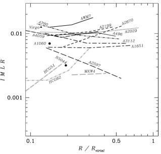
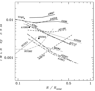
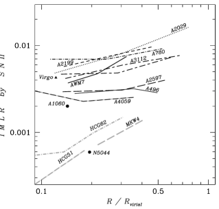
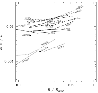
Figure 7.— M/L ratios for total Fe mass, Fe from SN Ia, Fe from SNII, and Si vs cluster radius in units of virial radii (left column). The middle and right columns show the same M/L ratios at fixed radii of $0.2R_{virial}$ and $0.4R_{virial}$. The central 200 kpc was omitted to exclude the effects of cD galaxies, except for HCG51 and HCG62 which do not contain cD galaxies.

Figure 8.— [Si/Fe] vs Si MLR (left panel) and [Si/Fe] vs. gas mass fraction (right panel). All values are evaluated at 20% of the virial radius. Dashed lines indicate the adopted SN II yields.

In the following analysis we exclude the central 200 kpc in the computation of the Fe mass and optical light. This allows us to include the IMLR for A780 and A1651 for which the luminosities of the cD galaxies are not available. This exclusion only leaves one remaining point for Virgo, A1060, and NGC5044. In Fig.7 we show the total IMLR, its decomposition into type II and Ia SN, and the Si M/L. This figure shows that Fe synthesized in SN Ia is centrally concentrated in groups and clusters, while Fe synthesized in SN II is dominant in the outer regions of clusters. The distribution of the Si M/L ratio is very similar to the Fe M/L ratio from type II SNe and is, on average, flat or increases slightly with radius. Clusters also have larger values of Si M/L than groups. The radial behavior of the Si M/L and Fe M/L from SN II profiles is consistent with the scenario in which SN II ejecta is only weakly retained (or captured) in groups.

We also show in Fig.7 how the IMLR varies with cluster temperature at radii of $0.2R_{virial}$ and $0.4R_{virial}$. At a given fraction of a virial radius, the IMLR from SN II and the Si M/L increases with gas temperature. This trend implies a greater retention ability of Fe and Si released by SN II in hotter systems. The average value of the IMLR from SN II among the clusters is 0.005 at 0.2$R_{virial}$ and 0.009 at 0.4$R_{virial}$.

Fig.8 shows how the Si/Fe abundance ratio varies with Si M/L and gas mass fraction at a fixed radius of 0.2$R_{virial}$. The large scatter in gas mass fraction in our analysis occurs at a much smaller radius than studied by Ettori & Fabian (1998) and Vikhlinin, Forman & Jones (1999) who observed very little scatter in the cluster gas mass fraction. These results are discussed in Finoguenov, Arnaud, David (2000) where we find that the scatter in gas mass fraction decreases strongly with radius, as the central entropy floor of a system becomes negligible compared to the total entropy of the system at large radii. As follows from Fig.8, systems that retained or accreted the most gas also have the largest Si M/L ratios and Si/Fe ratio representative of SN II ejecta. Finoguenov & Ponman (1999) came to a similar conclusion by examining the radial behavior of the IMLR and gas mass fraction in clusters. These arguments also provide strong constraints on the relative importance of AGNs in heating the cluster gas (Wu, Fabian and Nulsen 1999).

The Si/Fe ratio in groups and clusters varies by 0.8dex, fully spanning the range from pure SN Ia ejecta to pure SN II ejecta. In some clusters, contribution of SN Ia to element enrichment reaches 0.01 in terms of IMLR. Using the modeling of the cosmic history of SN Ia explosion (Tab.1 in Renzini et al. 1993) we conclude the role of SNe Ia in the iron enrichment process of the ICM is consistent with the present-day SN Ia rate found in optical searches (Capellaro et al. 1997) and the abundances determined from X-ray observations of early-type galaxies (cf Finoguenov & Jones 2000), but requires higher SN Ia rates in the past.

6. Summary

We have derived the distribution of heavy elements in a sample of groups and clusters and compared these distributions to the galaxy distribution. Our main results are:

• For clusters with the best photon statistics, we find that the total Fe abundance decreases significantly with radius, while the Si abundance is either flat or decreases slightly. This results in an increasing Si/Fe ratio with radius and implies a radially increasing predominance of type II SNe enrichment in clusters.

• SN Ia products show a strong central concentration in most clusters, suggesting an enrichment mechanism with a strong density dependence (e.g., tidal / ram pressure stripping of infalling gas rich galaxies). Moreover, the corresponding IMLR for SN Ia decreases with radius in most clusters.

• Our results strongly favor a model in which SNe II explode mostly before cluster collapse, whilst SNe Ia ejecta are removed from galaxies by e.g. a density-dependent mechanism after cluster collapse, in general agreement with the findings of Ponman et al. (1999). In simulations of the formation of abundance gradients this has not yet been taken into account.

  In a scenario suggested by the simulations of Metzler & Evrard (1994), flattening of the gas profile relative to the galaxy distribution will naturally produce an abundance gradient if the processed gas is injected after the difference in density profiles is established. Therefore this model should be applied only to the Fe contributed later by SN Ia. If this scenario is correct, the distribution of IMLR from SN Ia (as opposed to the Fe abundance) should be flat with radius, whilst if density-dependent mechanisms are at work, IMLR should decrease with radius. Given the radial behavior of the IMLR attributed to SN Ia (Fig.11), we suggest that both mechanisms may be important in the formation of the observed Fe abundance gradient.

• The dependence of [Si/Fe] vs [Fe/H] reveals a larger role of SN Ia in the enrichment of groups compared with that in clusters. Due to differences in the elemental abundance patterns, it is not possible to produce a cluster simply by coadding groups. The lack of metals attributed to SN II in groups suggests that SN II products were only weakly captured (or retained) by the shallower potential wells of groups due to the high entropy of the preheated gas.

• As an alternative to a top heavy IMF, we propose an explanation for the observed supersolar Si/Fe ratios involving preferential loss of SN II products from galaxies, arising from either very short duration star-bursts or from enrichment by metal-poor galaxies. Observations of subsolar S/Fe ratios argues in favor of the latter suggestion.

7. Acknowledgments

AF acknowledges support from Alexander von Humboldt Stiftung during preparation of this work. The authors acknowledge the devoted work of the ASCA operation and calibration teams, without which this paper would not be possible. We thank Monique Arnaud for communicating to us the idea regarding Si M/L ratio, Maxim Markevitch for his help in simulating the systematic effects of ASCA XRT PSF, Alexey Vikhlinin for allowing gas mass comparison with his ROSAT/PSPC results, and the referee for stimulating us to check the effects of systematics in our modeling and for a number of useful suggestions regarding theoretical interpretation of the data. Simulations required for this work were performed using computer resources of ISDC, CfA and AIP.

Appendix A Drawbacks of application to CCD-quality spectra of MEKAL modeling of the iron L-shell complex as an abundance indicator.

Discordant results have been reported for element abundance determinations using X-ray emission of early-type galaxies and galaxy groups. Supersolar metallicities have been derived by Buote (1999, 2000a), fitting two-temperature models to the integrated hot plasma emission from within the central regions of galaxies and groups. Lower metallicities are found using single-temperature models (e.g. Matsushita 1998), and also from spatially resolved single-temperature fits combining ROSAT and ASCA data (Finoguenov et al. 1999; Finoguenov and Ponman 1999; Finoguenov and Jones 2000).

Single-temperature models, when used to fit an intrinsically two-temperature plasma, can be shown to underestimate element abundances (Buote 1999; Finoguenov and Ponman 1999). However, real spectra from hot gas are unlikely to be two-temperature, and fitting two-temperature models can also give misleading results. Consider, for example, the following simple simulation: using a MEKAL model with kT=1.35, Z=0.33, $N_{H}=0.7\times 10^{21}$ (and other parameters as for HCG51), we simulate an ASCA SIS spectrum and then fit a two-temperature MEKAL model. The final reduced $\chi^{2}$ is about 2/3 instead of 1, and the abundance is biased high (0.4–0.6 in different runs, with varying exposure times). Now, when we have to fit the real spectra, the MEKAL code does not exactly match the source emission, due to the complex physics of iron L-shell emission. Recent high-energy resolution data has been used to benchmark the MEKAL code (Phillips et al. 1999), revealing at least 10% systematics for the CCD energy resolution, while mismatches in line positions will be a dominant problem at a resolution of few ev. Given the presence of such systematics, overfitting the spectrum with a two-temperature model may compensate for data-model mismatches, and give reduced $\chi^{2}$ values $\sim 1$.

Taking a more realistic case, we use our derived radial distributions of temperature and emission measure for HCG62, together with an iron abundance dropping from 0.5 solar at the center down to 0.2 solar at $r=$6^′. Comparing the integrated spectrum from this region with that from a two-temperature MEKAL model with parameters fixed at the values published by Buote (2000a), we find that the fit does not deviate from the simulated data by more than 10%, which is well within the systematic uncertainty of the MEKAL model. However, the Fe abundance in this model is solar, deviating by factors 2–5 from the abundance input into these simulations. The problem arises because Buote’s results are derived from spectral fits to integrated spectra from a region which is generally dominated by a central cooling flow.

In a more recent paper, Buote (2000b) has performed a spatially resolved spectral analysis of a number of the systems in our study using ROSAT PSPC data, this time employing single-temperature model fits. Again he finds extremely high central abundances in many of his systems – for example, his central Fe abundance for HCG62 lies in the range 5-15 solar, in strong conflict with our results. Buote (2000b) suggests that our low abundance determination at the center of HCG62 is due to ‘over-regularization’. Since it is certainly true that regularization would tend to suppress such a huge central spike in abundance, if observed at low statistical significance, we have checked the effect of completely turning off the regularization for Fe in our analysis of HCG62. The result can be seen in Fig.1. As expected, the abundance is subject to larger fluctuations, however, our basic results that the abundance is subsolar, and drops at large radii, are unchanged. In Finoguenov, Arnaud & David (2000) we have analyzed Centaurus cluster, which has a very steep abundance gradient profile and obtained similar results to Ikebe et al. (1999). In addition we have simulated and shown that an extremely peaked abundance profiles, e.g. 10 times solar as reported in Buote (2000b), could not remain unseen by our analysis if it were present.

To check the effects on our results of possible systematic effects of using the MEKAL code, we included a 10% systematic error into the fitting process and reanalyzed the ASCA observation of HCG62. This analysis naturally produces larger error bars in metallicity in the 0.1–0.4 Mpc region, permitting values up to 0.6 solar at 0.1 Mpc at the 90% confidence limit (previously 0.4) and up to 0.3 at 0.2 Mpc (previously 0.2). With the revised ASCA error estimates, the mild discrepancy between our ASCA result and the ROSAT Fe determinations reported in Finoguenov & Ponman (1999) (and shown in Fig.1) is removed. Also, a Si abundance of 0.35 solar is permitted at 0.4 Mpc (previously 0.25). We have also analyzed the 1998 ASCA observations of HCG62 as an independent check. Both ASCA sets of observations independently yield Fe abundance between 0.3 and 0.5 Mpc at the $0.15\pm 0.10$ level.

The conclusions that we draw from the above are that in the central cooling regions of groups and clusters the temperature structure may be complex at each radius, and also varies with radius. We believe that there is considerable doubt in the credibility of abundance determinations derived from integrated CCD-quality spectra of such regions using any modeling. Results derived from the lower spectral resolution spectra available from the ROSAT PSPC are even more suspect. Higher resolution X-ray spectra will be required to derive reliable results for such regions. At larger radii, where gas density is lower and cooling times long, it is reasonable to represent the gas as a single temperature plasma at each radius. In this regard it is encouraging that temperature distributions from ROSAT and ASCA analyses are generally in good agreement (Finoguenov & Ponman 1999, Finoguenov & Jones 2000). Here we believe that results from our analysis should be correct to within systematic uncertainties resulting from the use of the MEKAL model.

References

- (1) Allen S. and Fabian A. 1998, MNRAS, 297, 63
- (2) Anders E. and Grevesse N. 1989, Geochimica et Cosmochimica Acta, 53, 197
- (3) Arnaud M., Rothenflug R., Boulade O., Vigroux L. and Vangioni-Flam, 1992, A&A, 254, 49
- (4) Cappellaro E., Turatto M., Tsvetkov D., Bartunov O., Pollas C., Evans R. and Hamuy M. 1997, A&A, 322, 431
- (5) Balogh M., Schade D., Morris S., Yee H., Carlberg R., Ellingson E. 1998, ApJ (Letters), 504, L75
- (6) Bahcall N. 1981, ApJ, 247, 787
- (7) Beers T.C., Geller M.J., Huchra J.P., Latham D.W., Davis R.J. 1984, ApJ, 283, 33
- (8) Bird C. 1994, ApJ, 422, 480
- (9) Buote D., 1999, MNRAS, 309, 685
- (10) Buote D., 2000a, MNRAS, 311, 176
- (11) Buote D., 2000b, ApJ, submitted (astro-ph/0001329)
- (12) Burke B.E., Mountain R.W., Harrison D.C., Bautz M.W., Doty J.P., Ricker G.R. and Daniels P.J., 1991, IEEE Trans., EED-38, 1069
- (13) Churazov E., Gilfanov M., Forman W., Jones C., 1996, ApJ, 471, 673
- (14) David L., Forman W. and Jones C. 1991, ApJ, 369, 121
- (15) David L., Arnaud K., Forman W., Jones C. 1990, ApJ, 356, 32
- (16) Dell’Antonio I., Geller M., Fabricant D. 1995, AJ, 110, 502
- (17) D’Ercole A. and Brighenti F. 1999, MNRAS, accepted, (astro-ph/9907005)
- (18) De Young D. 1978, ApJ, 223, 47
- (19) Dupke R., White III R. 1999, ApJ, in press, (astro-ph/9907343)
- (20) Edge A. C. and Steward G. C., MNRAS, 1991, 252, 428
- (21) Ettori S. and Fabian A. 1999, MNRAS, 305, 834
- (22) Evrard A., Metzler C. and Navarro J. 1996, ApJ, 469, 494
- (23) Fabian A., Arnaud K., Bautz M., Tawara Y. 1994, ApJ, 436, 63
- (24) Finoguenov A., Jones C., Forman W. and David L., 1999, ApJ, 514, 844
- (25) Finoguenov A. and Ponman T., 1999, MNRAS, 305, 325
- (26) Finoguenov A. and Jones C., 2000, ApJ, accepted (astro-ph/0003202)
- (27) Finoguenov A., Arnaud M. and David L., 2000, ApJ, in preparation
- (28) Fukazawa Y., Makishima K., Tamura T., Ezawa H., Xu H. et al. 1998, PASJ, 50,187
- (29) Gibson B.K., Loewenstein M. and Mushotzky R.F. 1997, MNRAS, 290, 623
- (30) Girardi M., Biviano A., Giuricin G., Mardirossian F., Mezzetti M. 1995, ApJ, 438, 527
- (31) Gunn J.E. and Gott J.R., 1972, ApJ, 176, 1
- (32) Hobbs I.S. and Willmore A.P. 1997, MNRAS, 289, 685
- (33) Ikebe Y., Makishima K., Ezawa H., Fukazawa Y., Hirayama M., et al. 1997, ApJ, 481, 660
- (34) Ikebe Y., Makishima K., Fukazawa Y., Tamura T., Xu H., Ohashi T., Matsushita K. 1999, ApJ, 525, 58
- (35) Kikuchi K., Furusho T., Ezawa H., Yamasaki N., Ohashi T., Fukazawa Y., Ikebe Y., 1999, PASJ, 51, 301
- (36) Kobayashi C., Tsujimoto T., Nomoto K., Hachisu I., Kato M., 1998, ApJ, 503, 155
- (37) Kroupa P, Tout C., Gilmore, G. 1993, MNRAS, 262, 545
- (38) Liedahl D.A., Osterheld A.L. and Goldstein W.H. 1995, ApJ (Letters), 438, L115
- (39) Loewenstein M. and Mushotzky R.F. 1996, ApJ, 466, 695
- (40) Markevitch, M., Forman, W. R., Sarazin, C. L., & Vikhlinin, A. 1998, ApJ, 503, 77
- (41) Mathews W.G. 1989, AJ, 97, 42
- (42) Matsushita K. 1998, PhD thesis, University of Tokyo
- (43) Metzler C.A. & Evrard A.E. 1994, ApJ, 437, 564
- (44) Mewe R., Gronenschild E.H.B.M. and Oord G.H.J. 1985, A&A (Supplement Series), 62, 197
- (45) Mewe R. & Kaastra J. 1995, Internal SRON-Leiden report
- (46) Mitchell R., Ives J. and Culhane L., 1975, MNRAS, 175, 29
- (47) Mohr J., Mathiesen B. and Evrard A. 1999, ApJ, 517, 627
- (48) Mushotzky R.F., Loewenstein M., Arnaud K.A., Tamura T., Fukazawa Y., Matsushita K., Kikuchi K. and Hatsukade I. 1996, ApJ, 466, 686
- (49) Nagataki S., Sato K. 1998, ApJ, 504, 629
- (50) Phillips K., Mewe R., Harra-Murnion L., Kaastra J., Beiersdorfer P., Brown G., Liedahl D. 1999, A&A (Supplement Series), 138, 381
- (51) Ponman T.J., Cannon D.B., Navarro J.F. 1999, Nature, 397, 153
- (52) Prantzos N. and Silk J. 1998, ApJ, 507, 229
- (53) Press W.H., Teukolsky S.A., Vetterling W.T., Flannery B.P. 1992, Numerical recipes in FORTRAN
- (54) Recchi S., Matteucci F., D’Ercole A. 2000, MNRAS, submitted (astro-ph/0002370)
- (55) Renzini A., Ciotti L., D’Ercole A., Pellegrini S. 1993, ApJ, 419, 52
- (56) Renzini A. 1997, ApJ, 488, 35
- (57) Sarazin C., Wise M., Markevitch M. 1998, ApJ, 498, 606
- (58) Serlemitsos P. et al. , 1977, ApJ (Letters), 211, L63
- (59) Snowden S.L., McCammon D., Burrows D.N. and Mendenhall J.A. 1994, ApJ, 424, 714
- (60) Takahashi T., Markevitch M., Fukazawa Y., Ikebe Y., Ishisaki Y., et al. , 1995 ASCA Newsletter, no.3 (NASA/GSFC)
- (61) Tamura T., Day C., Fukazawa Y., Hatsukade I., Ikebe Y. et al. 1986, PASJ, 48,671
- (62) Tamura T., Makishima K., Fukazawa Y., Ikebe Y., Xu H., 2000, ApJ, accepted
- (63) Tanaka Y., Inoue H. and Holt S.S. 1984, PASJ, 46,L37
- (64) Thielemann F.-K., Nomoto K. & Hashimoto M. 1993 Origin and Evolution of the Elements. (ed. Prantzos N., Vangioni-Flam E. & Cassé M.). Cambridge Univ. Press, 297
- (65) Timmes F., Woosley S., Weaver T. 1995, ApJ (Supplement Series), 98, 617
- (66) Truemper J. 1983, Adv. Space Res., 2, 241
- (67) Vikhlinin A., Forman W., Jones C., 1999, ApJ, 525, 47
- (68) White R. 1991, ApJ, 367, 69
- (69) Whitmore B.C., Gilmore D.M. and Jones C. 1993, ApJ, 407, 489
- (70) Woosley S.E. and Weaver T.A. 1995, ApJ (Supplement Series), 101, 181
- (71) Wu K., Fabian A. and Nulsen P., 1999, MNRAS, in press (astro-ph/9907112)
- (72) Wise M. and Sarazin C. 1993, ApJ, 415, 58
- (73) Wyse R.F.G. 1997, ApJ, 490, L69
- (74) Yoshii Y., Tsujimoto T., Nomoto K. 1996, ApJ, 462, 266