Polarization fluctuations due to extragalactic sources

Abstract

We have derived the relationship between polarization and intensity fluctuations due to point sources. In the case of a Poisson distribution of a population with uniform evolution properties and constant polarization degree, polarization fluctuations are simply equal to intensity fluctuations times the average polarization degree. Conservative estimates of the polarization degree of the classes of extragalactic sources contributing to fluctuations in the frequency ranges covered by the forthcoming space missions MAP and Planck Surveyor indicate that extragalactic sources will not be a strong limiting factor to measurements of the polarization of the Cosmic Microwave Background.

1 Introduction

There are good prospects that the forthcoming space missions designed to provide high sensitivity and high resolution maps of the cosmic microwave background (CMB) will also measure the CMB polarization fluctuations (Knox 1998; Bouchet et al. 1999).

The current design of instruments for the Planck Surveyor mission (the third Medium-sized mission of ESA’s Horizon 2000 Scientific Programme) provides good sensitivity to polarization at all LFI (Low Frequency Instrument) frequencies (30, 44, 70, and 100 GHz) as well as at three HFI (High Frequency Instrument) frequencies (143, 217 and 545 GHz). The NASA’s MIDEX class mission MAP has also polarization sensitivity in all channels (30, 40 and 90 GHz).

The extraction of the very weak cosmological polarization signal requires both a great sensitivity of the instruments and a careful control of foregrounds. An analysis of the effect of Galactic polarized emissions (synchrotron and dust) on CMB measurements by the Planck and MAP missions was carried out by Bouchet et al. (1999). So far, however, the effect of extragalactic sources was not considered. On the other hand, significant linear polarization is seen in most compact, flat-spectrum radio sources which are the main contributors to small scale foreground intensity fluctuations at $\lambda>1\,$mm (Toffolatti et al. 1998) and the thermal dust emission from galaxies which dominate the counts at sub-mm wavelengths is also expected to be polarized to some extent, as the Galactic dust emission is observed to be (Hildebrand 1996).

In this paper we derive the relationship between intensity and polarization fluctuations in the case of a Poisson distribution of point sources, discuss the polarization degree of the relevant classes of extragalactic sources, and exploit recent evolutionary models to estimate the power spectrum of polarization fluctuations produced by them.

2 Polarization fluctuations from a Poisson distribution of polarized point sources

Following Burn (1966) we define the complex linear polarization of a source as $P_{s}=\Pi\exp(2i\chi)$ where $\Pi$ and $\chi$ are the degree and the angle of polarization, respectively. If the polarization angles of different sources within any given solid angle element $d\Omega$ are uncorrelated, the expected value $\langle P_{s}\rangle$ is 0 and the variance is:

$$\sigma^{2}_{P}={1/\pi}\int^{\pi}_{0}d\chi\,(P_{s}-\langle P_{s}\rangle)^{2}={1/\pi}\int^{\pi}_{0}d\chi\,\Pi^{2}\left[\cos^{2}(2\chi)+\sin^{2}(2\chi)\right]=\Pi^{2}.$$ (1)

Let $N=n(S)\,dS\,d\Omega$ be the number of sources with flux $S$ within $dS$ and polarization degree $\Pi$ in a given solid angle element $d\Omega$. As far as the central limit theorem holds, the expected value of the linear polarization within $d\Omega$ is also 0, with variance

$$\sigma^{2}_{P,{d\Omega}}={\Pi^{2}\over{N}}.$$ (2)

The fluctuation amplitude of the polarized flux $S_{P}={N}SP_{s}$ among the different cells of the sky subtending a solid angle $d\Omega$, due to sources with flux $S$, is therefore obtained integrating over the probability distribution of $N$, $\rho(N)$:

$$\sigma^{2}_{S_{P},d\Omega}=\langle\left(S_{P}-\langle S_{P}\rangle\right)^{2}\rangle=\langle S_{P}^{2}\rangle=\int_{0}^{\infty}d{N}\,\rho({N}){N}S^{2}\Pi^{2}=\Pi^{2}S^{2}\langle{N(S)}\rangle.$$ (3)

In the case of a Poisson distribution of sources the variance is equal to the mean. Therefore, integrating the above equation over $S$ and over the solid angle we straightforwardly obtain $\sigma_{I_{P}}=\Pi\sigma_{I}$, where $\sigma_{I}$ is the rms intensity fluctuation for a Poisson distribution of sources.

The assumption of an equal polarization degree for all sources is obviously unrealistic. However, it follows from the above calculations that, if the polarization degree is uncorrelated with flux, the result depends only on the mean value of $\Pi$.

A dependence of the mean value of $\Pi$ on $S$ arises, in particular, in the case of contributions from classes of sources with different polarization properties and different shapes of the $\log N$–$\log S$ curves. These different populations must be dealt with separately.

3 Linear polarization properties of the relevant classes of sources

Studies of the polarization properties of extragalactic sources at mm wavelengths are still scanty. Table 1 summarizes the main results on radio/mm sources. For each of the main source classes (in column 1) and for each wavelength in column 2, we give the median (column 3), the minimum (column 4) and the maximum (column 5) polarization value found in literature. Column 6 lists the references from which the reported values are derived.

Table 1: Radio and mm polarization measurements for extragalactic sources

	Band	Pmed	Pmin	Pmax	Reference
		(%)	(%)	(%)
BL Lac	4.8 GHz	3.6	1.5	7.5	Aller et al. 1999
	8.44 GHz	1.5	0.4	2.7	Marcha et al. 1996
	14.5 GHz	5.0	1.1	11.4	Aller et al. 1999
	$0.8-1.1$ mm	7.1	3.0	12.8	Nartallo et al. 1998
	$0.8-1.1$ mm	10.8	3.0	17.0	Stevens et al. 1996
FS QSO	$1.4-90$ GHz	2.5			Saikia & Salter 1988
HPQ	$0.8-1.1$ mm	7.4	4.6	10.5	Nartallo et al. 1998
LPQ	$0.8-1.1$ mm	4.9	2.1	7.9	Nartallo et al. 1998
FRII	1.4 GHz	$\sim$4			Saikia & Salter 1988
	1.4 GHz	$\sim$10	2.8	18.4	Ishwara-Chandra et al. 1998
	5 GHz	$\sim$6			Saikia & Salter 1988
	5 GHz	$\sim$10	2.4	18.2	Ishwara-Chandra et al. 1998
FRI	5 GHz	$\sim$7.5			Saikia & Salter 1988

As shown in Table 1, the three classes of objects (BL Lacs, QSOs and bright radio galaxies) emit almost the same fraction of polarized radiation in the radio band. The major extragalactic contributors to the non-thermal polarization at sub–mm and mm wavelengths are the flat spectrum (spectral index $\alpha\leq 0.5$ if $S_{\nu}\propto\nu^{-\alpha}$) compact radio sources (mainly BL Lacertae objects and flat spectrum QSOs). These objects constitute about 50% of the flux limited ($S>1$ Jy at 5 GHz) radio catalogue compiled by Kühr et al. (1981). Stickel et al. (1991) have drawn from this catalogue a complete sample of BL Lacertae objects brighter than $m=20$ mag. Out of it, we have selected a complete sub–sample of 14 objects ($RA>9^{h}$ and $\delta>0^{\circ}$), for which radio and/or mm polarization measurements are available.

The polarization data for objects in this sub-sample (hereinafter Stickel north) are listed in Table 2. The tabulated percentage polarization degrees were obtained averaging the measurements from long term monitoring programs. Data at 4.8 GHz, 8.1 GHz and 14.5 GHz are from Aller et al. (1985, 1999), those at 22 GHz, 31 GHz and 90 GHz are from Rudnick et al. (1985) and those at 1.1 mm are from Nartallo et al. (1998).

Table 2: Fractional Polarization Measurements for the Stickel north BL Lac Sample at several frequencies (GHz)

name	P(4.8)	P(8.1)	P(14.5)	P(22)	P(31)	P(90)	P(272)	z
	(%)	(%)	(%)	(%)	(%)	(%)	(%)
0954+658	7.5	$-$	6.0	$-$	$-$	$-$	$-$	0.367
1147+245	2.4	3.3	4.6	$-$	$-$	$-$	$-$	–
1308+326	2.3	2.5	3.0	5.6	5.3	2.0	9.9	0.997
1418+546	1.9	2.4	2.6	$-$	$-$	5.3	$-$	0.152
1538+149	4.9	5.8	7.5	$-$	$-$	$-$	$-$	0.605
1652+398	1.7	3.1	3.0	$-$	$-$	$-$	$-$	0.033
1749+096	3.1	3.3	3.4	6.5	$-$	5.5	5.6	0.320
1749+701	3.6	5.6	8.1	$-$	$-$	$-$	$-$	0.770
1803+784	3.1	3.0	3.9	$-$	$-$	$-$	$-$	0.684
1807+698	2.1	4.1	2.5	$-$	$-$	$-$	$-$	0.051
1823+568	4.3	5.9	5.8	$-$	$-$	$-$	$-$	0.664
2007+777	3.0	5.1	7.1	$-$	$-$	$-$	$-$	0.342
2200+420	5.0	3.6	5.2	0.8	3.2	4.3	8.1	0.069
2254+074	6.3	$-$	11.4	$-$	$-$	$-$	$-$	0.190

We have compared the average polarization percentages at the various wavelengths of sources in the Stickel north sample and in the sample by Aller et al. (1999), excluding those in common with the Stickel north sample. The agreement is very good (see Fig. 1). The mean polarization percentages (P_m), the 68% confidence uncertainties ($\Delta P_{m}$) obtained from the Student’s $t$ distribution ($\Delta P_{m}=t_{\nu}(0.32)\sigma_{P}\,(N-1)^{-1/2}$, where $N$ is the number of sources in the bin and $\nu=N-1$) and the dispersions, $\sigma_{P}$, for the Stickel north sample are given in Table 3.

Table 3: Average Polarization Percentages for Stickel north Sample

$\lambda$	$\nu$	Pm	$\Delta P_{m}$	$\sigma_{P}$	N
(cm)	(GHz)	(%)	(%)	(%)
6.25	4.80	3.66	0.49	1.74	14
3.70	8.10	3.98	0.40	1.29	12
2.07	14.5	5.29	0.73	2.57	14
1.36	22.0	4.30	2.83	3.06	3
0.97	31.0	4.25	2.69	1.48	2
0.33	90.0	4.28	1.10	1.60	4
0.11	272	7.87	2.00	2.16	3

Since for most objects in the two samples redshift information is available, we have converted the observed into the rest–frame wavelengths and computed the average polarization degrees in wavelength bins. The results for the Stickel north sample are given in Table 4 and plotted in Figure 1$b$, where the results for the Aller sub-sample are also reported for comparison. Table 4 gives the adopted wavelength intervals, the average $\lambda$ in each interval, computed as the geometric mean of the two wavelength limits, the average polarization fraction with its 68% confidence uncertainty from the Student’s $t$ distribution and its dispersion, and the number of available measurements in each wavelength interval.

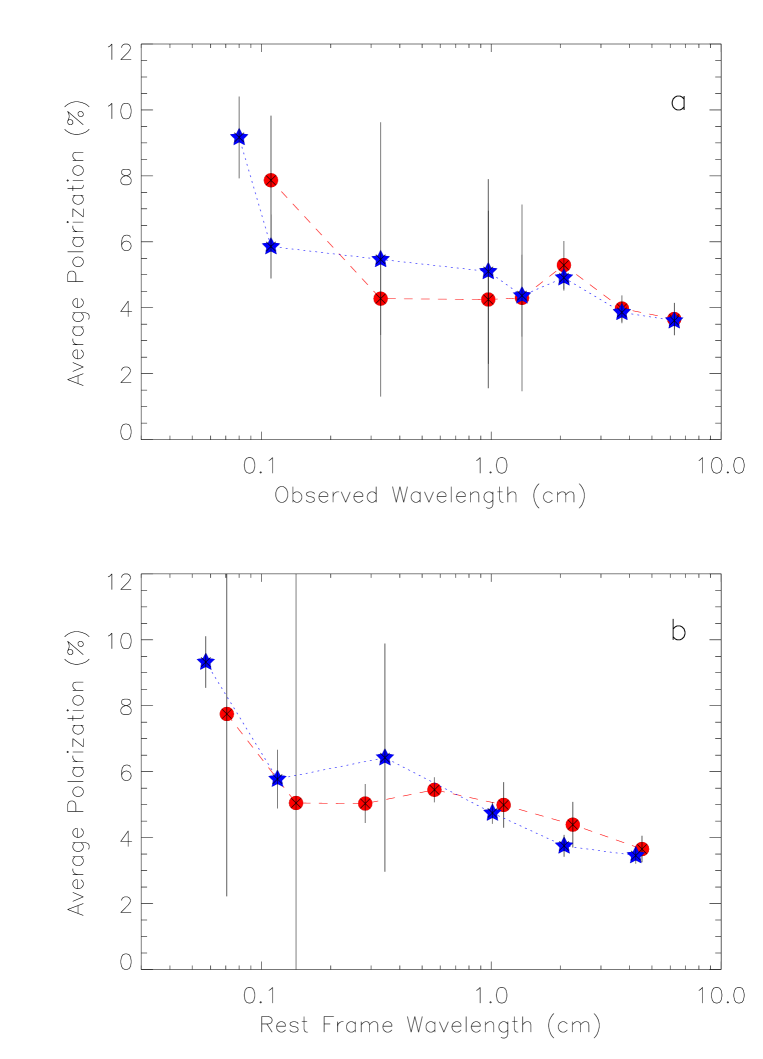
Figure 1: Average fractional polarization as a function of wavelength for two samples of BL Lac objects: red filled circles connected by the red dashed line stand for the Stickel north sample, while the blue filled stars connected by the blue dotted line stand for the the 28 sources in the Aller et al. (1999) sample that are not included in the Stickel north sample. The error bars correspond to the 68% confidence uncertainties on the estimated mean polarization.

Table 4: Average rest-frame polarization percentage for the Stickel north sample

$\Delta\lambda$	$\lambda_{m}$	Pm	$\Delta P_{m}$	$\sigma_{P}$	N
(cm)	(cm)	(%)	(%)	(%)
3.20–6.40	4.52	3.65	0.40	1.57	17
1.60–3.20	2.26	4.39	0.69	2.43	14
0.80–1.60	1.13	4.99	0.69	2.19	12
0.40–0.80	0.57	5.45	0.38	0.21	2
0.20–0.40	0.28	5.03	0.59	0.64	3
0.10–0.20	0.14	5.05	7.83	4.31	2
0.05–0.10	0.07	7.75	5.53	3.04	2

Measurements of polarized thermal emission from dust are only available for interstellar clouds in our own Galaxy. The distribution of observed polarization degrees of dense clouds at 100$\,\mu$m shows a peak at $\sim 2\%$ (Hildebrand 1996). The polarization degree of emission of silicate grains in clouds opaque to visible light but optically thin in the far-IR is nearly independent of wavelength if $\lambda\gg a$, $a$ being the grain size (Hildebrand 1988). This condition is very likely to be met at the long wavelengths of interest here.

Polarization maps of the Orion molecular cloud at $100\,\mu$m, $350\,\mu$m, $450\,\mu$m, $1.3\,$mm, and $3.3\,$mm (Schleuning 1998; Rao et al. 1998) look very similar except at clumps of higher optical depth, where the polarization increases with wavelength. In fact, the maximum polarization decreases rapidly with increasing optical depth (Hildebrand 1996); thus, the mm/sub-mm polarization may be higher than at $100\,\mu$m. On the other hand, the overall polarization of the light from a galaxy is the average of contributions from regions with different polarizing efficiencies and different orientations of the magnetic field with respect to the plane of the sky; all this works to decrease the polarization level in comparison with the mean of individual clouds.

We could not find any published polarization measurement of dust emission in external galaxies not hosting strong nuclear activity. However, the first results of the SCUBA Polarimeter include imaging polarimetry of the starburst galaxy M 82 at 850$\,\mu$m with a 15” beam size; a polarization degree of about 2% was measured (J. Greaves, private communication). An early image, available at the polarimeter Web page (http://www.jach.hawaii.edu/JCMT/scuba/scupol/
general/m82_polmap.gif), shows very ordered polarization vectors over scales of a few hundred parsecs. This may not occur in general. We may expect that, in other galaxies, the polarization vectors from giant molecular clouds are randomly ordered and tend to cancel out.

Polarimetric measurements at $170\,\mu$m with ISOPHOT have been carried out for two galaxies (U. Klaas, private communication): NGC 1808 (P.I.: E. Krügel) and NGC 6946 (P.I.: G. Bower). The results, however, are not available yet.

4 Power spectrum of polarization fluctuations due to extragalactic sources

Figure 2: Power spectra of CMB brightness temperature (thick solid line) and polarization fluctuations ($E$-mode: long dashes; $B$-mode: three dots/dash) compared with foreground polarization fluctuations at Planck/LFI frequencies. Following Tegmark & Efstathiou (1996) we plot the quantity $\delta T_{\ell}(\nu)=[\ell(2\ell+1)C_{\ell}(\nu)/4\pi]^{1/2}$. The thick dot-dashed and dashed lines correspond to synchrotron and interstellar dust emissions, respectively. The thin solid and dashed lines show our estimated contributions from extragalactic radio and far-IR sources, respectively, based on the model by Toffolatti et al. (1998), as updated by De Zotti & Toffolatti (1999). The thin dotted lines represent the expected noise spectrum per resolution element, averaged over the sky, of Planck/LFI. The heavier dots show the average MAP noise spectrum per resolution element at 30, 40 and 90 GHz.

Figure 3: Power spectra of polarized components at Planck/HFI frequencies with sensitivity to polarization. The lines have the same meaning as in Fig. 2. We show estimates of polarization fluctuations due to dusty galaxies (thin dashed lines) based both on model E by Guiderdoni et al. (1998; upper line) and on the model by Toffolatti et al. (1998).

In Figures 2 and 3 the power spectrum of foreground polarization fluctuations for all the relevant Planck and MAP channels is compared with the power spectrum of CMB anisotropies and of CMB polarized components. As for the latter, we have plotted the power spectra of the combinations of Stokes parameters defined by Seljak [1997; his eqs. (24) and (25)] and called $E$ and $B$. The estimate of $E$-mode polarization fluctuations refer to a standard CDM model (scale-invariant scalar fluctuations in a $\Omega=1$, $\Lambda=0$ universe with $H_{0}=50\,\hbox{km}\,\hbox{s}^{-1}\,\hbox{Mpc}^{-1}$ and a baryon density $\Omega_{b}=0.05$). The quantity $B$ vanishes for polarization induced by primordial scalar perturbations, and therefore provides a unique signature of tensor perturbations (Seljak 1997). The $B$-mode power spectrum shown in Figs. 2 and 3 refer to a tilted CDM model with power law indices $n_{s}=0.9$ and $n_{t}=n_{s}-1=-0.1$ for scalar and tensor perturbations, respectively; the other cosmological parameters keep the same values adopted for the standard CDM model. Calculations of CMB power spectra have been carried out using the CMBFAST package by Seljak & Zaldarriaga (1996).

The thick dashed lines show the $E$-mode of dust polarized power spectrum derived by Prunet et al. (1998), scaled to the central frequencies of Planck polarized channels using the dust emission spectrum adopted by these Authors (emission $\propto\nu^{2}B_{\nu}(17.5\,\rm{K})$, where $B_{\nu}(T)$ is the Planck function at frequency $\nu$ and temperature $T$).

The $B$-mode dust power spectrum turns out to be close to the $E$-mode one [cf. eqs (11) and (12) of Prunet et al. (1998)]. In fact, Seljak (1997) argued that most foregrounds should contribute on average the same amount to both modes. Therefore, for all foregrounds we consider a single polarized power spectrum, assumed to be representative of both modes.

Following Bouchet et al. (1999), we assume that, at all frequencies relevant for Planck and MAP, the synchrotron polarized emission is perfectly correlated with the total synchrotron emission (for which a power spectrum $C_{T}=4.5\ell^{-3}\,(\mu\rm{K})^{2}$ at 100 GHz was adopted) and the polarization degree is 44%. An antenna temperature spectral index of 3 ($T_{\rm A,syn}\propto\nu^{-3}$) has been used to extrapolate the power spectrum (in terms of brightness temperature) to the other Planck/MAP frequencies (see De Zotti et al. 1999 for references).

The polarized angular power spectra of extragalactic radiosources (thin solid lines) is estimated exploiting the model of Toffolatti et al. (1998), as updated by De Zotti & Toffolatti (1999). We have assumed that the mean polarization degree of BL Lacs in the Stickel north sample applies to all radio galaxies contributing to fluctuations in Planck’s channels; based on the results shown in Fig. 1, we have adopted a polarization degree of 5% for $\nu\leq 143\,$GHz, of 6% at 217 GHz and of 10% at 545 GHz.

As for dusty galaxies (thin dashed lines), we have adopted a polarization degree of 2% at all frequencies and the power spectra of temperature fluctuations derived by Toffolatti et al. (1998) and, for HFI channels, also by Guiderdoni et al. (1998; their model E).

A flux cut at 1 Jy was adopted for all channels (i.e. sources brighter than 1 Jy were removed); at 30, 100 and 217 GHz we show also the angular power spectrum derived adopting a flux cut of 100 mJy for radiosources (lower thin solid lines).

In Table 5 we report the values of $C_{\ell}$ for temperature fluctuations due to a Poisson distribution of extragalactic radio sources and dusty galaxies for the same cases shown in Figs. 2 and 3. The corresponding values for polarization fluctuations follow immediately multiplying by $\Pi^{2}$. Note that a Poisson distribution generates a simple white noise spectrum with the same power on all multipoles (Tegmark & Efstathiou 1996). The values of $C_{\ell}$ are given in terms of brightness temperature fluctuations and expressed in $\mu$K².

Table 5: Values of $C_{\ell}$ ($\mu$K²)¹ for temperature fluctuations for the cases shown in Figs. 2 and 3

$\nu$ (GHz)	30	44	70	100	143	217	545
$S_{l}$ = 1 Jy
Radiosources	$5.0(-2)$	$1.5(-2)$	$3.2(-3)$	$0.9(-3)$	$2.5(-4)$	$9.5(-5)$	$5.6(-3)$
(Toffolatti)
Far-IR sources	$1.5(-4)$	$4.0(-5)$	$7.6(-6)$	$3.1(-6)$	$2.8(-6)$	$1.0(-5)$	$3.0(-1)$
(Toffolatti)
Far-IR sources					$5.4(-5)$	$2.5(-4)$	$8.8(-1)$
(Guiderdoni)
$S_{l}$ = 100 mJy
Radiosources	$1.0(-2)$			$1.0(-4)$		$1.2(-5)$
(Toffolatti)
Far-IR sources	$5.0(-5)$			$1.5(-6)$		$6.0(-6)$
(Toffolatti)
Far-IR sources						$2.0(-4)$
(Guiderdoni)
1 In parenthesis are the powers of 10 (i.e. $5.0(-2)=5.0\,10^{-2}$)

As expected, polarization fluctuations due to extragalactic sources are particularly relevant at small angular scales. For multipoles $\ell\,\lower 2.0pt\hbox{${>\atop\hbox{\raise 4.0pt\hbox{$\sim$}}}$}\,300$, they in fact dominate foreground contributions at $\nu\,\lower 2.0pt\hbox{${<\atop\hbox{\raise 4.0pt\hbox{$\sim$}}}$}\,100\,$GHz. On these scales, at the lowest Planck frequency (30 GHz) their amplitude is, according to our estimate, close to that of CMB polarization fluctuations induced by scalar perturbations. In the “cosmological window” ($70\,\lower 2.0pt\hbox{${<\atop\hbox{\raise 4.0pt\hbox{$\sim$}}}$}\,\nu\,\lower 2.0pt\hbox{${<\atop\hbox{\raise 4.0pt\hbox{$\sim$}}}$}\,200\,$GHz), however, extragalactic sources are not seriously detrimental to measurements of CMB polarization fluctuations.

The thin dotted lines in Figs. 2 and 3 show the expected power spectra of instrumental noise, for polarization measurements, averaged over the sky, for Planck’s LFI and HFI, respectively. Following Tegmark & Efstathiou (1996) we describe the noise power spectrum as $C_{\ell,{\rm noise}}=\sigma^{2}{\rm FWHM}^{2}\exp(\ell^{2}\sigma_{b}^{2})$ where FWHM in expressed in radians, $\sigma_{b}={\rm FWHM}/2\sqrt{2\ln(2)}$ and $\sigma$ is the rms noise for a square pixel with side FWHM.

For LFI we have adopted the sensitivities for brightness temperature measurements given by Mandolesi et al. (1998) multiplied by a factor of 2 (Mandolesi, private communication). Sensitivities of HFI channels for polarization measurements are given by Puget et al. (1998). There is a slight difference in the mission duration adopted by the two groups to derive their mean sensitivity estimates: 12 months for LFI, 14 months for HFI.

The heavier dots in Fig. 2 show the expected mean instrumental noise per resolution element for MAP’s polarization measurements at 30, 40 and 90 GHz obtained from sensitivities for brightness temperature measurements (see the MAP Web page) multiplied by a factor $\sqrt{2}$ (G. Hinshaw, private communication).

As shown by Figs. 2 and 3, the major hurdle in extracting the CMB polarization signal is instrumental noise. However, a simple argument shows that, at least for a limited band-power range, sufficient sensitivity can be reached. We have investigated, in particular, the potential of LFI in this respect. The expected sensitivities to polarization per resolution element, averaged over the sky, for a 12 months mission, are 6, 10, 14 and 17$\,\mu$K at 30, 44, 70, and 100 GHz, respectively; the angular resolutions (FWHM) are 33’, 23’, 14’, and 10’, respectively (Mandolesi et al. 1998). Simulations done by C. Burigana indicate sensitivities 7 times better over areas of about 25 square degrees around each of the ecliptic poles. Within these areas, by rebinning the maps at 44, 70 and 100 GHz (we leave aside the 30 GHz map which is the most contaminated by polarized foregrounds) to a $\simeq 20^{\prime}$ resolution and combining them, a sensitivity to polarization of about $1\,\mu$K can be achieved, allowing to image the CMB polarization induced by scalar perturbations predicted by the standard CDM model. Of course, a lower sensitivity is enough to determine the first moments of the distribution of polarization fluctuations.

5 Conclusions

We have shown that the polarization fluctuations due to a Poisson distribution of point sources with uniform evolutionary properties and constant polarization degree are simply equal to intensity fluctuations times the average polarization degree.

The information on the polarization degree of the classes of extragalactic sources expected to dominate in the frequency ranges relevant for the MAP and Planck missions is scanty. We have taken a conservative approach, assuming that all radio sources are as polarized as BL Lac objects and that the polarization degree of dusty galaxies is similar to that of dense clouds in our own Galaxy and of M 82, a galaxy showing a remarkably ordered magnetic field.

We find that, on small scales (multipoles $\ell\,\lower 2.0pt\hbox{${>\atop\hbox{\raise 4.0pt\hbox{$\sim$}}}$}\,300$), polarization fluctuations due to radio sources may indeed dominate foreground contributions at $\nu\,\lower 2.0pt\hbox{${<\atop\hbox{\raise 4.0pt\hbox{$\sim$}}}$}\,100\,$GHz. However, in the “cosmological window” ($70\,\lower 2.0pt\hbox{${<\atop\hbox{\raise 4.0pt\hbox{$\sim$}}}$}\,\nu\,\lower 2.0pt\hbox{${<\atop\hbox{\raise 4.0pt\hbox{$\sim$}}}$}\,200\,$GHz), extragalactic sources are not a threat for measurements of CMB polarization fluctuations.

We have also argued that Planck/LFI can reach, in regions around the Galactic polar caps, polarization sensitivities of $\simeq 1\,\mu$K, allowing to map CMB polarization fluctuations on scales $\sim 20^{\prime}$. A detailed analysis of Planck and MAP capabilities for CMB polarization measurements has been carried out by Bouchet et al. (1999).

References

- [1] Aller H.D., Aller M.F., Latimer G.E. & Hodge P.E., ApJS 59 (1985) 513.
- [2] Aller M.F., Aller H.D., Hughes P.A. & Latimer G.E., ApJ 512 (1999) 601.
- [3] Bouchet F.R., Prunet S. & Sethi S.K., MNRAS, 302 (1999) 663.
- [4] Burn B.J., MNRAS 133 (1966) 67.
- [5] De Zotti G. & Toffolatti L., The CMB and the Planck Mission Proc. Santander Workshop (1999) in press.
- [6] De Zotti G., Toffolatti L., Argüeso F., Davies R.D., Mazzotta P., Partridge R.B., Smoot G.F. & Vittorio N., Proc. “3K Cosmology: EC-TMR Conference”, L. Maiani, F. Melchiorri, and N. Vittorio eds., AIP Conf. Proc. (1999) 204.
- [7] Ishwara-Chandra C.H., Saikia D.J., Kapahi V.K. & McCarthy P.J., MNRAS 300 (1998) 269.
- [8] Hildebrand R.H., QJRAS 29 (1988) 327.
- [9] Hildebrand R.H., Polarimetry of the Interstellar Medium W.G. Roberge & D.C.B. Whittet eds., ASP Conf. Ser. Vol. 97 (1996) 254.
- [10] Knox L., astro-ph/9811358 (1998).
- [11] Kühr H., Witzel A., Pauliny-Toth I.I.K. & Nauber U., A&AS 45 (1981) 367.
- [12] Mandolesi N., et al., Low Frequency Instrument for Planck. A proposal to the European Space Agency (1998).
- [13] Marcha M.J.M., Browne I.W.A., Impey C.D. & Smith P.S., MNRAS 281 (1996) 425.
- [14] Nartallo R., Gear W.K., Murray A.G., Robson E.I., Hough J.H., MNRAS 297 (1998) 667.
- [15] Prunet S., Sethi S.K., Bouchet F.R., Miville-Deschênes M.-A., A&A 339 (1998) 187.
- [16] Puget J.-L., et al.,High Frequency Instrument for the Planck mission. A proposal to the European Space Agency (1998).
- [17] Rao R., Crutcher R.M., Plambeck R.L., Wright M.C.H., ApJ 502 (1998) L75.
- [18] Rudnick L., Jones T.W., Aller H.D., Aller M.F., Hodge P.E., Owen F.N., Fiedler R.L., Puschell J.J. & Bignell R.C., ApJS 57 (1985) 693.
- [19] Saikia D.J. & Salter C.J., ARAA 26 (1988) 93.
- [20] Schleuning D.A., ApJ 493 (1998) 811.
- [21] Seljak U., ApJ 482 (1987) 6.
- [22] Seljak U. & Zaldarriaga M., ApJ 469 (1996) 437.
- [23] Stevens J.A., Robson E.I. & Holland W.S., ApJL 462 (1996) 23.
- [24] Stickel M., Padovani P., Urry C.M., Fried J.W. & Kühr H., ApJ 374 (1991) 431.
- [25] Tegmark M. & Efstathiou G., MNRAS 281 (1996) 1297.
- [26] Toffolatti L., Argüeso-Gómez F., De Zotti G., Mazzei P., Franceschini A., Danese L., Burigana C., MNRAS 297 (1998) 117.