Domain wall dominated universes

Abstract

We consider a cosmogony with a dark matter component consisting of a network of frustrated domain walls. Such a network provides a solid dark matter component with $p=-(2/3)\rho$ that remains unclustered on small scales and with $\Omega_{\rm dw}\approx 0.7$ can reconcile a spatially flat universe with the many observations indicating $\Omega_{\rm m}\approx 0.3.$ Because of its large negative pressure, this component can explain the recent observations indicating an accelerating universe without recourse to a non-vanishing cosmological constant. We explore the viability of this proposal and prospects for distinguishing it from other kinds of proposed dark matter with significant negative pressure.

Recent observations of apparent luminosities of Type Ia supernovae (SNIa) at moderate redshift $(\langle z\rangle\approx 0.6)$ suggest that the expansion of the universe is now accelerating, indicating a form of matter with a significant negative pressure [1]. From a theoretical standpoint, these observations are remarkable because most conceivable contributions to the stress-energy entail a positive (radiation) or vanishing (matter) pressure, rather than a large negative pressure.

Two proposals to explain these observations are a non-vanishing cosmological constant $(\Lambda)$ or a very slowly rolling scalar field, often dubbed quintessence. Both proposals, however, are plagued with formidable fine tuning problems. The fine tuning problems of $\Lambda\neq 0$ are well known [2]. For the alternative of a slowly rolling scalar field [3] extraordinarily flat potentials are required, so that the field is unable to roll to the true minimum by the present day. If the necessary flatness of such a potential is characterized by a mass scale $m$, one requires $m\sim 10^{-33}~{}{\rm eV}$.

In this letter we suggest another form of dark matter with significant negative pressure—a solid dark matter (SDM) component with the properties of a relativistic solid [4]. The term solid here denotes a substance with a harmonic, non-dissipative resistance to pure shear (volume preserving) deformations. A perfect fluid with negative pressure ($w=p/\rho<0$) would have an imaginary sound speed, indicating instabilities most severe on the smallest scales. For a solid, however, with a sufficiently large shear modulus these instabilities are removed. Since the sound speed of perturbations of the solid should comprise a substantial fraction of the speed of light, its Jeans length today is comparable to the size of the current horizon, and hence an SDM component would remain unclustered on the smaller scales over which $\Omega_{\rm m}$ is measured and thus evade detection.

To compute the effect of an exotic dark matter component on the evolution of cosmological perturbations, more is required than just knowing how $w$ evolves throughout cosmic history [5]. As we will see, it is possible to construct dark matter components for which $w$ agrees at all times, but which respond differently to cosmological perturbations. Because of the non-vanishing shear modulus in the SDM case, large anisotropic stresses are generated, whereas in models with a $\Lambda\neq 0$ or a slowly rolling scalar field these stresses vanish. Furthermore, long-wavelength gravity waves entering the horizon at late times acquire an effective mass because of the energetic cost associated with pure shear deformations of spacetime. In a previous paper [4] two of us (MB and DNS) developed a formalism for computing the evolution of cosmological perturbations in the presence of a SDM component and computed the cosmic microwave background (CMB) anisotropy on large scales. Here we discuss the viability of such scenarios for creating cosmic structure and the prospects for distinguishing SDM from other types of dark matter with significant negative pressure using future measurements of the CMB. A subsequent paper [6] will elucidate in more detail the differences between these scenarios and other models, such as quintessence and $\Lambda\neq 0.$

A possible microphysical origin for SDM is a frustrated network of topological defects, either cosmic strings or domain walls (see ref. [7] for a review of cosmic defects). The standard picture for the formation and evolution of topological defects is that of a random network of defects produced in a cosmological phase transition which then evolves toward a self-similar scaling regime with the number of defects within a Hubble volume approaching a fixed number [8]. However, such behavior relies on the ability of the defects to untangle and lose energy essentially as fast as allowed by causality, and in more complicated models this need not occur. In particular, in theories with several species of defects or with non-Abelian symmetries, topological obstructions to such untangling may arise [9] and defect-dominated evolution can occur. The basic features of such evolution would be that after the decay of an initial transient the number of defects per co-moving volume approaches a constant[10, 11]. For the simple domain walls of most interest here this implies an equation of state with $w=-2/3$ ($\rho_{\rm dw}\sim a^{-1}$) and for strings $w=-1/3$ ($\rho_{\rm str}\sim a^{-2}$), although other values of $w$ may be possible as well. Simulations of non-Abelian cosmic strings [11] indicate behavior leading to a string-dominated universe and simulations of domain walls [13] find that the density of walls in a model with several vacua falls less rapidly than would be required by scaling. In axion models, where an additional symmetry breaking $U(1)\to Z_{N}$ allows for $N$ domain walls to meet at a string, scaling behavior has been observed [12]. The precise criterion for when defect domination takes place is not clear at present, although it seems clear that such models can exist. This is currently under investigation.

The symmetry breaking scale $\eta$ required for the formation of a network of frustrated domain walls with $\Omega_{\rm dw}\sim 1$ today is around $\eta\approx 100~{}{\rm KeV}$, assuming a phase transition at $T\approx\eta$, with initially one wall per horizon volume and a network immediately settling down to an equilibrium configuration which is subsequently swept along by the Hubble flow. This estimate, however, is subject to considerable uncertainties in either direction. For example, a long transient before settling down to an equilibrium configuration could considerably raise $\eta$. The mean separation between walls is approximately 30 parsecs, much smaller than the scale on which the network clusters in response to gravitational perturbations. It is therefore justified to treat the network as a continuum solid when studying its response to cosmological perturbations.

In a recent article [14] it was suggested that a quintessence model with a flat geometry $w\approx-2/3$, $\Omega_{\rm c}=0.25$, $\Omega_{\rm b}=0.05$, $h=0.65$, $n=1$ gave a adequate fit to data probing a range of epochs and scales, where $\Omega_{\rm X}$ is the fractional density relative to the critical density in particle species X (X=c is CDM, X=b is baryons), the Hubble constant is $H_{0}=100h~{}{\rm km}\,{\rm sec}^{-1}\,{\rm Mpc}^{-1}$ and $n$ is the spectral index of the initial density perturbations. One might, therefore, wonder whether a domain wall dominated model with $\Omega_{\rm dw}\approx 0.7$ might fit the data equally well and, in fact, a number of the calculations presented in ref. [14] apply equally well to the case of a SDM model. However, important differences in how perturbations evolve once the SDM component comes to dominate must be considered for an accurate comparison to the data. Due to the apparently good fit of the $w=-2/3$ case, most of the discussion focuses on the domain wall dominated case, but we also discuss the string dominated case and other values of $w$. Except where expressly stated, all our results use the parameter choices listed above.

FIG. 1.: Rescaled CMB Moments for SDM Models. In the first four panels $\ell(\ell+1)C_{\ell}$ versus $\ell$ is plotted for $w=-1/3,-1/2,-2/3,-5/6$ for several values of the longitudinal sound speed for a universe with $\Omega_{\rm m}=0.3,\Omega_{\rm sdm}=0.7.$ The solid curve corresponds to $c_{s}=0.0$ and $c_{s}=0.2,0.4,0.6,0.8$ are indicated by the line styles dotted, dashed, dot-dash, and dot-dot-dash, respectively. rescaled so that the horizon size at recombination subtends the same angle in the sky today as for a $w=-1$ model with the same $\Omega_{\rm m}.$ The bottom middle panel indicates the rescaled and renormalized moments for the quintessence models with $w=-1/3,-1/2,-2/3,-5/6,$ and the bottom right panel shows all models of the previous panels for comparison.

We have included the evolution of a SDM component and its effects on the other perturbation variables into the standard Einstein-Boltzmann solver CMBFAST. As well as specifying $w$, this requires the introduction of a another parameter $c_{s}$ which is the sound speed of scalar perturbations in the solid, related to the the vector sound speed, $c_{v}$, by $c_{s}^{2}=4c_{v}^{2}/3+w$. For a given $w$, the evolution of the Newtonian potentials $\Phi$ and $\Psi$ at late times differs as one varies $c_{s}$, and also differs from quintessence models. This leads to distinct integrated Sachs-Wolfe (ISW) contributions to the CMB anisotropies. At recombination, when the density of the SDM component is negligible (for $w\mathrel{\raise 1.29167pt\hbox{$<$}\mkern-14.0mu\lower 2.58334pt\hbox{$\sim$}}-1/3$), these differences are suppressed and the small-angle anisotropies are identical for the same initial fluctuations. For this reason, when the results of our computations are plotted in Fig. 1, they are normalized at an angular scale corresponding to $\ell=500$ and spectra for different values of $c_{s}$ are then identical for $\ell>100$. Models with different $w$, however, have different peak positions with all the other cosmological parameters fixed, since the angular diameter distance $\ell_{D}=k_{\rm p}\eta_{0}$ depends on $w.$ The wavenumber $k_{\rm p}$ corresponds to the first acoustic peak [15] and any change in $\eta_{0}$ due to a variation in $w$ can be offset by modifying $k_{\rm p}$, as discussed in ref. [16]. In Fig. 1, the angular scale has been rescaled so that all the models have the angular diameter distance of the model with $w=-1$. Distinguishing among the range of models considered will require accurate measurements of the CMB anisotropies on large scales.

		$w=-1/3$				$w=-2/3$				$w=-1$
		$c_{s}=0.0$	$c_{s}=0.2$	$c_{s}=0.6$	Q	$c_{s}=0.0$	$c_{s}=0.2$	$c_{s}=0.6$	Q	$\Lambda$
	$c_{s}=0.0$	0.0	9.6	26.1	26.6	5.9	4.7	4.1	2.6	69.8
	$c_{s}=0.2$	10.9	0.0	5.2	5.8	5.5	7.0	7.4	7.1	33.1
	$c_{s}=0.6$	34.1	6.2	0.0	0.12	14.5	18.1	19.6	21.0	20.9
$w=-1/3$	Q	35.6	7.2	0.13	0.0	13.9	17.5	19.1	20.9	22.1
	$c_{s}=0.0$	8.3	5.7	12.7	12.1	0.0	0.18	0.38	0.93	53.9
	$c_{s}=0.2$	6.8	7.0	15.6	15.0	0.18	0.0	0.05	0.43	58.6
	$c_{s}=0.6$	5.9	7.2	16.7	16.2	0.37	0.05	0.0	0.25	59.9
$w=-2/3$	Q	3.4	6.6	17.8	17.5	0.86	0.39	0.22	0.0	61.3
$w=-1$	$\Lambda$	93.6	40.5	24.9	26.5	69.7	76.4	78.3	80.1	0.0

TABLE I.: The distinguishability of various types of solid dark matter and quintessence using the CMB. The table above indicates the expectation value of the natural logarithm of the likelihood of the model corresponding to the column relative to that of the row assuming that the CMB moments were generated by the model corresponding to the column. For all models $\Omega_{m}=0.3$. As described in the text, the CMB multipole moments of the models were rescaled so that the overall amplitudes and the shapes coincide at large $\ell.$ These relative likelihoods take into account only cosmic variance and assume full sky coverage. Observational errors and the fact that varying other cosmological parameters affects the shape of the low-$\ell$ moments is not taken into account.

Table 1 examines the significance of these differences by comparing flat models with identical cosmological parameters, but with differing properties for the component with significant negative pressure rescaled and normalized as described above. An estimate of the significance may be obtained by ignoring observational uncertainties and incomplete sky coverage because of the galaxy and considering only the effect of cosmic variance, arising from the fact that for each $\ell$ one is able to observe only $(2\ell+1)$ realizations of a Gaussian random process. Assuming that a model A is correct, the expectation value of the natural logarithm of the relative likelihood of model A relative to a model B is

$$\left<{\rm ln}\left({P(\{a_{\ell m}\}|A)\over P(\{a_{\ell m}\}|B)}\right)\right>_{A}=-{1\over 2}\sum_{\ell}(2\ell+1)\left[1-{C_{\ell}^{(A)}\over C_{\ell}^{(B)}}+{\rm ln}\left({C_{\ell}^{(A)}\over C_{\ell}^{(B)}}\right)\right].$$ (1)

For a domain wall dominated universe $(w=-2/3)$ we find it virtually impossible to distinguish between differing sound speeds or between SDM and quintessence, while for $w=-1/3$ we observe substantial differences between differing sound speeds, and between SDM and quintessence. Moreover, all the models are distinguishable from $\Lambda$ model with the same value of $\Omega_{\rm m}$. The relative likelihood of different models increases as $\Omega_{\rm m}$ is decreased [6].

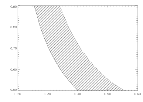
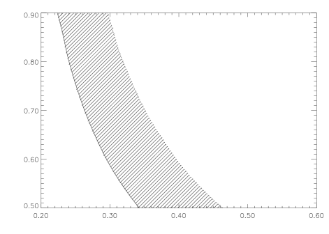
FIG. 2.: Domain wall dominated models compatible with constraints on $\sigma_{8}$ from X-ray clusters. The solid line indicates the stringent lower limit and the dotted line the upper limit, which can be weakened by including a tensor component. The vertical and horizontal axes are $h$ and $\Omega_{\rm m},$ respectively. The left and right panels indicate the spectral indices $n=1.0$ and $n=1.1$, respectively. In both cases the longitudinal sound speed is $c_{s}=0.2.$

An important test for any cosmological model is whether it can create the large-scale structure (LSS) seen today when normalized to the the CMB anisotropies observed by COBE. The simplest version of this is to compare the COBE normalized value of $\sigma_{8}$, the variance of the density field in spheres of radius $8h^{-1}{\rm Mpc},$ with that obtained from the observations of X-ray clusters [17]. Models with $w=-1$ pass this test, but two effects can cause models with $w>-1$ to predict a lower $\sigma_{8}$ when normalized to COBE: a large integrated Sachs-Wolfe component reduces the predicted value of $\sigma_{8}$, and for larger $w$ the growth of perturbations becomes stunted earlier because the SDM (or quintessence) component begins to dominate the universe earlier. To investigate the viability of these models we compute the COBE normalized $\sigma_{8}$ for $w=-2/3$ and a range of values in the $\Omega_{\rm m}-h$ plane, which are then compared to the recently computed observational value [17] $\sigma_{8}\Omega_{\rm m}^{\gamma}=(0.5-0.1\Theta)\pm 0.1$, where $\gamma=0.21-0.22w+0.33\Omega_{\rm m}+0.25\Theta$ and $\Theta=(n-1)+(h-0.65)$, valid in the range of parameters considered. Fig. 2 shows the regions of $\Omega_{\rm m}-h$ plane which pass this test for spectral indices $n=1.0$ and $n=1.1.$ For $n=1.0,$ the preferred values for quintessence models $h=0.65$ and $\Omega_{\rm m}=0.3$ are marginally incompatible with the quoted values for $\sigma_{8}$, but this situation is easily rectified by increasing $h$. Furthermore, these parameters are compatible with $n=1.1$, although the viability of scenarios with $w=-1/3$ would require even larger values of $n$. The constraint from the upper bound on $\sigma_{8}$ is weaker because of the possibility of including a tensor contribution to the CMB anisotropies [6].

We have shown that the SDM proposal, and in particular a domain wall dominated universe, is compatible with LSS via the COBE normalization/$\sigma_{8}$ test and that the inclusion of a SDM component, as opposed to quintessence, can have some potentially interesting effects on the CMB anisotropies. If the SNIa results are confirmed, an important question will be how to distinguish between SDM and quintessence models. Some possibilities include cross-correlating the CMB with LSS using, for example the X-ray background [18], or the gravitational lensing of the CMB [19]. Observations of gravitational lensing can measure the evolution of the power spectrum with redshift [20, 21], and in particular the proposed Dark Matter Telescope would measure the growth of perturbations with high accuracy.

We would like to thank Brandon Carter, Neil Turok, and Alexander Vilenkin for useful discussions, and Uros Seljak and Matias Zaldariagga for the use of CMBFAST. RAB was funded by Trinity College, MB was supported by PPARC, and DNS was supported in part by MAP.

REFERENCES

- [1] S. Perlmutter et al, Ap. J. 517, 565 (1999). A. Riess et al, A.J. 117, 207 (1998). B. Schmidt et al, Ap. J. 507, 46 (1998). P. Garnavich et al, Ap. J. 509, 74 (1998).
- [2] S.M. Carroll, W.H. Press and E.L. Turner, Ann. Rev. Astron. Astrophys. 30, 499 (1992). S. Weinberg, Rev. Mod. Phys. 61, 1 (1989).
- [3] B. Ratra and P.J.E. Peebles, Phys. Rev. D37, 3406 (1988). J. Frieman, C. Hill, A. Stebbins and I. Waga, Phys. Rev. Lett. 75, 2077 (1995). P. Viana and A. Liddle, Phys. Rev. D57, 674 (1998). K. Coble, S. Dodelson and J. Frieman, Phys. Rev. D55, 1851 (1997). R.R. Caldwell, R. Dave and P. Steinhardt, Phys. Rev. Lett. 80, 1582 (1998). M. Turner and M. White, Phys. Rev. D56, 4439 (1997). ; T. Chiba, N. Sugiyama and T. Nakamura, (1997) MNRAS 289, L5 (astro-ph/9704199); T. Chiba, N. Sugiyama and T. Nakamura (1998) MNRAS 301,72 (astro-ph/9806332)
- [4] M. Bucher and D.N. Spergel, Phys.Rev. D60 (1999) 043505 (astro-ph/9812022)
- [5] W. Hu, Ap. J. 506, 45 (1998).
- [6] R.A. Battye, M. Bucher and D.N. Spergel, In preparation.
- [7] A. Vilenkin and E.P.S. Shellard, Cosmic Strings and Other Topological Defects (Cambridge University Press, 1994).
- [8] T. Vachaspati and A. Vilenkin, Phys. Rev. D35, 1131 (1987).
- [9] V. Poenaru and G. Toulouse, J. Phys. (Paris) 38, 887 (1977). F. Bais, Nucl. Phys. B170, 32 (1980). M. Bucher, Nucl. Phys. 350, 163 (1990).
- [10] A. Vilenkin, Phys. Rev. Lett. 53, 1016 (1984).
- [11] D.N. Spergel and U.L. Pen, Ap. J. 491, L67 (1997). P. McGraw, Phys. Rev. D57, 3317 (1998).
- [12] B. Ryden, W.H. Press and D.N. Spergel, Ap. J. 357, 293 (1990).
- [13] H. Kubotani, Prog. Theor. Phys. 87, 387 (1992).
- [14] L. Wang, R.R. Caldwell, J.P. Ostriker and P.J. Steinhardt, astro-ph/9901388.
- [15] M.White, Ap. J. 506, 495 (1998).
- [16] G. Huey, L. Wang, R. Dave, R.R. Caldwell and P.J. Steinhardt, Phys. Rev. D59, 063005 (1999).
- [17] V. Eke, S. Cole and C. Frenk, MNRAS 282, 263 (1996). L. Wang and P.J. Steinhardt, Ap. J. 508, 483 (1998).
- [18] R. Crittenden and N. Turok, Phys. Rev. Lett. 76, 575 (1996).
- [19] R.B. Metcalf and J. Silk, astro-ph/9708059.
- [20] W. Hu, astro-ph/9904153.
- [21] http://www.dmtelescope.org/