$UBVI$ Color-Magnitude Diagrams in Baade’s Window: Metallicity Range, Implications for the Red Clump Method, Color “Anomaly” and the Distances to the Galactic Center and the Large Magellanic Cloud

Abstract

We analyze the $UBVI$ color-magnitude diagrams towards the Galactic bulge in a relatively low-reddening region of Baade’s Window. The dereddened red giant branch is very wide [$\sim 1.0\;$mag in $(U-B)_{0}$ and $\sim 0.4\;$mag in $(B-V)_{0}$ and $(V-I)_{0}$], indicating a significant dispersion of stellar metallicities, which by comparison with the theoretical isochrones and data for Galactic clusters we estimate to lie between approximately $-0.7<[Fe/H]<+0.3$, i.e. spanning about $1\;dex$ in metallicity, in good agreement with earlier spectroscopic studies.

We also discuss the metallicity dependence of the red clump $I$-band brightness and we show that it is between $0.1-0.2\;mag\;dex^{-1}$. This agrees well with the previous empirical determinations and the models of stellar evolution.

The de-reddened $(V-I)_{0}$ color of the red clump in the observed bulge field is $\langle(V-I)_{0}\rangle=1.066$, $\sigma_{(V-I)_{0}}=0.14$, i.e. $0.056\;$mag redder than the local stars with good parallaxes measured by Hipparcos. It seems that the large “color anomaly” of $\sim 0.2\;$mag noticed by Paczyński & Stanek and discussed in many recent papers was mostly due to earlier problems with photometric calibration. When we use our data to re-derive the red clump distance to the Galactic center, we obtain the Galactocentric distance modulus $\mu_{0,GC}=14.69\pm 0.1\;$mag ($R_{0}=8.67\pm 0.4\;kpc$), with error dominated by the systematics of photometric calibration.

We then discuss the systematics of the red clump method and how they affect the red clump distance to the Large Magellanic Cloud. We argue that the value of distance modulus $\mu_{0,LMC}=18.24\pm 0.08$ $(44.5\pm 1.7\;kpc)$, recently refined by Udalski, is currently the most secure and robust of all LMC distance estimates. This has the effect of increasing any LMC-tied Hubble constant by about 12%, including the recent determinations by the HST Key Project and Sandage et al.

The $UBVI$ photometry is available through the anonymous ftp service.

1 INTRODUCTION

The intermediate-age, degenerate core helium-burning stars, known as the “red clump” stars, form a very pronounced and compact structure on the color-magnitude diagrams (CMDs) in variety of stellar populations. Indeed the absolute magnitude-color diagram of the Solar neighborhood obtained by Hipparcos (Perryman et al. 1997) clearly shows how compact the red clump is. Therefore, it could be expected that this equivalent of the better known horizontal branch stars in old, metal poor stellar populations, would be potentially a very good standard candle. However, in spite of their large number and good theoretical understanding these stars have seldom been used as the distance indicators. Stanek (1995) and Stanek et al. (1994, 1997) used these stars to map the Galactic bar. Considering that the red clump is the only distance indicator well calibrated with the Hipparcos trigonometric parallaxes (with $\sim 10^{3}$ red clump stars with parallaxes better than 10%), it becomes very important to understand various possible systematics of this method.

As noticed by Paczyński & Stanek (1998), the peak $I$-band brightness of the red clump is remarkably constant over a broad range of $V-I$ colors. This lack of correlation of red clump $I$-band brightness with $V-I$ color was further confirmed by data from such varied populations as the halo and globular clusters in M31 (Stanek & Garnavich 1998), field stars in the LMC (Udalski et al. 1998; Stanek, Zaritsky & Harris 1998) and the SMC (Udalski et al. 1998) and clusters in the LMC and the SMC (Udalski 1998b). This was interpreted as lack of strong dependence of the red clump $I$-band brightness on the metallicity, a very desirable feature for any distance indicator. This conclusion was however questioned, among others by Girardi et al. (1998). They made use of a large set of evolutionary tracks to show that more massive clump models are systematically bluer than the less massive ones. They argue that the color range spanned by the red clump stars is largely caused by the dispersion of masses (and hence ages), and not their metallicity. It is therefore important to be able to distinguish between these two possibilities, which we attempt in this paper using multiband $UBVI$ data for a stellar field in a low reddening region of Baade’s Window. As we show in this paper, the large range in color of the bulge red clump stars is mostly due to large metallicity range of these stars. We use this fact to put limits on the metallicity dependence of the red clump $I$-band luminosity.

We describe the data and the deredenning procedure in Section 2. In Section 3 we compare the bulge data with the multiband observations of Galactic clusters and with the theoretical isochrones, and we estimate the metallicity range for the bulge. In Section 4 we discuss the metallicity dependence of the red clump. In Section 5 we discuss the “color anomaly” of the bulge red clump and derive the red clump distance to the Galactic center. Finally, in Section 6 we discuss the possible systematics of the red clump distance determination method and argue it provides currently the most robust distance to the LMC.

2 THE DATA AND THE DEREDDENING PROCEDURE

The data were obtained with the Las Campanas Observatory 2.5-meter DuPont telescope using a thinned Tektronix CCD – known as TEK5 camera – with the pixel scale of $0.262\;arcsec\;pixel^{-1}$ and the field of view $8.9\arcmin\times 8.9\arcmin$. We observed a low-reddening part of Baade’s Window (Figure 1), falling within OGLE field BW8 (Udalski et al. 1993).

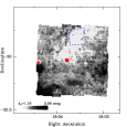
Figure 1: $A_{V}$ extinction map of Baade’s Window (Stanek 1996), along with the BW8 field analyzed in this paper (dashed square). The two black dots correspond to the globular clusters NGC6522 (center) and NGC6528 (left).

Most of the data were obtained on the night of April 22/23, 1995 (UT). A list of frames collected on that night and used to extract photometry presented in this paper is given in Table 1. Only $UBV$ filters were used during the April run. However, the night of April 22/23, 1995 turned out to be non-photometric, therefore on the night of July 20/21, 1995 we collected single $UBVI$ frames (V-60 sec, B-60 sec, U-180 sec, I-40 sec) of the field offset $3.75\arcmin$ east relatively to the field observed in April. The same equipment was used during both runs, with the exception of the B filter. The following relations were derived, by comparison with the Landolt (1992) standard stars, to transform July photometry to the standard $UBVI_{C}$ system:

$$v=b_{1}+V-0.016\times(B-V)+0.144\times X$$ (1)

$$i=b_{2}+I-0.042\times(V-I)+0.05\times X$$ (2)

$$b-v=b_{3}+0.867\times(B-V)+0.128\times X$$ (3)

$$u-b=b_{4}+0.956\times(U-B)+0.176\times X$$ (4)

$$v-i=b_{5}+1.057\times(V-I)+0.08\times X$$ (5)

Figure 2: $I$-band brightness vs. $(U-B),(B-V)$ and $(V-I)$. Note that the lack of red clump stars with $(U-B)>1.9$ is real and is not a detection artifact.

Table 1: Observing log

	$T_{exp}$	FWHM
Filter	[$sec$]	[$arcsec$]
$V$	$3\times 200$	1.00
$V$	$3\times 200$	0.97
$V$	$1\times 40$	0.79
$B$	$2\times 500$	1.10
$B$	$3\times 500$	0.86
$B$	$3\times 500$	0.89
$B$	$1\times 60$	0.89
$U$	$3\times 900$	1.00

The $UBVI$ photometry obtained in July was used to establish zero points of the $UBV$ data collected during the April run. The instrumental photometry was extracted using Daophot/Allstar package (Stetson 1987). In case of the profile photometry we used gaussian type empirical PSF varying quadratically with $X,Y$ coordinates. Measurements with relatively large errors (for given magnitude) or exceptionally large values of Daophot parameters CHI1,CHI2 were flagged and not used for the analysis. The fraction of measurements rejected for a given frame ranged from a few percent up to 65%. That means that we sacrificed completeness of the photometry for the sake of its internal accuracy.

We also derived equatorial coordinates for all stars, using the USNO-A2.0 catalog (Monet et al. 1996), with an average difference of $0.7\arcsec$ for the 215 transformation stars found in both catalogs. The field center is at $[(\alpha,\delta)=(18\!\!:\!\!03\!\!:\!\!08.1,-29\!\!:\!\!48\!\!:\!\!44),{\rm J2000.0}]$. The $UBVI$ data and the coordinates of the stars can be accessed from anonymous ftp at ftp://cfa-ftp.harvard.edu/pub/kstanek/BW8/.

In Figure 2 we plot the $I$-band brightness, for the stars in the field BW8, versus all three independent colors $(U-B),(B-V)$ and $(V-I)$. The non-standard choice of plotting the $I$-band brightness versus color is to show that the red clump $I$-band brightness is basically independent of color. For more detailed discussion of main features in the CMDs toward the Galactic bulge see Kiraga, Paczyński & Stanek (1997). The most striking feature of the current CMDs (Figure 2) is the increasing width, in color, of both the red clump and also the red giant branch, as we move from the $(V-I)$ color to the $(U-B)$ color. The red clump and the red giants branch become so wide in the $(U-B)$ color that they overlap with the foreground Galactic disk stars.

We also use the data for two Galactic clusters for comparison purposes. The $BVI$ CMDs of the Galactic globular cluster 47Tuc were taken from Kaluzny et al. (1998). The $UBVI$ data for an old open cluster NGC6791 were taken from Kaluzny & Udalski (1992) and from Kaluzny & Rucinski (1995).

By design, we observed a relatively uniform- and low-reddening part of Baade’s Window, in order to minimize the effects of reddening in our CMD studies. To deredden the CMDs in the BW8 field, we used the $A_{V},E(V-I)$ extinction map of Baade’s Window by Stanek (1996), based on the method of Woźniak & Stanek (1996) and the OGLE data of Udalski et al. (1993). The zero point for Stanek (1996) map was determined by Gould, Popowski & Terndrup (1998) and Alcock et al. (1998). Figure 3 shows the distribution of the $E(V-I)$ reddening for stars located in the BW8 field, derived using map of Stanek (1996). The $E(V-I)$ reddening is quite uniform across the field, with small $rms$ scatter of $\sigma_{E(V-I)}=0.05\;$mag. To remove the effects of extinction in the $UB$ bands we used the standard coefficients, as given for example by Schlegel, Finkbeiner & Davis (1998, hereafter: SFD), $A_{B}/A_{V}=1.324$ and $A_{U}/A_{V}=1.521$.

Figure 3: Distribution of the $E(V-I)$ reddening for stars located in the BW8 field, derived using the map of Stanek (1996). The reddening is fairly uniform across the field, with $rms$ scatter of $\sigma_{E(V-I)}=0.05\;$mag.

For the two clusters we have taken the reddening values from the SFD map, $E(B-V)_{47Tuc}=0.031$ and $E(B-V)_{NGC6791}=0.15$. In both cases the SFD reddening values are very uniform over the clusters. In case of 47Tuc the cluster is located at high galactic latitude of $b=-44\arcdeg\!.9$, so the SFD value of reddening very likely represents the total, low, reddening towards the cluster. In case of NGC6791, located at low galactic latitude of $b=10\arcdeg\!.9$, it is possible that some of the reddening measured by the SFD map could be located behind the cluster. Indeed, in a recent detailed study of this cluster by Chaboyer, Green & Liebert (1999) they obtain the best-fit value of $E(B-V)=0.10$, with the acceptable range of $0.08\leq E(B-V)\leq 0.13$. On the other hand, NGC6791 is located at approximately $4.2\;kpc$ from the Sun, which gives a distance from the Galactic plane of about $800\;pc$, i.e. most probably well outside the Galactic plane dust layer. We therefore assume for this cluster the SFD value of $E(B-V)_{NGC6791}=0.15$, which has the advantage of being independent from the color-magnitude data itself, and in fact is close to some of the previous determinations [e.g. $E(B-V)=0.17$, Kaluzny & Rucinski 1995]. In any case, small changes in this value only weakly affect any results of comparison with the Galactic bulge data discussed in the next Section.

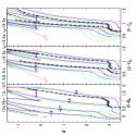
Figure 4: Theoretical isochrones from Bertelli et al. (1994), for four metallicities: $[Fe/H]=-1.3,-0.7,0.0$ and $+0.4$. For each metallicity the isochrones corresponding to ages of 5.0, 10.0 and $15.0\;Gyr$ are plotted ($5.0\;Gyr$: dashed lines; $10.0\;Gyr$: continuous; $15.0\;Gyr$: dotted). Also shown are the dereddened CMDs for 47Tuc ($[Fe/H]\approx-0.7$: triangles) and NGC6791 ($[Fe/H]\approx+0.3$: circles). The red clump is represented by the kink at $M_{I}\approx-0.2$ in the model isochrones.

3 METALLICITY RANGE IN THE GALACTIC BULGE

There have been several papers investigating spectroscopically the abundance properties of the Galactic bulge, such as Rich (1988), McWilliam & Rich (1994), Minniti et al. (1995) and Sadler, Rich & Terndrup (1996). They studied chemistry of giants in the Galactic bulge, Rich (1998), McWilliam & Rich (1994) and Sadler et al. (1996) in Baade’s Window and Minniti et al. (1995) in several other bulge fields. From all these papers it is clear that while the mean metallicity of the bulge is close to the solar value, at any given field there is a large spread in metal abundances, possibly as large as $2\;dex$ (see Figures 17 and 19 of McWilliam & Rich, Figures 3-5 of Minniti et al. and Figure 11 of Sadler et al.). In this paper we want to put additional constraints on the metallicity distributions, using the multiband $UBVI$ photometric data. The spectroscopy is much superior to photometry when it comes to metallicity investigations for limited number of stars, but the photometry has the advantage of providing some metallicity information for much larger samples of stars.

We start by investigating the behavior of theoretical models of stellar evolution, calculated by Bertelli et al. (1994). We select four metallicities, corresponding to $[Fe/H]=-1.3,-0.7,0.0$ and $+0.4$. To illustrate the effect of age on the predicted colors and luminosities, for each metallicity we take three isochrones, corresponding to ages of 5.0, 10.0 and $15.0\;Gyr$, as to bracket the most likely age for the population of the Galactic bulge (e.g. Sevenster 1999). In Figure 4 we plot the model isochrones, showing $M_{I}$ luminosity as a function of $(U-B)_{0},(B-V)_{0},(V-I)_{0}$ for each metallicity and age.

Also in Figure 4 we plot the dereddened CMDs (plotted as maximum density ridge-lines only) for 47Tuc and NGC6791. In the recent compilation Harris (1996) lists for 47Tuc a metallicity of about $[Fe/H]\approx-0.7$. Kaluzny et al. (1998) has determined its distance modulus to be $(m-M)_{0,47Tuc}=13.32\;$mag. For NGC6791 Chaboyer et al. (1999) have derived a metallicity of $[Fe/H]=+0.4$, somewhat higher than Kaluzny & Rucinski (1995: $[Fe/H]=+0.3$) and Garnavich et al. (1994: $[Fe/H]=+0.2$), and distance modulus of $(m-M)_{0,NGC6791}=13.11\;$mag. We adopt $[Fe/H]=+0.3$ for this cluster. As we are going to use both these clusters only through their RGBs, as a fiducial points for the metallicity determination, the exact values of their distance moduli are not very important, since the RGBs of the clusters are fairly vertical. The adopted reddenings are more important, but the differences are not significant from the point of view of this paper.

As discussed by Girardi et al. (1998), when modelling the Hipparcos CMD for the Solar neighborhood, the colors of the Bertelli et al. (1994) isochrones are systematically shifted to the redder color. Indeed, to make the Bertelli et al. (1994) isochrones agree with the colors of the two clusters, we had to subtract $0.10\;$mag from the theoretical $(B-V)$ color and $0.08\;$mag from the $(V-I)$ color.

Figure 5: $M_{I}$ absolute magnitude - dereddened color diagrams for the BW8 field. Also plotted are the $t=10\;Gy$ isochrones and the the dereddened maximum density ridge-lines for 47Tuc ($[Fe/H]\approx-0.7$: triangles) and NGC6791 ($[Fe/H]\approx+0.3$: circles).

There is a number of interesting features in Figure 4. For example, the oldest and lowest metallicity isochrone ($[Fe/H]=-1.3,t=15\;Gy$) does not have a red clump, but has a clear horizontal branch. However, all the remaining isochrones have well defined red clump, with its $(U-B)_{0}$ and $(B-V)_{0}$ colors quite strongly dependent on the metallicity, but only weakly dependent on age. However, it is worth noticing that the $(V-I)_{0}$ color of the red clump is basically the same for low metallicities, $(V-I)_{0}\approx 0.8$, both from observations (Udalski et al. 1998) and from the theoretical isochrones. The $I$-band brightness of the red clump, as given by the isochrones, varies only little with age and metallicity. For each age, higher metallicity corresponds to redder RGB (clearly seen between $2.0<M_{I}<0.0$), while for each metallicity older age also corresponds to redder RGB. The model dependence of the RGB color on age is also much weaker than the metallicity dependence, especially in the $(U-B)_{0}$ color.

As the next step, using the RGB we want to constrain the metallicity distribution for stars in our BW8 Galactic bulge sample. As discussed above, the age effect on color is small, so for each metallicity we will use the $t=10\;Gy$ isochrone as the representative one. In Figure 5 we plot the BW8 CMDs along with the theoretical isochrones and the clusters data. The BW8 data has been dereddened using the prescription described in the previous section, and also shifted by distance modulus of $\mu_{0,GC}=14.57\;$mag determined by Stanek & Garnavich (1998).

As mentioned before, the RGB stars from the Galactic bulge overlap in the $(U-B)$ color with the foreground Galactic disk main sequence stars, and the full width of the red bulge giant branch is about $\sim 1.0\;$mag in this color. However, the RGB can be seen as a separate feature when measured in $(B-V)$ and $(V-I)$ colors, with a full width of about $\sim 0.4\;$mag. We will not attempt to derive a detailed distribution in metallicity of the bulge RGB stars, as the current sample of stars is not very large, and the colors of theoretical isochrones are subject to problems discussed earlier in this Section. Nevertheless, it is readily apparent that the metallicity range of the bulge RGB stars extends approximately from that of 47Tuc ($[Fe/H]=-0.7$) to that of NGC6791 ($[Fe/H]=+0.3$), i.e. at least $1\;dex$ in metallicity, with average metallicity close to the Solar value. This agrees well with the spectroscopic determinations discussed above (Rich 1988; McWilliam & Rich 1994; Minniti et al. 1995; Sadler, Rich & Terndrup 1996).

It should be stressed here that the comparison of data with the theoretical isochrones and CMDs of clusters serves only to establish a rough metallicity range of the bulge stars. As discussed in Paczyński et al. (1999), an observational program to establish how good the correlation is between the metallicity and the colors would be most useful. Such correlations for the local stars can be seen in the first astro-ph version of Udalski (2000).

4 METALLICITY DEPENDENCE OF THE RED CLUMP

As discussed by Paczyński (1998) and Udalski (2000), the subject of the metallicity dependence of the red clump brightness has important consequences for the applicability of the method for the distance measurements. Paczyński & Stanek (1998) have found that the brightness of the red clump in the $I$-band does not depend on the $(V-I)_{0}$ color over a broad range, which they expected to correlate well with the metallicity. However, Paczyński (1998) has found no such correlation between the $[Fe/H]$, obtained using Washington CCD photometry (Geisler & Friel 1992), and the color of the red clump giants in the Galactic bulge.

Another approach to the question of the red clump metallicity dependence comes from the population synthesis models. Cole (1998), in a very preliminary attempt, has derived a value for the metallicity dependence of $0.21\pm 0.07\;mag\;dex^{-1}$, using models of Seidel, Demarque & Weinberg (1987), which by 1998 were already considered obsolete (see discussion in Gibson 2000). More sophisticated and modern calculations of Girardi et al. (1998) and Girardi (1999) give a somewhat smaller value of $\sim 0.15\;mag\;dex^{-1}$ (this value, not given explicitly by the author, was obtained from plots in Figures 4 and 7 of Girardi 1999). This should be compared to two empirical determinations: $0.09\pm 0.03\;mag\;dex^{-1}$ by Udalski (1998a) and more recent one of $0.13\pm 0.07\;mag\;dex^{-1}$ by Udalski (2000). Popowski (2000) has re-analyzed the data of Udalski (1998a) and has derived the red clump metallicity dependence of $0.19\pm 0.05\;mag\;dex^{-1}$. And while more work needs to be done on this problem, it is already clear that the metallicity dependence of the red clump brightness is modest ($0.1-0.2\;mag\;dex^{-1}$) and that theory and observations are in a good agreement on the subject.

It is well worth noticing here that the data of Udalski (1998b) for star clusters in the LMC and the SMC, used originally to show a weak dependence of the red clump brightness on age, also provide reasonable constrains on the red clump metallicity dependence. For example, the SMC cluster L11 with $[Fe/H]=-0.70$ and age of $3.5\;Gyr$, has the dereddened peak magnitude of the red clump only $0.03\;mag$ different from another SMC cluster, NGC339, which has $[Fe/H]=-1.4$ and age of $4.0\;Gyr$ (Da Costa & Hatzidimitriou 1998). Even with relatively low metallicity, NGC339 has a well-developed red clump, which agrees with theoretical expectations (Figure 4).

Additional constraint for the red clump metallicity dependence comes from the data analyzed in this paper. As we have shown in the previous section, the bulge RGB spans about $1\;dex$ in metallicity, from which follows naturally that the bulge red clump stars also have a large metallicity range. At the same time, as noticed by Paczyński & Stanek (1998), the peak $I$-band brightness of the red clump is remarkably constant over a broad range of $(V-I)_{0}$ colors. In the previous section we have shown that the model isochrones suggest a good correlation between the metallicity and the color, and the data presented in this paper support that strongly. Paczyński & Stanek (1998) have found a $0.09\;$mag difference in brightness between the red clump stars with $1.0<(V-I)_{0}<1.1$ and those with $1.3<(V-I)_{0}<1.4$ (their Fig. 1), with the redder stars fainter than the bluer stars. Their red clump stars with $0.8<(V-I)_{0}<1.0$ were however again fainter than those with $1.0<(V-I)_{0}<1.1$, but the bulge red clump was not very well defined in this color range. If we take this to represent the difference in brightness of red clump stars with different metallicity, this gives us a small metallicity dependence of $\sim 0.1\;mag\;dex^{-1}$, using the Galactic bulge metallicity range derived in the previous section. This is in good agreement with the empirical determination of $0.13\pm 0.07\;mag\;dex^{-1}$ obtained by Udalski (2000), and also in good agreement with the theoretical expectations.

Paczyński et al. (1999) have presented $UBVI$ photometry in a nearby field BWC in Baade’s Window. Their results are overall in a substantial agreement with ours, although there are some systematic differences in the photometric zero points on the order of a few hundredths of magnitude. These have no overall significance for the main conclusions presented in this paper and in the paper of Paczyński et al. (1999). One aspect which is affected, the “color anomaly” of the red clump, is discussed in the next section.

5 “COLOR ANOMALY” OF THE RED CLUMP AND THE DISTANCE TO THE GALACTIC CENTER

As first noticed by Paczyński & Stanek (1998), the dereddened red clump observed by OGLE-I in Baade’s Window was $\sim 0.2\;$mag redder than in the Solar neighborhood. Were this “color anomaly” real, it would have important consequences, as extensively discussed by Paczyński (1998), Paczyński et al. (1999), Popowski (2000), Alves (2000) and Gould, Stutz & Frogel (2000).

We have therefore decided to repeat the procedure of Paczyński & Stanek (1998) and derive the dereddened $(V-I)_{0}$ color of the red clump in the bulge. The results can be seen in Figure 6, analogous to Figure 4 of Paczyński & Stanek (1998). The de-reddened $(V-I)_{0}$ color of the red clump in the Galactic bulge is $\langle(V-I)_{0}\rangle=1.066$, $\sigma_{(V-I)_{0}}=0.14$, i.e. $0.056\;$mag redder than the local stars with good parallaxes measured by Hipparcos. However, huge “color anomaly” of $\sim 0.2\;$mag seen by Paczyński & Stanek (1998) is mostly eliminated. The remaining difference of $0.056\;$mag could be real: the chemical composition of the bulge stars is somewhat different from the local stars, although there is substantial overlap (see Figure 1 of Udalski 2000). Given that the main difference between the analysis of Paczyński & Stanek (1998) and the current paper is in the different photometric data used, we suspect that most of the “color anomaly” resulted from CCD non-linearity of OGLE-I data (Kiraga et al. 1997) and resulting problems with photometric calibration. The fact that the new OGLE-II data give $(V-I)_{0}=1.11$ (Paczyński et al. 1999), i.e. $\sim 0.1\;$mag smaller “color anomaly”, support this conclusion (see discussion in Popowski 2000).

Figure 6: The number of red clump stars in the solar neighborhood, based on Hipparcos data, is shown as a function of their $(V-I)$ color with the thin solid line. The number of red clump stars in the BW8 field is shown as a function of their $(V-I)_{0}$ color with the thick solid line. All distributions are normalized, and include all stars with their absolute magnitude within $0.3\;$mag of $M_{I,m}$.

Given a likely problem with the OGLE-I photometric data, which were used by Paczyński & Stanek (1998), we decided to re-derive the red clump distance to the Galactic center with current data. We have followed exactly the procedure of Paczyński & Stanek (1998): we selected the red clump stars in the color range $0.8<(V-I)_{0}<1.25$ in the BW8 field and we fitted the resulting distribution with their Eq.1. The fitted Gaussian peak of the red clump distribution was at $I_{0,m}=14.447\pm 0.02$ (statistical error only), $0.12\;$mag fainter than that of Paczyński & Stanek. This, combined with corrections due to the geometry of the Galactic bar (Stanek et al. 1997) and revised $I$-band calibration of the local red clump (Stanek & Garnavich 1998), gives the Galactocentric distance modulus $\mu_{0,GC}=14.69\pm 0.1\;$mag, with corresponding Galactocentric distance $R_{0}=8.67\pm 0.4\;kpc$. We set the error to fairly conservative $0.1\;$mag to allow for possible errors in photometric calibration of current data.

This value can be compared to two recent determinations. The first one, by Alves (2000), uses the infrared $K$-band version of the red clump method, and is therefore much less susceptible to errors in the reddening correction. His value is $R_{0}=8.24\pm 0.42\;kpc$, with the error dominated by small number of bulge red clump giants with good $K$-band photometry. Another determination comes from Gould et al. (2000), who obtained $R_{0}=8.63\pm 0.16\;kpc$ (statistical error only). This was obtained by using the value for the $I$-band peak of the red clump from Paczyński et al. (1999), but after it was adjusted for, different from Stanek (1996), value of the ratio of total to selective extinction $R_{VI}$ (see Gould et al. 2000 for discussion). Note that the value of Gould et al. is extremely close to that obtained in this Section, but even the lower value of Alves (2000) is in good statistical agreement and within 5% of our value.

Figure 7: The color – color diagram: $(B-V)_{0}-(U-B)_{0}$ for red clump giants in the BW8 field, corrected for interstellar reddening. The two thin lines that cross are the regression lines of one color with respect to another, derived by Paczyński et al. (1999) from the local stars with Hipparcos parallaxes better than 10%.

Figure 8: The color – color diagram: $(V-I)_{0}-(B-V)_{0}$ for red clump giants in the BW8 field, corrected for interstellar reddening. The two thin lines that cross are the regression lines of one color with respect to another, derived by Paczyński et al. (1999) from the local stars with Hipparcos parallaxes better than 10%.

To further explore the issues related to photometric calibration, following Paczyński et al. (1999) we decided to investigate the color-color properties of our sample of red clump giants. This was done exactly as in Paczyński et al. (1999) paper, and the results are presented in Figures 8 and 8, analogous to Figures 6 and 7 in their paper. The sequences defined by the bulge giants are fairly close to those defined by the local stars, although there seems to be a small systematic offset, possibly due to small errors in the photometric calibration.

It is clear from the above discussion that the issue of accurate photometric calibration is of crucial importance in these extremely crowded Galactic bulge fields. In addition, due to fairly large reddening, the exact properties of interstellar extinction need to be better understood (see Gould et al. 2000 for discussion of one of the possible problems).

6 RED CLUMP SYSTEMATICS AND THE DISTANCE TO THE LMC

The distance to the LMC is one of the most important problems of the modern astrophysics, because the extragalactic Cepheid-based distance scale is tied to it (e.g. Mould et al. 2000). Most reviews of the subject place the LMC at the distance modulus of $\sim 18.5\pm 0.1\;$mag, but values as high as $\sim 18.7$ are also present in the literature (Feast 1999). The errors in this distance are quoted sometimes as being as small as $0.05\;$mag (e.g. van den Bergh 2000, Carretta et al. 2000), although these small error bars are obtained by statistically unjustified procedures of ignoring strong outliers or assigning them arbitrarily large error bars. It should be noted that averaging various distance estimates while they are dominated by their systematic errors is a risky statistical proposition. For a good discussion of the distance to the LMC derived from different methods see Jha et al. (1999) and Gibson (2000).

As discussed throughout this paper, the systematics of the red clump method seem to be quite well understood, both empirically and theoretically. In the rest of this Section we will present a summary of various factors affecting the robustness of the red clump distance to the LMC and compare it with other commonly used methods.

Zero point calibration

As for any other distance indicator, it is important to know the brightness of the red clump for some selected stellar population. This was provided by the Hipparcos satellite, which measured $\sim 10^{3}$ red clump stars with better than 10% parallaxes (Perryman et al. 1997). Stanek & Garnavich (1998) selected from them a sub-sample of 228 red clump stars with the distance $d<70\;pc$. They found that the red clump $I$-band absolute magnitude $M_{I,m}(d<70\;pc)=-0.227\pm 0.023$ for these nearby stars, with the average distance $\langle d_{<70}\rangle=50\;pc$. One expects very little reddening, $E(B-V)<0.02$, for such nearby stars, so they assumed that their $d<70\;pc$ sample suffered no reddening. As follows from detailed discussion of the local interstellar medium by Ferlet (1999), this assumption is unlikely to produce any significant ($>0.05\;mag$) error — we live in the Local Bubble, largely devoid of stellar extinction. This assumption can be further tested by comparing the brightness of various spatial sub-samples of the red clump, e.g. low-$b$ vs. high-$b$ samples.

It is worth mentioning that Girardi et al. (1998) have applied the Lutz-Kelker (1973) bias correction while calculating the value of $M_{I,m}$ for the Hipparcos red clump and have obtained a value of $M_{I,m}=-0.21$, i.e. practically identical to that of Stanek & Garnavich (1998).

It should be stressed that Hipparcos provided accurate distance determinations for over 1,000 red clump stars, but unfortunately $I$-band photometry is available for only $\sim 50\%$ of them, so it would be important to obtain $I$-band photometry for all Hipparcos red clump giants. This would further reduce the already very small statistical zero-point error and would allow better testing of any systematic errors.

It is beyond the scope of this paper to provide detailed reviews of the zero-point calibrations for the other commonly used distance indicators, so the interested reader should consult Popowski & Gould (1999) for the RR Lyrae stars, Carretta et al. (2000) for the subdwarf fitting technique and Feast (1999) for the Cepheids zero point (or one of several other reviews).

To provide some comparison with the red clump Hipparcos zero point calibration, based on many hundreds of stars measured with better than 10% parallaxes, there is only one RR Lyrae with reasonable trigonometric parallax (RR Lyrae itself: Popowski & Gould 1999), similarly for the Cepheid variables (Polaris: Feast & Catchpole 1997). There is somewhat more Hipparcos-measured subdwarfs, from about 15 in Reid (1997) to about 30 in Carretta et al. (2000). It is fair to say that the red clump stars are the only well represented distance indicator in the sample of Solar neighborhood stars with trigonometric parallaxes well measured by Hipparcos.

Metallicity dependence

Again, as with any distance indicator, also red clump stars are subject to possible metallicity dependence. We have reviewed this problem throughout this paper, so let us stress again that this dependence for the red clump is modest ($\sim 0.1-0.2\;mag\;dex^{-1}$) and the empirical determinations agree well with the model calculations. This is quite unlike the Cepheids, where the empirical determinations range from 0 to $-0.4\;mag\;dex^{-1}$ (Freedman & Madore 1990; Sasselov et al. 1997; Kochanek et al. 1997; Kennicutt et al. 1998), while the theoretical determinations often have even different sign of the metallicity effect (e.g. Gautschy 1998). The situation for the metallicity dependence of RR Lyrae stars seems to be not so controversial, and the interested reader should consult any of the many recent papers on the subject (e.g. Popowski & Gould 1999). However, the metallicity is of basic importance for the subdwarf fitting method, where the metallicity of faint, locally observed subdwarfs is compared to metallicity of giants in distant globular clusters (for discussion see Popowski & Gould 1999). So, it is again fair to say that if the red clump method has any problems with the metallicity dependence, for other local Group distance indicators these problems are similar or in some cases much more severe.

Age dependence

It is possible that red clump stars would suffer from a strong age dependence. This possibility was however not confirmed by empirical determination of Udalski (1998b), who observed star clusters with different ages in the LMC and the SMC and found basically no age dependence between 2 and $10\;Gyr$. Also, modern theoretical models of Girardi et al. (1998) and Girardi (1999) do not support strong age dependence.

Recently, Sarajedini (1999) found that the $M_{I}$ peak brightness of the red clump in Galactic open clusters becomes fainter for clusters older than $5\;Gyr$. However, there are only three such clusters in his sample, so much more observational work needs to be done to firmly establish age dependence, if any. More importantly, the absolute peak brightness $M_{I}$ for each cluster is derived by Sarajedini (1999) using main sequence fitting technique, which is not without its own problems (e.g. Pinsonneault, Terndrup & Yuan 2000). Finally, even the cluster with the brightest red clump in Sarajedini’s sample, NGC 2204, has $M_{I}=-0.34$ (at $[Fe/H]=-0.34$), i.e. only $0.11\;$mag brighter than the local Hipparcos red clump (Stanek & Garnavich 1998), which gives an approximate size of population correction to the red clump LMC distance. Obviously, population effects do exist for the red clump method, but they are fairly small.

Possibly the strongest argument against significant age dependence of the red clump method, when applied to mixed populations of stars, comes from Girardi (2000). He noticed that for constant star formation rate the age distribution of clump stars is strongly biased towards intermediate ages, $1-3\;Gyr$ (his Fig. 2). This very strongly suggest that when deriving the red clump distance to objects like the LMC one largely bypasses the age problem because the majority of the red clump stars in both the local and the LMC populations are of similar age. This conclusion is also supported by the very compact red clump in the SMC, as presented by Paczyński et al. (1999, their Figure 10).

Reddening

Every method of distance determination utilizing standard candles is affected to some extent by how well the reddening and extinction along the line of sight are known. In this aspect red clump is not worse than any other method, and since it relies on the $I$-band brightness, it might be somewhat less susceptible to reddening than some other methods. In many cases where the red clump was used to derive the distance to the LMC (Udalski et al. 1998; Stanek et al. 1998; Udalski 1998a,b), particular attention was paid to come up with as accurate estimate of the reddening as possible. For example, in the paper of Stanek et al. (1998) the reddening values obtained using the reddening map of Harris, Zaritsky & Thompson (1997) were compared to those from the SFD map and in the two regions selected for further analysis the two maps agreed to within $0.02\;$mag in $E(B-V)$, or $0.04\;$mag in $A_{I}$.

Still better approach to the problem of reddening is to apply any distance determination method in regions with small reddening, if possible. Udalski (2000) used nine stellar fields in the LMC to derive the distance modulus of $18.24\pm 0.08$. The SFD map was used to obtain the reddenings, and some of the LMC fields used in his paper have reddening values as small as $E(B-V)\approx 0.03$ (see Table 1 of Udalski 2000). The approach of bypassing the reddening problem by using low extinction regions is, by design, much more preferred over complicated dust corrections applied in dusty regions (Zaritsky 1999; Romaniello et al. 2000; Sakai, Zaritsky & Kennicutt 2000). Another approach, which would eliminate most of the problems due to the reddening, would be to apply the $K$-band version of the red clump method (Alves 2000) to obtain the LMC distance.

To summarize, the major strength of the red clump distance determination technique lies in its accurate absolute magnitude as determined in the Solar neighborhood using Hipparcos data (Paczyński & Stanek 1998; Stanek & Garnavich 1998). It was also shown the the $I$-band brightness of the red clump remains remarkably constant in such varied environments as the halo and globular clusters of M31 (Stanek & Garnavich 1998), field stars in the LMC and the SMC (Udalski et al. 1998; Stanek et al. 1998) and clusters in the LMC and the SMC (Udalski 1998b). Also, as shown by Paczyński & Stanek (1998), the $I$-band brightness of the Galactic bulge red clump varies only by few hundreds of magnitude over $\sim 0.4\;$mag in $(V-I)_{0}$. This and analysis of Udalski (1998a) and Udalski (2000) indicate that there is only a modest metallicity dependence of the red clump $I$-band brightness, in agreement with the theoretical models (Girardi 1999). Also, there is no significant age dependence over a broad range of ages (Udalski 1998b). All this combined makes the distance modulus to LMC of $18.24\pm 0.08$, as determined by Udalski (2000), currently the most secure and robust of all LMC distance estimates, which has the effect of increasing any LMC-tied Hubble constant determinations by about 12%, including the recent determinations by the HST Key Project (e.g. Mould et al. 2000) and by Sandage & Tammann (1998).

NOTE TO AVOID CONFUSION:

After the first version of this paper was submitted for publication in AJ (August 1999: astro-ph/9908041), there appeared several papers discussing the properties of red clump. Some of these papers cite this paper, but are also cited in this current revised version.

References

- (1)
- (2) Alcock, C., et al. 1998, ApJ, 494, 396
- (3)
- (4) Alves, D. R. 2000, ApJ, in press (astro-ph/0003329)
- (5)
- (6) Bertelli, G., Bressan, A., Chiosi, C., Fagotto, F., & Nasi, E. 1994, A&AS, 106, 275
- (7)
- (8) Carretta, E., Gratton, R. G., Clementini, G., & Fusi Pecci, F. 2000, ApJ, 533, 215
- (9)
- (10) Chaboyer, B., Green, E. M., & Liebert, J. 1999, AJ, 117, 136
- (11)
- (12) Cole, A. A. 1998, ApJ, 500, L137
- (13)
- (14) Da Costa, G. S., & Hatzidimitriou, D. 1998, AJ, 115, 1934
- (15)
- (16) Feast, M. W., & Catchpole, R. M. 1997, MNRAS, 286, L1
- (17)
- (18) Feast, M. W. 1999, PASP, 111, 775
- (19)
- (20) Ferlet, R. 1999, A&ARv, 9, 153
- (21)
- (22) Freedman, W. L., & Madore, B. F. 1990, ApJ, 365, 186
- (23)
- (24) Garnavich, P. M., Vandenberg, D. A., Zurek, D. R., & Hesser, J. E. 1994, AJ, 107, 1097
- (25)
- (26) Gautschy, A. 1998, in “Recent Results on ” at the 19th Texas Symposium (Paris), eds. J. Paul, T. Montmerle, & E. Aubourg, 138
- (27)
- (28) Geisler, D., & Friel, E. D. 1992, AJ, 104, 128
- (29)
- (30) Gibson, B. K. 2000, Mem. Soc. Astron. Italiana, in press (astro-ph/9910574)
- (31)
- (32) Girardi, L., Groenewegen, M. A. T., Weiss, A., & Salaris, M. 1998, MNRAS, 301, 149
- (33)
- (34) Girardi, L. 1999, MNRAS, 308, 818
- (35)
- (36) Girardi, L. 2000, in Vulcano Workshop “The chemical evolution of the Milky Way: stars vs. clusters”, eds. F. Matteucci and F. Giovanelli, in press (astro-ph/9912309)
- (37)
- (38) Gould, A., Popowski, P., & Terndrup, D. M. 1998, ApJ, 492, 778
- (39)
- (40) Gould, A., Stutz, A., & Frogel, J. A. 2000, ApJ, submitted (astro-ph/0003423)
- (41)
- (42) Harris, J., Zaritsky, D., & Thompson, I. 1997, AJ, 114, 1933
- (43)
- (44) Harris, W. E. 1996, AJ, 112, 1487
- (45)
- (46) Jha, S., et al. 1999, ApJS, 125, 73
- (47)
- (48) Kaluzny, J., & Udalski, A. 1992, AcA, 42, 103
- (49)
- (50) Kaluzny, J., & Rucinski, S. M. 1995, A&AS, 114, 1
- (51)
- (52) Kaluzny, J., Wysocka, A., Stanek, K. Z., & Krzemiński, W. 1998, AcA, 48, 439
- (53)
- (54) Kennicutt, R. C., et al. 1998, ApJ, 498, 181
- (55)
- (56) Kiraga, M., Paczyński, B., & Stanek, K. Z. 1997, ApJ, 485, 611
- (57)
- (58) Kochanek, C. S. 1997, ApJ, 491, 13
- (59)
- (60) Landolt, A. 1992, AJ, 104, 340
- (61)
- (62) Lutz, T. E., & Kelker, D. H. 1973, PASP, 85, 573
- (63)
- (64) Mould, R. R., et al. 2000, ApJ, 529, 786
- (65)
- (66) McWilliam, A., & Rich, R. M. 1994, ApJS, 91, 749
- (67)
- (68) Minniti, D., Olszewski, E. W., Liebert, J., White, S. D. M., Hill, J. M., & Irwin, M. J. 1995, MNRAS, 277, 1293
- (69)
- (70) Monet, D., et al. 1996, USNO-SA2.0, (U.S. Naval Observatory, Washington DC)
- (71)
- (72) Paczyński, B. 1998, AcA, 48, 405
- (73)
- (74) Paczyński, B., & Stanek, K. Z. 1998, ApJ, 494, L219
- (75)
- (76) Paczyński, B., Udalski, A., Szymański, M., Kubiak, M., Pietrzyński, G., Soszyński, I., Woźniak, P., & Żebruń, K. 1999, AcA, 49, 319
- (77)
- (78) Perryman, M. A. C., et al. 1997, A&A, 323, L49
- (79)
- (80) Pinsonneault, M. H., Terndrup, D. M., & Yuan, Y. 2000, in “Stellar Clusters and Associations: Convection, Rotation, and Dynamos”, ed. R. Pallavicini, in press (astro-ph/9911522)
- (81)
- (82) Popowski, P. 2000, ApJ, 528, L9
- (83)
- (84) Popowski, P., & Gould, A. 1999, in: “Post-Hipparcos Cosmic Candles”, eds. A. Heck & F. Caputo (Kluwer: Dordrecht), p. 53 (astro-ph/9808006)
- (85)
- (86) Reid, I. N. 1997, AJ, 114, 161
- (87)
- (88) Rich, R. M. 1988, AJ, 95, 828
- (89)
- (90) Romaniello, M., Salaris, M., Cassisi, S., & Panagia, N. 2000, ApJ, 530, 738
- (91)
- (92) Sadler, E. M., Rich, R. M., & Terndrup, D. M. 1996, AJ, 112, 171
- (93)
- (94) Sakai, S., Zaritsky, D., & Kennicutt, R. C. 2000, AJ, 119, 1197
- (95)
- (96) Sandage, A., & Tammann, G. A. 1998, MNRAS, 293, L23
- (97)
- (98) Sarajedini, A. 1999, AJ, 118, 2321
- (99)
- (100) Sasselov, D. D., et al. 1997, A&A, 324, 471
- (101)
- (102) Schlegel, D. J., Finkbeiner, D. P., & Davis, M. 1998, ApJ, 500, 525
- (103)
- (104) Seidel, E., Demarque, P., & Weinberg, D. 1987, ApJS, 63, 917
- (105)
- (106) Sevenster, M. N. 1999, MNRAS, 310, 629
- (107)
- (108) Stanek, K. Z. 1995, ApJ, 441, L29
- (109)
- (110) Stanek, K. Z. 1996, ApJ, 460, L37
- (111)
- (112) Stanek, K. Z., Mateo, M., Udalski, A., Szymanski, M., Kaluzny, J., & Kubiak, M. 1994, ApJ, 429, L73
- (113)
- (114) Stanek, K. Z., Udalski, A., Szymanski, M., Kaluzny, J., Kubiak, M., Mateo, M., & Krzeminski, W. 1997, ApJ, 477, 163
- (115)
- (116) Stanek, K. Z., Zaritsky, D., & Harris, S. 1998, ApJ, 500, L141
- (117)
- (118) Stanek. K. Z., & Garnavich, P. M. 1998, ApJ, 503, L131
- (119)
- (120) Stetson, P. B. 1987, PASP, 99 191
- (121)
- (122) Udalski, A. 1998a, AcA, 48, 113
- (123)
- (124) Udalski, A. 1998b, AcA, 48, 383
- (125)
- (126) Udalski, A. 2000, ApJ, 531, L25
- (127)
- (128) Udalski, A., Szymański, M., Kaluzny, J., Kubiak, M., & Mateo, M. 1993, AcA, 43, 69
- (129)
- (130) Udalski, A., Szymański, M., Kubiak, M., Pietrzyński, G., Woźniak, P., & Żebruń, K. 1998, AcA, 48, 1
- (131)
- (132) Woźniak, P. R., & Stanek, K. Z. 1996, ApJ, 464, 233
- (133)
- (134) van den Bergh, S. 2000, in “New Views of the Magellanic Clouds”, IAU Symposium 190, eds. Y.-H. Chu, J. E. Hesser & N. B. Suntzeff (ASP Conference Series), in press (astro-ph/9810045)
- (135)
- (136) Zaritsky, D. 1999, AJ, 118, 2824
- (137)