The cosmological light-cone effect on the power spectrum
of galaxies and quasars in wide-field redshift surveys

Abstract

We examine observational consequences of the cosmological light-cone effect on the power spectrum of the distribution of galaxies and quasars from upcoming redshift surveys. First we derive an expression for the power spectrum of cosmological objects in real space on a light cone, $P^{\rm LC}_{\rm R,lin}(k)$, which is exact in linear theory of density perturbations. Next we incorporate corrections for the nonlinear density evolution and redshift-space distortion in the formula in a phenomenological manner which is consistent with recent numerical simulations. On the basis of this formula, we predict the power spectrum of galaxies and quasars on the light cone for future redshift surveys taking account of the selection function properly. We demonstrate that this formula provides a reliable and useful method to compute the power spectrum on the light cone given an evolution model of bias.

1 Introduction

The importance of the cosmological light-cone effect in the future redshift surveys, including the Two-degree Field (2dF) and the Sloan Digital Sky Survey (SDSS), has been well recognized recently (e.g., Matarrese et al. 1997; Matsubara, Suto, & Szapudi 1997; Nakamura, Matsubara, & Suto 1998; Moscardini et al. 1998; de Laix & Starkman 1998). In a series of previous papers (Yamamoto & Suto 1999, Paper I; Nishioka & Yamamoto 1999a, Paper II; Suto et al. 1999, Paper III), we have extensively explored and discussed various aspects of the cosmological light-cone effect on the two-point correlation functions, $\xi^{\rm LC}(r)$, of objects at high redshifts. Extending the procedure described in these papers, we develop here a formula to predict the power spectrum of cosmological objects located on the light cone, $P^{\rm LC}(k)$.

Inhomogeneities of the matter distribution might affect the light propagation, i.e., the gravitational lensing effect. In fact, the angular correlation functions are significantly affected by the gravitational lensing through the magnification bias. The spatial correlations which we study in the present paper, however, are fairly insensitive to the effect (e.g., Moessner, Jain, & Villumsen 1998). Therefore we ignore lensing effect below.

The plan of the paper is as follows. In §2, we define an estimator for the power spectrum constructed from a sample of cosmological sources on a light cone, which generalizes the conventional power spectrum defined on the constant-time hypersurface. By computing the ensemble average of the estimator, we derive the power spectrum on the light cone. A mathematical derivation is outlined in Appendix A. While this rigorous procedure assumes linear theory of density perturbations in real space, the effects of nonlinear gravitational growth and redshift-space distortion are important in practice (Papers II and III). Thus we incorporate those effects as described in §3. Then we apply our theoretical results to galaxy and quasar samples with the SDSS spectroscopic samples specifically in mind (§4). Finally §5 is devoted to discussion and conclusions. Throughout this paper we use the units in which the light velocity $c$ is unity.

2 Power spectrum on the light cone: linear theory in real space

2.1 Basic procedure

In this section we describe our theoretical formulation for the power spectrum on a light-cone hypersurface which proceeds fairly parallel to Paper I. For simplicity, we focus on the spatially-flat Friedmann-Lemaître universe, whose line element is expressed in terms of the conformal time $\eta$ as

$$ds^{2}=a^{2}(\eta)\left[-d\eta^{2}+d\chi^{2}+\chi^{2}d\Omega_{(2)}^{2}\right].$$ (1)

We normalize the scale factor to be unity at present, $a(\eta_{0})=1$. All cosmological objects observed from redshift surveys are located on the light-cone hypersurface of the space-time (1), defined by an observer. We locate the fiducial observer at the origin of the coordinates ($\eta=\eta_{0}$, $\chi=0$), and therefore an object at $\chi$ and $\eta$ on the light-cone hypersurface of the observer satisfies a simple relation $\eta=\eta_{0}-\chi$. Then the (real-space) position of the source on the light-cone hypersurface is specified by $(\chi,{\vec{\gamma}})$, where ${\vec{\gamma}}$ is a unit vector along the line-of-sight. In order to avoid confusion, we introduce a radial coordinate $r$ instead of $\chi$, and write the metric of the three-dimensional real space as

$$ds_{\rm LC}^{2}=dr^{2}+r^{2}d\Omega_{(2)}^{2}.$$ (2)

Let us denote the number density field of the sources on the light cone by ${n^{\rm LC}}(r,{\vec{\gamma}})$, which is simply related to the comoving number density of objects at a conformal time $\eta$ and at a position $(\chi,{\vec{\gamma}})$ as

$${n^{\rm LC}}(r,{\vec{\gamma}})=n(\eta,\chi,{\vec{\gamma}})~{}\bigr{|}_{\eta\rightarrow\eta_{0}-r,~{}\chi\rightarrow r}~{}.$$ (3)

Introducing the mean observed (comoving) number density $n_{0}(\eta)$ at time $\eta$ and the density fluctuation of luminous objects $\Delta(\eta,\chi,{\vec{\gamma}})$, we write

$$n(\eta,\chi,{\vec{\gamma}})=n_{0}(\eta)\left[1+\Delta(\eta,\chi,{\vec{\gamma}})\right].$$ (4)

Then equation (3) is rewritten as

$${n^{\rm LC}}(r,{\vec{\gamma}})=n_{0}(\eta)\left[1+\Delta(\eta,\chi,{\vec{\gamma}})\right]~{}\bigr{|}_{\eta\rightarrow\eta_{0}-r,~{}\chi\rightarrow r}.$$ (5)

In what follows, we define

$$n^{\rm LC}_{0}(r)\equiv n_{0}(\eta)~{}\bigr{|}_{\eta\rightarrow\eta_{0}-r}~{}$$ (6)

for convenience. Note that $n_{0}(\eta)$ is different from the mean number density of the objects $\overline{n}(\eta)$ at $\eta$ by the selection function which depends on the luminosity function of the objects and thus on the magnitude-limit of a survey (see Paper I and §4 below).

Following the conventional treatment of the power spectrum in cosmology (e.g., Feldman, Kaiser, & Peacock 1994), we introduce the number density field of cosmological objects on the light cone:

$$F(r,{\vec{\gamma}})={n^{\rm LC}(r,{\vec{\gamma}})-n_{s}^{\rm LC}(r,{\vec{\gamma}})\over\displaystyle\left[\int d^{3}{\bf r}{n^{\rm LC}_{0}}(r)^{2}\right]^{1\over 2}},$$ (7)

where $n_{s}^{\rm LC}(r,{\vec{\gamma}})$ denotes the number density of the synthetic catalog without structure, which has the mean number density ${n^{\rm LC}_{0}}(r)$. To be specific, it satisfies

$$\bigl{<}n_{s}^{\rm LC}(r_{1},{\vec{\gamma}}_{1})n_{s}^{\rm LC}(r_{2},{\vec{\gamma}}_{2})\bigr{>}=\bigl{<}n^{\rm LC}(r_{1},{\vec{\gamma}}_{1})n_{s}^{\rm LC}(r_{2},{\vec{\gamma}}_{2})\bigr{>}={n^{\rm LC}_{0}}(r_{1}){n^{\rm LC}_{0}}(r_{2}),$$ (8)

where we neglect the Poisson noise term.

A power spectrum on the light cone, which can be estimated from a given survey, is written as

$$P(k)^{\rm obs}={\displaystyle\int_{V_{s}}d^{3}{\bf k}|{\cal F}({\bf k})|^{2}\over\displaystyle\int_{V_{s}}d^{3}{\bf k}},$$ (9)

where $V_{s}$ is the volume of a thin shell with the radius $k$ in the Fourier space, and ${\cal F}({\bf k})$ is the Fourier transform of equation (7):

$${\cal F}({\bf k})={\displaystyle\int d^{3}{\bf r}[n^{\rm LC}(r,{\vec{\gamma}})-n^{\rm LC}_{s}(r,{\vec{\gamma}})]e^{i\bf k\cdot r}\over\displaystyle\left[\int d^{3}{\bf r}{n^{\rm LC}_{0}}(r)^{2}\right]^{1\over 2}}~{}.$$ (10)

Finally the power spectrum on the light cone, $P^{\rm LC}_{\rm R,lin}(k)$, can be computed by taking the ensemble average of the above estimator (9):

$$P^{\rm LC}_{\rm R,lin}(k)=\bigl{<}P(k)^{\rm obs}\bigr{>}=\bigl{<}|{\cal F}({\bf k})|^{2}\bigr{>}$$

$$={\displaystyle\int d^{3}{\bf r}_{1}\int d^{3}{\bf r}_{2}\bigl{<}[n^{\rm LC}(r_{1},{\vec{\gamma}}_{1})-n_{s}^{\rm LC}(r_{1},{\vec{\gamma}}_{1})][n^{\rm LC}(r_{2},{\vec{\gamma}}_{2})-n_{s}^{\rm LC}(r_{2},{\vec{\gamma}}_{2})]\bigr{>}e^{i{\bf k}\cdot({\bf r}_{1}-{\bf r}_{2})}\over\displaystyle\int d^{3}{\bf r}n_{0}^{\rm LC}(r)^{2}}.$$ (11)

For definiteness, we use a superscript LC explicitly to indicate the power spectrum of objects on the light cone throughout the paper. The power spectrum without the superscript denotes that of mass defined on the constant-time hypersurface. Also subscripts $R$ and $S$ indicate those in real and redshift spaces, and subscripts lin and nl refer to those in linear and nonlinear models.

Assuming linear bias between density fluctuations of mass and luminous objects and also linear theory for growth of density fluctuations, we find that equation (11) reduces to the following expression:

$$P^{\rm LC}_{\rm R,lin}(k) = \left[\int drr^{2}{n^{\rm LC}_{0}}(r)^{2}\right]^{-1}\int dr_{1}r_{1}\int dr_{2}r_{2}{n^{\rm LC}_{0}}(r_{1}){n^{\rm LC}_{0}}(r_{2})D_{1}(\eta_{0}-r_{1})D_{1}(\eta_{0}-r_{2})$$ (12)

$$\hskip 2.84544pt\times{1\over 2\pi k}\int^{\infty}_{0}dk_{1}k_{1}P_{\rm R,lin}(k_{1},\eta_{0})b(k_{1};\eta_{0}-r_{1})b(k_{1};\eta_{0}-r_{2})\Pi(r_{1},r_{2},k_{1},k)~{},$$

where $D_{1}(\eta)$ is the linear growth rate normalized unity at present, $D_{1}(\eta_{0})=1$, $b(k;\eta)$ is the linear bias factor, and

$$\Pi(r_{1},r_{2},k_{1},k) \equiv -C_{i}\bigl{(}|r_{1}-r_{2}||k_{1}-k|\bigr{)}+C_{i}\bigl{(}|r_{1}-r_{2}|(k_{1}+k)\bigr{)}$$ (13)

$$\hskip 56.9055pt+C_{i}\bigl{(}(r_{1}+r_{2})|k_{1}-k|\bigr{)}-C_{i}\bigl{(}(r_{1}+r_{2})(k_{1}+k)\bigr{)}$$

with the cosine integral function $C_{i}(x)$ defined as

$$C_{i}(x)=-\int^{\infty}_{x}dt{\cos t\over t}.$$ (14)

The derivation of equation (12) from equation (11) is quite tedious but straightforward which we outline in Appendix A.

2.2 Approximation to the exact formula

While equation (12) for power spectrum on the light cone is exact as long as linear theory of density fluctuations and a linear bias model are adopted, it looks fairly complicated. Therefore it is instructive to consider a practical approximation to equation (12). One can show that the function $\Pi(r_{1},r_{2},k_{1},k)$ (eq.[13]) is peaked around $r_{1}\simeq r_{2}$ and $k\simeq k_{1}$. In fact, if one replaces the function as

$$\Pi(r_{1},r_{2},k_{1},k)\simeq 2\pi\delta(k_{1}-k)\delta(r_{1}-r_{2})~{},$$ (15)

equation (12) reduces to

$$P^{\rm LC}_{\rm R,lin}(k)\simeq\alpha_{\rm R,lin}(k)P_{\rm R,lin}(k,z=0),$$ (16)

with

$$\alpha_{\rm R,lin}(k)=\left[\int drr^{2}{n^{\rm LC}_{0}}(r)^{2}\right]^{-1}{\int drr^{2}n_{0}^{\rm LC}(r){}^{2}D_{1}(\eta_{0}-r)^{2}}b(k;\eta_{0}-r)^{2}~{}.$$ (17)

In an extreme case of no evolution without biasing, i.e., $b(k;\eta)=D_{1}(\eta)=1$, $\alpha_{\rm R,lin}(k)$ becomes unity, and $P^{\rm LC}_{\rm R,lin}(k)$ is equivalent to $P(k)_{\rm R,lin}$ as expected. Thus if the approximation (15) is justified, $\alpha_{\rm R,lin}(k)$ quantifies the degree of the light-cone effect on a specified survey, which sensitively depends on the observed selection function and the assumed time-evolution of linear bias.

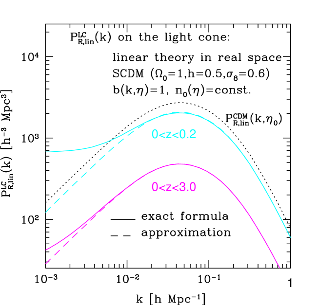
Figure 1: Power spectra of cosmological objects on a light cone, $P^{\rm LC}_{\rm R,lin}(k)$. Upper and lower pairs of curves correspond to the samples of survey depth extending up to $z=0.2$ and $3.0$, respectively (the exact formula eq.[12] in solid lines, and its approximation eq.[16] in dashed lines). For comparison, the power spectrum of the mass fluctuations defined on the constant-time hypersurface at present is plotted in dotted line. For definiteness we adopt SCDM model in which $\Omega_{0}=1$, $\Omega_{\Lambda}=0$, $h=0.5$ and $\sigma_{8}=0.6$

Figure 1 compares the power spectra on a light cone, equations (12) and (16). It should be noted that $P^{\rm LC}_{\rm R,lin}(k)$ in the exact formula becomes significantly larger than $P_{\rm R,lin}(k)$ for $k\lower 2.15277pt\hbox{$\;\buildrel<\over{\sim}\;$}1/r(z_{\rm max})$ with $r(z_{\rm max})$ being the depth of the survey volume. This artifact is not particular to the light-cone effect, but simply originates from the fact that the power on scales comparable to, or larger than, the finite size of the survey volume cannot be properly evaluated.

Thus except for the range $k\ll 1/r(z_{\rm max})$, where the estimate of the power is fairly reliable for a given observational sample, Figure 1 shows that the approximation (16) reproduces the exact formula very accurately. Therefore in what follows, we will incorporate several important effects (redshift-space distortion, nonlinear density and velocity evolution, and the observational selection function) on the basis of the approximation.

While the results in Figure 1 do not include the selection function, i.e., $n_{0}(z)$=constant. is assumed, we also examined the case with the proper selection functions for galaxies and quasars (§4), and made sure that our approximation agrees with the exact formula within several percents at worst. This level of accuracy is sufficiently good in the light of the other approximations employed in describing the nonlinearity of density and velocity fields, most notably, the uncertainty of the model of bias.

3 Redshift-space distortion and nonlinear evolution of density and velocity fields

The results presented in the previous section are unrealistically simplified since we have neglected several important effects including the redshift-space distortion due to the peculiar velocity effect (Kaiser 1987), nonlinear evolution of mass density fluctuations and of peculiar velocity dispersions (finger-of-God), evolution of the bias parameter (e.g., Fry 1996), and the observational selection function which depends on a specific survey strategy. In this section we describe our modeling to the first three effects which are the necessary ingredients in completing the theoretical predictions. The selection function is discussed in the next section. Strictly speaking, inclusion of these effects invalidates the exact derivation of the formula (12) unfortunately. Therefore we implement a phenomenological correction to these effects as described below, but we believe that this procedure is important and useful in practice, especially given the uncertainty of the bias evolution itself.

3.1 Linear redshift-space distortion

The cosmological observation is possible only in redshift space. The redshift-space distortion in linear theory, first discussed by Kaiser (1987), is easily included in our formula for power spectrum on the light cone in real space. In linear theory, the direction–averaged power spectrum in redshift space, $P_{\rm S,lin}(k,z)$ is related to that in real space, $P_{\rm R,lin}(k,z)$, as

$$P_{\rm S,lin}(k,z)=\left[1+{2\over 3}\beta(z)+{1\over 5}\beta^{2}(z)\right]P_{\rm R,lin}(k,z).$$ (18)

The above relation (Kaiser 1987) assumes a distant-observer approximation, and scale-independent linear bias, $b(z)$, as well. Then $\beta(z)$ is defined by

$$\beta(z)={1\over b(z)}{d\ln D_{1}\over d\ln a}.$$ (19)

See Matsubara & Suto (1996), Hamilton (1998) and Paper III for extensive discussion on the redshift-space distortion.

Substituting equation (18) in equation (12) yields the expression for $P^{\rm LC}_{\rm S,lin}(k)$ which is approximated as

$$P^{\rm LC}_{\rm S,lin}(k) \simeq \alpha_{\rm S,lin}(k)P_{\rm R,lin}(k,z=0),$$ (20)

$$\alpha_{\rm S,lin}(k) = {\displaystyle{\int drr^{2}n_{0}^{\rm LC}(r)^{2}D_{1}(\eta_{0}-r)^{2}}b(k;\eta_{0}-r)^{2}\left[1+{2\over 3}\beta(\eta_{0}-r)+{1\over 5}\beta^{2}(\eta_{0}-r)\right]\over{\displaystyle\int drr^{2}{n^{\rm LC}_{0}}(r)^{2}}}.\hskip 14.22636pt$$ (21)

A similar expression for the linear redshift-space distortion on two-point correlation functions is derived in Paper II.

3.2 Nonlinear evolution of density

Nonlinear evolution of mass density field introduces the additional $k$-dependence on the light-cone power spectrum. While the full description of the nonlinear gravitational evolution of density fields is almost impossible, fairly accurate fitting formulae for $P_{\rm R,nl}(k,z)$ have been obtained (e.g., Peacock & Dodds 1994,1996). We attempt to correct for the nonlinear density evolution simply by adopting the fitting formulae, and then obtain an approximate expression for $P^{\rm LC}_{\rm R,nl}(k)$ as follows:

$$P^{\rm LC}_{\rm R,nl}(k) \simeq \alpha_{\rm R,nl}(k)P_{\rm R,lin}(k,z=0),$$ (22)

$$\alpha_{\rm R,nl}(k) = {\displaystyle{\int drr^{2}n_{0}^{\rm LC}(r)^{2}}b(k;\eta_{0}-r)^{2}P_{\rm R,nl}(k,\eta_{0}-r)\over P_{\rm R,lin}(k,z=0){\displaystyle\int drr^{2}{n^{\rm LC}_{0}}(r)^{2}}}.$$ (23)

3.3 Nonlinear redshift-space distortion; finger-of-God effect

Finally an effect of the nonlinear velocity field, finger-of-God, should be taken into account in order to make a testable theoretical prediction. Again this has been extensively discussed for the power spectrum on the constant-time hypersurface (Cole, Fisher & Weinberg 1994; Mo, Jing, & Börner 1997; Paper III; Magira, Jing & Suto 1999). In particular, Cole et al. (1994) proposed the following correction for the finger-of-God effect:

$$P_{\rm S,nl}(k,z)=\left[A(\kappa)+{2\over 3}\beta(z)B(\kappa)+{1\over 5}\beta^{2}(z)C(\kappa)\right]P_{\rm R,nl}(k,z).$$ (24)

If the velocity distribution function is approximated by an exponential model with scale-independent one-dimensional dispersion of the peculiar velocity ${\sigma_{v}}(z)$, which is indicated observationally (Davis & Peebles 1983) and also from numerical simulations (Efstathiou et al. 1988; Ueda, Itoh & Suto 1993; Magira et al. 1999), the above functions are explicitly given by

$$A(\kappa) = {{\rm arctan}(\kappa/\sqrt{2})\over\sqrt{2}\kappa}+{1\over 2+\kappa^{2}},$$ (25)

$$B(\kappa) = {6\over\kappa^{2}}\biggl{(}A(\kappa)-{2\over 2+\kappa^{2}}\biggr{)},$$ (26)

$$C(\kappa) = {-10\over\kappa^{2}}\biggl{(}B(\kappa)-{2\over 2+\kappa^{2}}\biggr{)},$$ (27)

with $\kappa(z)=k{\sigma_{v}}(z)/H_{0}$. On large scales, ${\sigma_{v}}(z)$ can be well approximated by a fitting formula proposed by Mo, Jing & Börner (1997). The validity and limitation of the approximation are discussed in detail by Magira et al. (1999). Combining equation (24) with those fitting formulae, one can compute the nonlinear power spectrum on the light cone in redshift space as

$$P^{\rm LC}_{\rm S,nl}(k) \simeq \alpha_{\rm S,nl}(k)P_{\rm R,lin}(k,z=0),$$ (28)

$$\alpha_{\rm S,nl}(k) = {\displaystyle{\int drr^{2}n_{0}^{\rm LC}(r)^{2}}b(k;\eta_{0}-r)^{2}P_{\rm R,nl}(k,\eta_{0}-r)\left[A(\kappa)+{2\over 3}\beta B(\kappa)+{1\over 5}\beta^{2}C(\kappa)\right]\over P_{\rm R,lin}(k,z=0){\displaystyle\int drr^{2}{n^{\rm LC}_{0}}(r)^{2}}}.\hskip 28.45274pt$$ (29)

4 Predictions of power spectra on the light cone for the future redshift surveys

4.1 Selection function for galaxies and quasars

In properly predicting the power spectra on the light cone, the selection function should be specified. In this subsection, we describe the selection functions of galaxies and quasars with the upcoming SDSS spectroscopic samples in mind.

For galaxies, we adopt a B-band luminosity function of the APM galaxies (Loveday et al. 1992) fitted to the Schechter function:

$$\phi(L)dL=\phi^{*}\biggl{(}{L\over L^{*}}\biggr{)}^{\alpha}\exp\biggl{(}-{L\over L^{*}}\biggr{)}d\biggl{(}{L\over L^{*}}\biggr{)},$$ (30)

with $\phi^{*}=1.40\times 10^{-2}h^{3}{\rm Mpc}^{-3}$, $\alpha=-0.97$, and $M_{B}^{*}=-19.50+5\log_{10}h$. Then the comoving number density of galaxies at $z$ which are brighter than the limiting magnitude $B_{\rm lim}$ is given by

$$n_{0}(z,<B_{\rm lim})=\int_{L(B_{\rm lim},z)}^{\infty}\phi(L)dL=\phi^{*}\Gamma[(\alpha+1,x(B_{\rm lim},z)],$$ (31)

where

$$x(B_{\rm lim},z)\equiv{L(B_{\rm lim},z)\over L^{*}}=\left[{d_{L}(z)\over 1h^{-1}{\rm Mpc}}\right]^{2}10^{2.2-0.4B_{\rm lim}},$$ (32)

and $\Gamma[\nu,x]$ is the incomplete Gamma function.

For quasars, we compute a selection function for B-band magnitude limited samples following Paper I on the basis of the luminosity function by Wallington & Narayan (1993; see also Nakamura & Suto 1997).

4.2 Models and predictions

For definiteness, we consider SCDM (standard cold dark matter) and LCDM (Lambda cold dark matter) models, which have $(\Omega_{0},\Omega_{\Lambda},h,\sigma_{8})$ $=(1.0,0.0,0.5,0.6)$ and $(0.3,0.7,0.7,1.0)$, respectively. These sets of cosmological parameters are chosen so as to reproduce the observed cluster abundance (Kitayama & Suto 1997). We use the fitting formulae of Peacock & Dodds (1996) and Mo, Jing, & Börner (1997) for the nonlinear power spectrum $P_{\rm R,nl}(k)$ and the peculiar velocity dispersions ${\sigma_{v}}$, respectively.

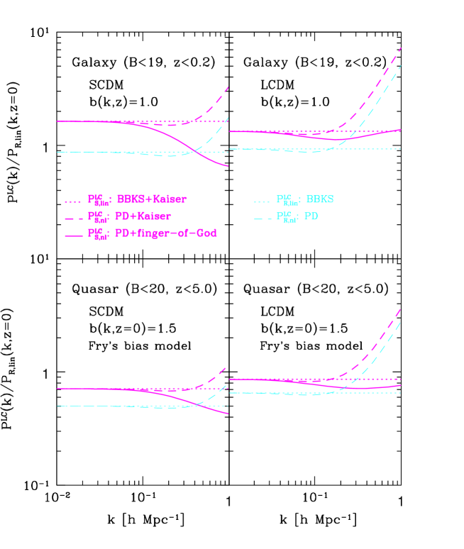
Figure 2: Power spectra on the light cone, $P^{\rm LC}(k)$, for various models, divided by $P_{\rm R,lin}(k,z=0)$, the corresponding linear power spectrum on the constant-time hypersurface in real space at $z=0$. Upper panels assume a galaxy sample with $B<19$ and $z<0.2$, while lower panels are for a quasar sample with $B<20$ and $z<5$, both of which roughly correspond to the upcoming SDSS spectroscopic samples. Left and right panels plot the results in SCDM and LCDM models, respectively. Thick and thin lines represent $P^{\rm LC}(k)$ measured in redshift and real spaces.

Figure 2 plots the theoretical predictions for power spectra on the light cone. We adopt the B-band limiting magnitude $19$ and $20$ for galaxies and quasars, respectively, so as to roughly match the SDSS and 2dF spectroscopic samples. For illustrative purposes, the results are divided by the corresponding linear power spectrum on the constant-time hypersurface in real space at $z=0$, $P_{\rm R,lin}(k,z=0)$. For simplicity we adopt a scale-independent linear bias model of Fry (1996); $b(k,z=0)=1$ and $1.5$ for galaxies and quasars ($p=1$ in eq.[33] below). Purely linear theory predictions, $P^{\rm LC}_{\rm S,lin}(k)$, are plotted in dotted lines, which use the CDM transfer function by Bardeen et al.(1986; BBKS) and the linear redshift-space distortion (20) by Kaiser (1987). We show two different versions of $P^{\rm LC}_{\rm S,nl}(k)$ ; both adopt the Peacock & Dodds (1996; PD) nonlinear spectrum, one, plotted in dashed lines, uses linear redshift-space distortion, and the other (solid lines) uses the nonlinear model (28) with the velocity dispersion formula by Mo, Jing & Börner (1997).

In linear regime, the light-cone effect suppresses the amplitude of spectrum in real space due to the smaller fluctuation at larger $z$ unless the possible evolution of bias exceeds the linear growth rate of the mass fluctuations. The redshift-space distortion, on the other hand, tends to increase the observable power spectrum in redshift space. Thus the overall effect of the linear redshift-space distortion on the light cone is to increase (decrease) the amplitude of $P^{\rm LC}_{\rm S,lin}(k)$ for galaxy (quasar) samples in a $k$-independent manner.

The situation becomes complicated in nonlinear regimes, which produces the additional $k$-dependent behavior. While the nonlinear evolution of density field enhances the amplitude of both $P^{\rm LC}_{\rm R,nl}(k)$ and $P^{\rm LC}_{\rm S,nl}(k)$ relative to their counterparts in linear theory , the suppression due to the finger-of-God is much stronger. Consequently $P^{\rm LC}_{\rm S,nl}(k)$ is smaller than $P^{\rm LC}_{\rm S,lin}(k)$ for any $k$, and in fact the suppression is stronger for larger $k$. Since recent numerical simulations (Mo, Jing, & Börner 1997; Jing 1998; Suto et al. 1999; Magira et al. 1999) confirmed that the nonlinear fitting formulae of density and velocity fields are accurate and reliable within several percents, these conclusions are generic as long as the bias is time-independent. The bias, however, is predicted to show strong time evolution. Furthermore the realistic bias is expected to be neither time-independent nor linear (Fry 1996; Mo & White 1996); it may even not be deterministic (Tegmark & Peebles 1998; Dekel & Lahav 1999; Taruya, Koyama & Soda 1999). We will discuss this problem in detail elsewhere, and focus on the effect of time-evolution of bias in the next subsection.

4.3 Dependence on time-evolution of bias

As discussed in previous subsection, the most uncertain aspect of the theoretical predictions of $P^{\rm LC}(k)$ is the model of bias. Since it is unlikely that any reliable theoretical model for bias is established in near future, all that one can try is to explore the possible effects by adopting a simple parametric model. While several phenomenological models of evolution of bias have been proposed in the literature (e.g., Moscardini, et al. 1998; Matarrese, et al. 1997), we adopt the following simple model:

$$b(\eta)=1+{1\over[D_{1}(\eta)]^{p}}[b_{0}-1],$$ (33)

with $b_{0}\equiv b(\eta_{0})$ is the bias parameter at present. When the constant index $p$ is unity, the model reproduces the time-evolution of the lowest-order bias coefficient which is discussed by Fry (1996) on the basis of the continuity equation of mass and galaxy density fields.

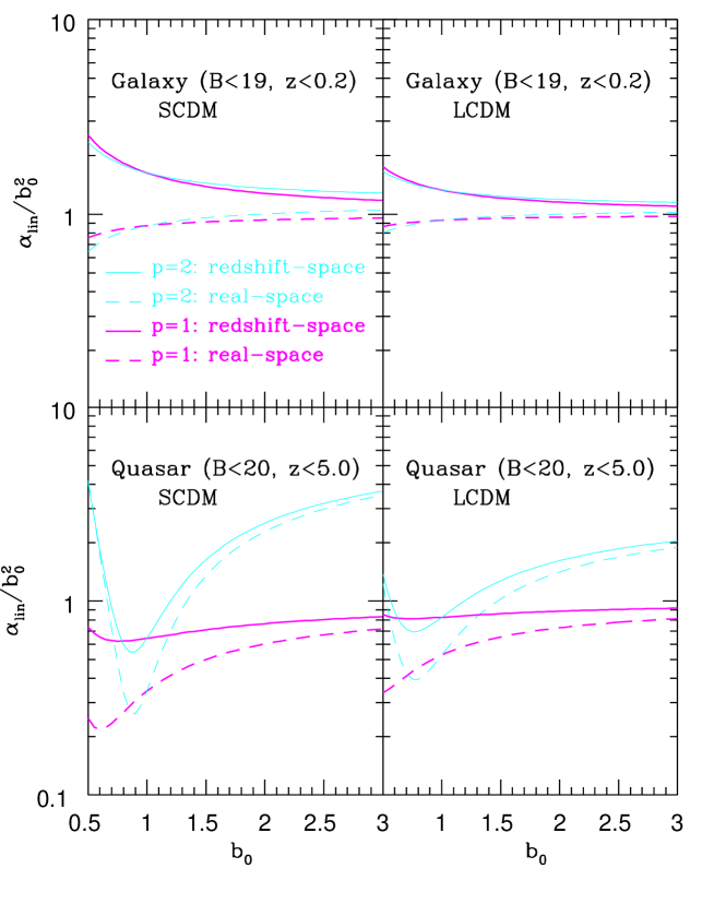
Figure 3: $\alpha_{\rm R,lin}/b_{0}^{2}$ and $\alpha_{\rm S,lin}/b_{0}^{2}$ as a function of the linear bias parameter at present $b_{0}$. Solid and dashed lines represent the ratio measured in redshift and real spaces, respectively; $p=1$ in thick and $p=2$ in thin lines. The model with $p=1$ corresponds to the bias evolution model of Fry (1996).

Figure 3 plots $\alpha_{\rm R,lin}/b_{0}^{2}$ and $\alpha_{\rm S,lin}/b_{0}^{2}$ for $p=1$ (Fry’s model) and $2$ (regarded as an extreme example for comparison) as a function of $b_{0}$. The selection functions for the galaxy and quasar samples are identical to those adopted in Figure 2. For shallow samples like the SDSS galaxies, theoretical predictions are fairly insensitive to the applied model of evolution of bias; the cosmological light-cone effect on these samples is dominated by the redshift-space distortion. For deeper samples, however, the amplitude is very sensitive to the evolution of bias; especially when the bias evolves faster than the linear growth rate ($p>1$), the redshift-space distortion becomes relatively negligible on linear scales.

5 Conclusions

In this paper we have developed a theoretical formulation to compute the power spectrum of cosmological objects on the light-cone hypersurface. On the basis of the exact formula which works in linear theory and in real space, we have obtained a useful approximate expression valid on scales less than the survey volume size (Further discussions for the validity of the approximation will be given elsewhere; Nishioka & Yamamoto 1999b). In linear theory, the light-cone effect simply suppresses (in general) the amplitude of the observable power spectrum (as in the case of the two-point correlation functions; see Papers I, II and III). Then we improved the approximate formula by including the nonlinear evolution of density fields, and linear and nonlinear redshift-space distortion phenomenologically but in a manner fully consistent with the recent numerical simulations. These nonlinearities produce the additional scale-dependence in the power spectrum on the light cone compared with those defined on the constant-time hypersurface.

Applying this expression to the galaxy and quasar samples selected so as to match the upcoming SDSS spectroscopic samples, for instance, we have quantitatively evaluated the degree of the light-cone effect. With these example, we have demonstrated that we have developed a fairly reliable and useful method to compute the power spectrum on the light cone given an evolution model of bias. In fact, it is clear that the evolution of bias sensitively changes the behavior of the power spectrum on the light cone, especially for quasar samples. While our present analysis assumes the simplest bias model, linear bias, we plan to extend our formulation for the general bias model including the stochastic bias models (Dekel & Lahav 1999; Taruya, Koyama, & Soda 1999)

We thank Y.Kojima, T.Matsubara and M.Sasaki for useful discussions and comments, and Y.P.Jing and H.Magira for providing numerical routines to compute fitting formulae for nonlinear density and velocity fields. This research was supported in part by the Grants-in-Aid by the Ministry of Education, Science, Sports and Culture of Japan to RESCEU (07CE2002) and to K.Y. (11640280), by the Supercomputer Project (No.98-35, and No.99-52) of High Energy Accelerator Research Organization (KEK) in Japan, and by the Inamori Foundation.

REFERENCES

Bardeen, J.M., Bond, J.R, Kaiser, N., & Szalay, A.S. 1986, ApJ, 304, 15 (BBKS)

Cole, S., Fisher, K. B., & Weinberg, D. H. 1995, MNRAS, 275, 515

Davis, M. , & Peebles, P.J.E. 1983, ApJ, 267, 465

Dekel, A. , & Lahav, O. 1999, ApJ, 520, 24

de Laix, A. A. , & Starkman, G. D. 1998, MNRAS, 299, 977

Efstathiou, G., Frenk, C.S., White, S.D.M. , & Davis, M. 1988, MNRAS, 235, 715

Feldman, H. A., Kaiser, N., & Peacock, A. A. 1994, ApJ, 426, 23

Fry, J. N. 1996, ApJ, 461, L65

Hamilton, A.J.S. 1998, in “ The Evolving Universe. Selected Topics on Large-Scale Structure and on the Properties of Galaxies”, (Kluwer: Dordrecht), p.185.

Jing, Y.P. 1998, ApJ, 503, L9

Kaiser, N. 1987, MNRAS, 227, 1

Kitayama, T. , & Suto, Y. 1997, ApJ, 490, 557

Loveday,J., Peterson, B.A., Efstathiou, G., & Maddox, S.J. 1992, ApJ, 390, 338

Magira, H., Jing, Y.P., & Suto, Y. 1999, ApJ, in press.

Matarrese, S., Coles, P., Lucchin, F., & Moscardini, L. 1997, MNRAS, 286, 115

Matsubara, T. , & Suto, Y. 1996, ApJ, 470, L1

Matsubara, T. , Suto, Y., & Szapudi,I. 1997, ApJ, 491, L1

Mo, H.J., Jing, Y.P. , & Börner, G. 1997, MNRAS, 286, 979

Mo, H.J. , & White, S.D.M. 1996, MNRAS, 282, 347

Moessner, R., Jain, B., & Villumsen, J. V. 1998, MNRAS, 294, 291

Moscardini, L., Coles, P., Lucchin, F., & Matarrese, S. 1998 , MNRAS, 299, 95

Nakamura, T.T., Matsubara, T., & Suto, Y. 1998, ApJ, 494, 13

Nakamura, T.T., & Suto, Y. 1997, Prog. Theor. Phys., 97, 49

Nishioka, H. , & Yamamoto, K. 1999a, ApJ, 520, 426(Paper II)

Nishioka, H. , & Yamamoto, K. 1999b, in preparation.

Peacock, J.A. , & Dodds, S.J. 1994, MNRAS, 267, 1020

Peacock, J.A. , & Dodds, S.J. 1996, MNRAS, 280, L19 (PD)

Suto, Y., Magira, H., Jing, Y. P., Matsubara, T., & Yamamoto, K. 1999, Prog.Theor.Phys.Suppl., 133, 183 (Paper III, astro-ph/9901179)

Taruya, A., Koyama, K., & Soda, J. 1999, ApJ, 510, 541

Tegmark, M. , & Peebles, P.J.E. 1998, ApJ, 500, L79

Ueda, H., Itoh, M., & Suto, Y. 1993, ApJ, 408, 3

Wallington, S. , & Narayan, R. 1993, ApJ, 403, 517

Yamamoto, K. , & Suto, Y. 1999, ApJ, 517, 1 (Paper I)

APPENDIX

Appendix A Linear theory derivation of the exact formula of the light-cone power spectrum $P^{\rm LC}_{\rm R,lin}(k)$ in real space

In this appendix, we outline the derivation of equation (12) from equation (11):

$$P^{\rm LC}_{\rm R,lin}(k)={\displaystyle\int d^{3}{\bf r}_{1}\int d^{3}{\bf r}_{2}\bigl{<}[n^{\rm LC}(r_{1},{\vec{\gamma}}_{1})-n_{s}^{\rm LC}(r_{1},{\vec{\gamma}}_{1})][n^{\rm LC}(r_{2},{\vec{\gamma}}_{2})-n_{s}^{\rm LC}(r_{2},{\vec{\gamma}}_{2})]\bigr{>}e^{i{\bf k}\cdot({\bf r}_{1}-{\bf r}_{2})}\over\displaystyle\int d^{3}{\bf r}n_{0}^{\rm LC}(r)^{2}}.\hskip 11.38092pt$$ (A1)

With equations (5) and (8),the numerator of the integrand in equation (A1) becomes

$$\bigl{<}[n^{\rm LC}(r_{1},{\vec{\gamma}}_{1})-n_{s}^{\rm LC}(r_{1},{\vec{\gamma}}_{1})][n^{\rm LC}(r_{2},{\vec{\gamma}}_{2})-n_{s}^{\rm LC}(r_{2},{\vec{\gamma}}_{2})]\bigr{>}$$

$$\hskip 99.58464pt={n^{\rm LC}_{0}}(r_{1}){n^{\rm LC}_{0}}(r_{2})\bigl{<}\Delta(\eta_{0}-r_{1},r_{1},{\vec{\gamma}}_{1})\Delta(\eta_{0}-r_{2},r_{2},{\vec{\gamma}}_{2})\bigr{>}.$$ (A2)

We expand the fluctuations $\Delta(\eta,r,\vec{\gamma})$ in equation (4) as

$$\Delta(\eta,\chi,\vec{\gamma})=\int^{\infty}_{0}dk\sum_{l,m}\Delta_{klm}(\eta){\cal Y}_{klm}(\chi,{\vec{\gamma}}),$$ (A3)

where ${\cal Y}_{klm}(\chi,{\vec{\gamma}})$ is the normalized harmonics on the flat space:

$${\cal Y}_{klm}(\chi,{\vec{\gamma}})={\sqrt{2\over\pi}}kj_{l}(k\chi)Y_{lm}(\Omega_{\vec{\gamma}}),$$ (A4)

with $j_{l}(x)$ being the spherical Bessel function and $Y_{lm}(\Omega_{\vec{\gamma}})$ being the spherical harmonics on a unit two-sphere. To proceed further, we adopt two assumptions; a linear bias model in Fourier space:

$$\Delta_{klm}(\eta)=b(k;\eta)\delta^{(c)}_{klm}(\eta),$$ (A5)

and linear growth of the density fluctuations:

$$\delta^{(c)}_{klm}(\eta)=\delta^{(c)}_{klm}(\eta_{0})D_{1}(\eta),$$ (A6)

with $D_{1}(\eta)$ being the linear growth rate normalized to be $D_{1}(\eta_{0})=1$. In the above expressions, we denote the density fluctuations by $\delta^{(c)}_{klm}(\eta)$ with CDM density fluctuation specifically in mind, although not essential at all.

Then the power spectrum of mass density fluctuations at present, $P_{\rm R,lin}(k,\eta_{0})$, is defined through

$$\bigl{<}\delta^{(c)}_{k_{1}l_{1}m_{1}}(\eta_{0})\delta^{(c)*}_{k_{2}l_{2}m_{2}}(\eta_{0})\bigr{>}=P_{\rm R,lin}(k_{1},\eta_{0})\delta(k_{1}-k_{2})\delta_{l_{1}l_{2}}\delta_{m_{1}m_{2}}.$$ (A7)

Substituting equations (A3) to (A7), one can write the third term in equation (A2) as

$$\bigl{<}\Delta(\eta_{0}-r_{1},r_{1},{\vec{\gamma}}_{1})\Delta(\eta_{0}-r_{2},r_{2},{\vec{\gamma}}_{2})\bigr{>}$$

$$\hskip 56.9055pt={2\over\pi}\int^{\infty}_{0}dk_{1}k_{1}^{2}P_{\rm R,lin}(k_{1},\eta_{0})b(k_{1};\eta_{0}-r_{1})b(k_{2};\eta_{0}-r_{2})D_{1}(\eta_{0}-r_{1})D_{1}(\eta_{0}-r_{2})$$

$$\hskip 85.35826pt\times\sum_{l,m}j_{l}(k_{1}r_{1})j_{l}(k_{1}r_{2})Y^{*}_{lm}(\Omega_{\vec{\gamma}_{1}})Y_{lm}(\Omega_{\vec{\gamma}_{2}})~{}.$$ (A8)

Using the expansion of the plane wave in terms of the spherical harmonics:

$$e^{i{\bf k}\cdot{\bf r}}=4\pi\sum_{lm}i^{l}j_{l}(kr)Y_{lm}(\Omega_{\vec{\gamma}})Y^{*}_{lm}(\Omega_{\hat{\bf k}}),$$ (A9)

and equation (A8), equation (A1) is explicitly written as

$$P^{\rm LC}_{\rm R,lin}(k) = \left[\int d^{3}{\bf r}{n^{\rm LC}_{0}}(r)^{2}\right]^{-1}\int dr_{1}r_{1}^{2}\int d\Omega_{\vec{\gamma}_{1}}\int dr_{2}r_{1}^{2}\int d\Omega_{\vec{\gamma}_{2}}{n^{\rm LC}_{0}}(r_{1}){n^{\rm LC}_{0}}(r_{2})$$ (A10)

$$\times{2\over\pi}\int^{\infty}_{0}dk_{1}k_{1}^{2}P_{\rm R,lin}(k_{1},\eta_{0})b(k_{1};\eta_{0}-r_{1})b(k_{1};\eta_{0}-r_{2})D_{1}(\eta_{0}-r_{1})D_{1}(\eta_{0}-r_{1})$$

$$\times\sum_{l,m}j_{l}(k_{1}r_{1})j_{l}(k_{1}r_{2})Y^{*}_{lm}(\Omega_{\vec{\gamma}_{1}})Y_{lm}(\Omega_{\vec{\gamma}_{2}})$$

$$\times~{}4\pi\sum_{L_{1}M_{1}}i^{L_{1}}j_{L_{1}}(kr_{1})Y_{L_{1}M_{1}}(\Omega_{\vec{\gamma}_{1}})Y^{*}_{L_{1}M_{1}}(\Omega_{\hat{\bf k}})$$

$$\times~{}4\pi\sum_{L_{2}M_{2}}i^{-L_{2}}j_{L_{2}}(kr_{2})Y^{*}_{L_{2}M_{2}}(\Omega_{\vec{\gamma}_{2}})Y_{L_{2}M_{2}}(\Omega_{\hat{\bf k}}).$$

Integrating equation (A10) over $\Omega_{\vec{\gamma}_{1}}$ and $\Omega_{\vec{\gamma}_{2}}$ results in

$$P^{\rm LC}_{\rm R,lin}(k)=\left[\int d^{3}{\bf r}{n^{\rm LC}_{0}}(r)^{2}\right]^{-1}\int dr_{1}r_{1}^{2}\int dr_{2}r_{2}^{2}{n^{\rm LC}_{0}}(r_{1}){n^{\rm LC}_{0}}(r_{2})$$

$$\hskip 42.67912pt\times{2\over\pi}\int^{\infty}_{0}dk_{1}k_{1}^{2}P_{\rm R,lin}(k_{1},\eta_{0})b(k_{1};\eta_{0}-r_{1})b(k_{1};\eta_{0}-r_{2})D_{1}(\eta_{0}-r_{1})D_{1}(\eta_{0}-r_{2})$$

$$\hskip 42.67912pt\times(4\pi)^{2}\sum_{l,m}j_{l}(k_{1}r_{1})j_{l}(k_{1}r_{2})j_{l}(kr_{1})j_{l}(kr_{2})Y_{lm}(\Omega_{\hat{\bf k}})Y^{*}_{lm}(\Omega_{\hat{\bf k}}).$$ (A11)

Using the mathematical formula:

$$\sum^{l}_{m=-l}Y_{lm}(\Omega)Y_{lm}(\Omega^{\prime})={2l+1\over 4\pi}P_{l}(\cos\theta),$$ (A12)

one can simplify equation (A11) as follows:

$$P^{\rm LC}_{\rm R,lin}(k)=\left[\int drr^{2}{n^{\rm LC}_{0}}(r)^{2}\right]^{-1}\int dr_{1}r_{1}^{2}\int dr_{2}r_{2}^{2}{n^{\rm LC}_{0}}(r_{1}){n^{\rm LC}_{0}}(r_{2})D_{1}(\eta_{0}-r_{1})D_{1}(\eta_{0}-r_{2})$$

$$\hskip 42.67912pt\times{2\over\pi}\int^{\infty}_{0}dk_{1}k_{1}^{2}P_{\rm R,lin}(k_{1},\eta_{0})b(k_{1};\eta_{0}-r_{1})b(k_{1};\eta_{0}-r_{2})$$

$$\hskip 42.67912pt\times\sum_{l}(2l+1)j_{l}(k_{1}r_{1})j_{l}(kr_{1})j_{l}(k_{1}r_{2})j_{l}(kr_{2}).$$ (A13)

Applying the formula:

$$j_{l}(a\lambda)j_{l}(b\lambda)={1\over 2\lambda}\int^{1}_{-1}dx(a^{2}+b^{2}-2abx)^{-{1\over 2}}\sin[\lambda(a^{2}+b^{2}-2abx)^{1\over 2}]P_{l}(x)$$ (A14)

and then

$$\delta(x-x^{\prime})=\sum_{n}{2n+1\over 2}P_{n}(x)P_{n}(x^{\prime}),$$ (A15)

equation (A13) is written as

$$P^{\rm LC}_{\rm R,lin}(k) = \left[\int drr^{2}{n^{\rm LC}_{0}}(r)^{2}\right]^{-1}\int dr_{1}r_{1}^{2}\int dr_{2}r_{2}^{2}{n^{\rm LC}_{0}}(r_{1}){n^{\rm LC}_{0}}(r_{2})D_{1}(\eta_{0}-r_{1})D_{1}(\eta_{0}-r_{2})$$ (A16)

$$\hskip 14.22636pt\times{2\over\pi}\int^{\infty}_{0}dk_{1}k_{1}^{2}P_{\rm R,lin}(k_{1},\eta_{0})b(k_{1};\eta_{0}-r_{1})b(k_{1};\eta_{0}-r_{2})\sum_{l}(2l+1)$$

$$\hskip 14.22636pt\times{1\over 2k_{1}}\int^{1}_{-1}dx_{1}(r_{1}^{2}+r_{2}^{2}-2r_{1}r_{2}x_{1})^{-{1\over 2}}\sin[k_{1}(r_{1}^{2}+r_{2}^{2}-2r_{1}r_{2}x_{1})^{1\over 2}]P_{l}(x_{1})$$

$$\hskip 14.22636pt\times{1\over 2k}\int^{1}_{-1}dx_{2}(r_{1}^{2}+r_{2}^{2}-2r_{1}r_{2}x_{2})^{-{1\over 2}}\sin[k(r_{1}^{2}+r_{2}^{2}-2r_{1}r_{2}x_{2})^{1\over 2}]P_{l}(x_{2})$$

$$= \left[\int drr^{2}{n^{\rm LC}_{0}}(r)^{2}\right]^{-1}\int dr_{1}r_{1}^{2}\int dr_{2}r_{2}^{2}{n^{\rm LC}_{0}}(r_{1}){n^{\rm LC}_{0}}(r_{2})D_{1}(\eta_{0}-r_{1})D_{1}(\eta_{0}-r_{2})$$

$$\hskip 14.22636pt\times{1\over\pi k}\int^{\infty}_{0}dk_{1}k_{1}P_{\rm R,lin}(k_{1},\eta_{0})b(k_{1};\eta_{0}-r_{1})b(k_{1};\eta_{0}-r_{2})$$

$$\hskip 14.22636pt\times\int^{1}_{-1}dx{\sin[k_{1}(r_{1}^{2}+r_{2}^{2}-2r_{1}r_{2}x)^{1/2}]\sin[k(r_{1}^{2}+r_{2}^{2}-2r_{1}r_{2}x)^{1/2}]\over r_{1}^{2}+r_{2}^{2}-2r_{1}r_{2}x}.$$

Finally changing the variable $x$ to $y\equiv(r_{1}^{2}+r_{2}^{2}-2r_{1}r_{2}x)^{1/2}$, equation (A16) reduces to

$$P^{\rm LC}_{\rm R,lin}(k)=\left[\int drr^{2}{n^{\rm LC}_{0}}(r)^{2}\right]^{-1}\int dr_{1}r_{1}\int dr_{2}r_{2}{n^{\rm LC}_{0}}(r_{1}){n^{\rm LC}_{0}}(r_{2})D_{1}(\eta_{0}-r_{1})D_{1}(\eta_{0}-r_{2})$$

$$\hskip 14.22636pt\times{1\over\pi k}\int^{\infty}_{0}dk_{1}k_{1}P_{\rm R,lin}(k_{1},\eta_{0})b(k_{1};\eta_{0}-r_{1})b(k_{1};\eta_{0}-r_{2})\int^{r_{1}+r_{2}}_{|r_{1}-r_{2}|}dy{\sin k_{1}y\sin ky\over y}.$$ (A17)

Rewriting the last integral of the above expression in terms of the the cosine integral function:

$$C_{i}(x)\equiv-\int^{\infty}_{x}dt{\cos t\over t},$$ (A18)

equation (A17) yields the final expression (12), namely,

$$P^{\rm LC}_{\rm R,lin}(k)=\left[\int drr^{2}{n^{\rm LC}_{0}}(r)^{2}\right]^{-1}\int dr_{1}r_{1}\int dr_{2}r_{2}{n^{\rm LC}_{0}}(r_{1}){n^{\rm LC}_{0}}(r_{2})D_{1}(\eta_{0}-r_{1})D_{1}(\eta_{0}-r_{2})$$

$$\hskip 42.67912pt\times{1\over 2\pi k}\int^{\infty}_{0}dk_{1}k_{1}P_{\rm R,lin}(k_{1},\eta_{0})b(k_{1};\eta_{0}-r_{1})b(k_{1};\eta_{0}-r_{2})\Pi(r_{1},r_{2},k_{1},k),$$ (A19)

where

$$\Pi(r_{1},r_{2},k_{1},k)=-C_{i}\bigl{(}|r_{1}-r_{2}||k_{1}-k|\bigr{)}+C_{i}\bigl{(}|r_{1}-r_{2}|(k_{1}+k)\bigr{)}$$

$$\hskip 85.35826pt+C_{i}\bigl{(}(r_{1}+r_{2})|k_{1}-k|\bigr{)}-C_{i}\bigl{(}(r_{1}+r_{2})(k_{1}+k)\bigr{)}~{}.$$ (A20)