Two measures of the shape of the Milky Way’s dark halo

Abstract

In order to test the reliability of determinations of the shapes of galaxies’ dark matter halos, we have made such measurements for the Milky Way by two independent methods. First, we have combined the measurements of the over-all mass distribution of the Milky Way derived from its rotation curve and the measurements of the amount of dark matter in the solar neighborhood obtained from stellar kinematics to determine the flattening of the dark halo. Second, we have used the established technique based on the variation in thickness of the Milky Way’s Hi layer with radius: by assuming that the Hi gas is in hydrostatic equilibrium in the gravitational potential of a galaxy, one can use the observe flaring of the gas layer to determine the shape of the dark halo.

These techniques are found to produce a consistent estimate for the flattening of the dark matter halo, with a shortest-to-longest axis ratio of $q\sim 0.8$, but only if one adopts somewhat non-standard values for the distance to the Galactic centre, $R_{0}$, and the local Galactic rotation speed, $\Theta_{0}$. For consistency, one requires values of $R_{0}\la 7.6\,{\rm kpc}$ and $\Theta_{0}\la 190\,{\rm km}\,{\rm s}^{-1}$. The results depend on the Galactic constants because the adopted values affect both distance measurements within the Milky Way and the shape of the rotation curve, which, in turn, alter the inferred halo shape. Although differing significantly from the current IAU-sanctioned values, these upper limits are consistent with all existing observational constraints.

If future measurements confirm these lower values for the Galactic constants, then the validity of the gas layer flaring method will be confirmed. Further, dark matter candidates such as cold molecular gas and massive decaying neutrinos, which predict very flat dark halos with $q\la 0.2$, will be ruled out. Conversely, if the Galactic constants were found to be close to the more conventional values, then there would have to be some systematic error in the methods for measuring dark halo shapes, so the existing modeling techniques would have to be viewed with some scepticism.

1 Introduction

The speed at which spiral galaxies rotate remains relatively constant out to large radii [e.g., Rubin, Ford & Thonnard 1980, Bosma 1981], which implies that they contain large amounts of dark matter. The nature of this material remains obscure, but one key diagnostic is provided by the shape of the dark matter halo, as quantified by its shortest-to-longest axis ratio, $q=c/a$. The roundest halos with $q\sim 0.8$ are predicted by galaxy formation models in which hot dark matter is dominant [Peebles 1993]. Cosmological cold dark matter simulations typically result in triaxial dark halos [Warren et al. 1992] while the inclusion of gas dynamics in the simulations results in somewhat flattened, oblate halos [Katz & Gunn 1991, Udry & Martinet 1994, Dubinski 1994] with $q=0.5\pm 0.15$ [Dubinski 1994]. Models for other dark matter candidates such as cold molecular gas [Pfenniger, Combes & Martinet 1994] and massive decaying neutrinos [Sciama 1990] require halos as flat as $q\sim 0.2$. Clearly, the determination of $q$ for real galaxies offers a valuable test for discriminating between these cosmological models.

Figure 1: A summary of the existing estimates of galaxies’ dark matter halo shapes as parameterized by their shortest-to-longest axis ratio, $q$. For each individual galaxy we indicate the identification and technique used to determine the halo’s flattening: 1) Flaring gas layer [Olling 1996b, Becquaert, Combes & Viallefond 1997]; 2) Warping gas layer [Hofner & Sparke 1994]; 3) X-ray isophotes, [Buote & Canizares 1998]; 4) Polar ring galaxies [Arnaboldi et al. 1993, Sackett et al. 1994, Sackett & Pogge 1995]; 5) precessing dusty disk [Steiman-Cameron, Kormendy & Durisen 1992]. The dotted line shows the predicted distribution for the shapes of halos in a cold dark matter cosmology ($q=0.5\pm 0.15$; Dubinski 1994).

In Fig. 1, we summarize the existing estimates of halo shape, derived using a variety of techniques. It is evident from this figure that there is only a very limited amount of data available for measuring the distribution of $q$ in galaxies. Rather more worrying, though, is the fact that different techniques seem to yield systematically different answers. The warping gas layer method, in which the shape of the halo is inferred by treating any warp in a galaxy’s gas layer as a bending mode in a flattened potential [Hofner & Sparke 1994], seems to imply that dark halos are close to spherical, with $q\ga 0.8$. Conversely, the flaring gas layer technique, which determines the halo shape by assuming that the gas layer is in hydrostatic equilibrium in the galaxy’s gravitational potential and uses the thickness of the layer as a diagnostic for the distribution of mass in the galaxy [Olling 1996b], yields much flatter halo shape estimates with $q\la 0.4$. Although the numbers involved are rather small, there do seem to be real differences between the results obtained by the different methods. Thus, either these techniques are being applied to systematically different classes of galaxy, or at least some of the methods are returning erroneous results.

In order to determine which techniques are credible, we really need to apply several methods to a single galaxy, to see which produce consistent answers. As a first step towards such cross-calibration, this paper compares the shape of our own galaxy’s dark matter halo as inferred by two distinct techniques:

1. Stellar kinematics. Our position within the Milky Way means that we have access to information for this galaxy that cannot be obtained from other systems. In particular, it is possible to measure the total column density of material near the Sun using stellar kinematics. After subtracting off the other components, we can infer the local column density of dark matter. By comparing this density close to the plane of the Galaxy to the over-all mass as derived from its rate of rotation, we can obtain a direct measure of the shape of the halo.

2. The flaring gas layer method. As outlined above, this technique assumes that the Hi emission in the Milky Way comes from gas in hydrostatic equilibrium in the Galactic potential, from which the shape of the dark halo is inferred. Since the results of previous applications of this method give results somewhat out of line with the other techniques, it is important to assess the method’s credibility.

As well as providing a check on the validity of the flaring gas layer method, these analyses will also provide another useful datum on the rather sparsely populated Fig. 1.

The remainder of the paper is laid out as follows. Both of the above methods rely on knowledge of the Milky Way’s rotation velocity as a function of Galactic radius – its “rotation curve” – so Section 2 summarizes the data available for estimating this quantity, and the dependence of the inferred rotation curve on the assumed distance to the Galactic centre and local rotation velocity. The analysis of the shape of the dark halo requires that we decompose the Milky Way into its visible and dark matter components, so Section 3 discusses the construction of a set of models consistent with both the photometric properties of the Galaxy, and its mass properties as inferred from the rotation curve. In Section 4 we show how these mass models can be combined with the local stellar kinematic measurements to determine the shape of the dark halo. Section 5 presents the application of the gas layer flaring technique to the mass models. Section 6 combines the results derived by the two techniques and assesses their consistency. The broader conclusions of this work are drawn in Section 7.

2 The observed rotation curve

Our position within the Milky Way complicates the geometry when studying its structure and kinematics. It is therefore significantly harder to determine our own galaxy’s rotation curve, $\Theta(R)$, than it is to derive those for external systems. More directly accessible to observation than $\Theta(R)$ is the related quantity

$$W(R)=R_{0}\left[{\Theta(R)\over R}-{\Theta_{0}\over R_{0}}\right],$$ (1)

where $R_{0}$ and $\Theta_{0}$ are the distance to the Galactic centre and the local circular speed. If one assumes that material in the galaxy is in purely circular motion, then some simple geometry shows that, for an object at Galactic coordinates $\{l,b\}$ with a line-of-sight velocity $v_{\rm los}$,

$$W={v_{\rm los}\over\sin l\cos b}$$ (2)

(Binney & Merrifield 1998, §9.2.3). Thus, if one measures the line-of-sight velocities for a series of objects at some radius $R$ in the Galaxy, one has an estimate for $W(R)$. By adopting values for $R_{0}$ and $\Theta_{0}$, one can then use equation (1) to determine the rotation speed at that radius.

In practice, the difficulty lies in knowing the Galactic radii of the objects one is looking at. One solution is to look at standard candles, whose distances can be estimated, and hence whose radii in the Galaxy can be geometrically derived. Alternatively, one can select the subset of some tracer – usually Hi or H₂ gas – whose line-of-sight velocities and Galactic coordinates places it at the same value of $W$, and hence at the same radius. One can then use the properties of this cylindrical slice through the Galaxy to infer its radius. For example, in the inner Galaxy, all the material in a ring of radius $R$ will lie at Galactic longitudes of less than $l_{\rm max}=\sin^{-1}(R/R_{0})$, so one can use the extent of the emission on the sky of each $W$-slice to infer its radius – an approach traditionally termed the “tangent point method” [see, for example, Malhotra (1994,1995)]. At radii greater than $R_{0}$ this method is no longer applicable as the emission will be visible at all values of $l$. However, by assuming that the thickness of the gas layer does not vary with azimuth, one can use the observed variation in the angular thickness of the layer with Galactic longitude to estimate the radii of such $W$ slices (Merrifield 1992).

For the remainder of this paper, we use Malhotra’s (1994, 1995) tangent point analysis to estimate $W(R)$ in the inner Galaxy. For the outer Galaxy, we have combined Merrifield’s (1992) data with Brand & Blitz’s (1993) analysis of the distances to HII regions, from which standard candle analysis the rotation curve can be derived.

In order to convert $W(R)$ into $\Theta(R)$ using equation (1), we must adopt values for the Galactic constants, $R_{0}$ and $\Theta_{0}$. Unfortunately, there are still significant uncertainties in these basic parameters. In the case of $R_{0}$, for example, the extensive review by Reid (1993) discussed measurements varying between $R_{0}=6.9\pm 0.6\,{\rm kpc}$ and $R_{0}=8.4\pm 0.4\,{\rm kpc}$. Even more recently there have been few signs of convergence: Layden et al. (1996) used RR Lyrae stars as standard candles to derive $R_{0}=7.2\pm 0.7\,{\rm kpc}$, while Feast & Whitelock (1997) used a Cepheid calibration to obtains $R_{0}=8.5\pm 0.5\,{\rm kpc}$. The constraints on $\Theta_{0}$ are similarly weak: a recent review by Sackett (1997) concluded that a value somewhere in the range $\Theta_{0}=210\pm 25\,{\rm km}\,{\rm s}^{-1}$ provided the best current estimate. It should also be borne in mind that the best estimates for $R_{0}$ and $\Theta_{0}$ are not independent. Analysis of the local stellar kinematics via the Oort constants gives quite a well-constrained value for the ratio $\Theta_{0}/R_{0}=26.4\pm 1.9\,{\rm km}\,{\rm s}^{-1}\,{\rm kpc}^{-1}$ (Kerr & Lynden-Bell 1986), so a lower-than-average value of $R_{0}$ is likely to be accompanied by a lower-than-average value for $\Theta_{0}$. Currently, the best available measure of the local angular velocity of the Milky Way is based on VLBI proper motion measurements of SgrA^∗. Assuming that SgrA^∗ is at rest with respect to the Galactic centre, Reid et al. (1999) find $\Theta_{0}/R_{0}=27.25\pm 2.5{\rm km}\,{\rm s}^{-1}\,{\rm kpc}^{-1}$, consistent with the value proposed by Kerr & Lynden-Bell.

Figure 2: The rotation curve for the Milky Way for values of $R_{0}=7.1\,{\rm kpc}$, $\Theta_{0}=185\,{\rm km}\,{\rm s}^{-1}$, and $R_{0}=8.5\,{\rm kpc}$, $\Theta_{0}=220\,{\rm km}\,{\rm s}^{-1}$. The figure also shows one of the ways in which the rotation curve can be decomposed into the contributions from different mass components: the bulge (dotted line); the stellar disk (filled circles); the Hi layer (crosses, where negative values mean that the force is directed outwards); the $H_{2}$ layer (circles); and the dark halo (dashed line). The best fit model, which is obtained by summing the individual components in quadrature, is shown as a full line.

To illustrate the effect of the adopted values of $\Theta_{0}$ and $R_{0}$ on the derived rotation curve, Fig. 2 shows $\Theta(R)$ for two of the more extreme plausible sets of Galactic parameters. Clearly, the choice of values for these quantities affects such basic issues as whether the rotation curve is rising or falling in the outer Galaxy. Given the current uncertainties, it makes little sense to pick fixed values for the Galactic constants, so in the following analysis we consider models across a broad range of values, $5.5\,{\rm kpc}<R_{0}<9\,{\rm kpc}$, $165\,{\rm km}\,{\rm s}^{-1}<\Theta_{0}<235\,{\rm km}\,{\rm s}^{-1}$.

3 Mass models

In order to relate the rotation curve to the shape of the dark halo, we must break the gravitational potential responsible for the observed $\Theta(R)$ into the contributions from the different mass components. As is usually done in this decomposition [e.g. van Albada & Sancisi 1986, Kent 1987, Begeman 1989, Lake & Feinswog 1989, Broeils 1992, Olling 1995, Olling 1996c, Dehnen & Binney 1998], we adopt a model consisting of a set of basic components:

1. A stellar bulge. Following Kent’s (1992) analysis of the Galaxy’s K-band light distribution, we model the Milky Way’s bulge by a “boxy” density distribution,

   $$\rho_{b}(R,z)\propto K_{0}(s/h_{b}),\ \hbox{where}\ s^{4}=R^{4}+(z/q_{b})^{4}.$$ (3)

   This modified Bessel function produces a bulge that appears exponential in projection. The observed flattening of the K-band light yields $q_{b}=0.61$, and its characteristic scalelength is $h_{b}=670\,{\rm pc}$ (Kent 1992). The constant of proportionality depends on the bulge mass-to-light ratio, $\Upsilon_{b}$, which we leave as a free parameter.

2. A stellar disk. The disk is modelled by a density distribution,

   $$\rho_{d}(R,z)\propto\exp(-R/h_{d}){\rm sech}(z/2z_{d}).$$ (4)

   The first term gives the customary radially-exponential disk. The appropriate value for the scalelength, $h_{d}$, is still somewhat uncertain – Kent, Dame & Fazio (1991) estimated $h_{d}=3\pm 0.5\,{\rm kpc}$, while Freudenreich (1998) found a value of $2.5\,{\rm kpc}$. We therefore leave this parameter free to vary within the range $2\,{\rm kpc}\leq h_{d}\leq 3\,{\rm kpc}$. The $z$-dependence adopts van der Kruit’s (1988) compromise between a ${\rm sech}^{2}$ isothermal sheet and a pure exponential. For simplicity, we fix the scaleheight at $z_{d}=300\,{\rm pc}$. However, the exact $z$-dependence of $\rho_{d}$ was found to have no impact on any of the following analysis. Once again, the constant of proportionality depends on the mass-to-light ratio of the disk, $\Upsilon_{d}$, which we leave as a free parameter.

3. A gas disk. From the Hi data given by Burton (1988) and Malhotra (1995) and the H₂ column densities from Bronfman et al. (1988) and Wouterloot et al. (1990), we have inferred the density of gas as a function of radius in the Galaxy. This analysis treats the gas as an axisymmetric distribution, and neglects the contribution from ionized phases of the interstellar medium, but does include a 24% contribution by mass from helium (Olive & Steigman 1995).

4. A dark matter halo. We model the dark halo as a flattened non-singular isothermal sphere, which has a density distribution

   $$\rho_{h}(R,z)=\rho_{h}{R_{h}^{2}\over R_{h}^{2}+R^{2}+(z/q)^{2}},$$ (5)

   where $\rho_{h}$ is the central density, $R_{h}$ is the halo core radius, and $q$ is the halo flattening, which is the key parameter in this paper.

The procedure for calculating a mass model from these components is quite straightforward. For each pair of Galactic constants, $R_{0}$ and $\Theta_{0}$, we vary the unknown parameters $\{\Upsilon_{b},h_{d},\Upsilon_{d},\rho_{h},R_{h},q\}$ to produce the mass model that has a gravitational potential, $\Phi(R,z)$, such that

$$v(R)=\left(R{\partial\Phi\over\partial R}\biggr{|}_{z=0}\right)^{1/2}$$ (6)

provides the best fit (in a minimum $\chi^{2}$ sense) to the observed rotation curve, $\Theta(R)$. Examples of two such best-fit models are shown in Fig. 2.

As is well known [e.g. van Albada & Sancisi 1986, Kent 1987, Begeman 1989, Lake & Feinswog 1989, Broeils 1992, Olling 1995, Olling 1996c, Dehnen & Binney 1998], such mass decompositions are by no means unique: there is near degeneracy between the various unknown parameters, so many different combinations of the individual components can reproduce the observed rotation curve with almost equal quality of fit. We have therefore searched the entire $\{\Upsilon_{b},h_{d},\Upsilon_{d},\rho_{h},R_{h},q\}$ parameter space to find the complete subset of values that produce fits in which the derived value of $\chi^{2}$ exceeded the minimum value by less than unity.

4 Halo flattening from local stellar kinematics

Although the analysis of the previous section tells us something about the possible range of mass models for the Milky Way, it does not place any useful constraint on the shape of the dark halo: for any of the adopted values of $R_{0}$ and $\Theta_{0}$, one can find acceptable mass models with highly-flattened dark halos ($q\sim 0$), round dark halos ($q\sim 1$), and even prolate dark halos ($q>1$). We therefore need some further factor to discriminate between these models.

One such constraint is provided by stellar kinematics in the solar neighbourhood. Studies of the motions of stars in the Galactic disk near the Sun imply that the total amount of mass within 1.1 kpc of the Galactic plane is $\Sigma_{1.1}=(71\pm 6)M_{\odot}\,{\rm pc}^{-2}$ (Kuijken & Gilmore 1991). Clearly, the value of $\Sigma_{1.1}$ provides an important clue to the shape of the Milky Way’s dark halo: in general, a model with a highly-flattened dark halo will place a lot of mass near the Galactic plane leading to a high predicted value for $\Sigma_{1.1}$, while a round halo will distribute more of the dark matter further from the plane, depressing $\Sigma_{1.1}$.

The dark halo is not the only contributor to $\Sigma_{1.1}$. In particular, the stellar disk has a surface density in the solar neighbourhood, $\Sigma_{*}$, which may contribute a significant fraction of $\Sigma_{1.1}$. There must therefore be a fairly simple relation between the adopted value of $\Sigma_{*}$ and the inferred halo flattening, $q$. Specifically, as one considers larger possible values of $\Sigma_{*}$, the amount of dark matter near the plane must decrease so as to preserve the observed value of $\Sigma_{1.1}$. Such a decrease can be achieved by increasing $q$, thus making the dark halo rounder.

Figure 3: The flattening of the model Galactic halo, $q$, as a function of the adopted model’s column of stellar disk mass in the Solar neighbourhood, $\Sigma_{*}$. We show the best fits to the stellar kinematic constraints (dotted line) and the flaring of the Hi layer (full line). The shaded region shows values of $\Sigma_{*}$ that lie more than 1-$\sigma$ from the observed value. This particular set of calculations has been made assuming $R_{0}=7.1\,{\rm kpc}$ and $\Theta_{0}=185{\rm\,km\,s}^{-1}$.

This inter-relation is illustrated in Fig. 3. Here, for one of the sets of possible Galactic constants, we have considered all the mass models that produce an acceptable fit to the rotation curve and reproduce the meaured value of $\Sigma_{1.1}$. For each acceptable model, we have extracted the value of the halo flattening $q$ and the mass of the stellar disk in the solar neighbourhood, $\Sigma_{*}$. For the reasons described above, these quantities are tightly correlated, and Fig. 3 shows the linear regression between the two.

Clearly, we have not yet derived a unique value for the halo flattening: by selecting models with different values of $\Sigma_{*}$, we can still tune $q$ to essentially any value we want. However, $\Sigma_{*}$ is not an entirely free parameter. From star-count analysis, it is possible to perform a stellar mass census in the solar neighbourhood, and thus determine the local stellar column density. Until relatively recently, this analysis has been subject to significant uncertainties, with estimates as high as $\Sigma_{*}=145M_{\odot}\,{\rm pc}^{-2}$ [Bahcall 1984]. However, there is now reasonable agreement between the various analyses, with more recent published values of $35\pm 5M_{\odot}\,{\rm pc}^{-2}$ (Kuijken & Gilmore 1989) and $26\pm 4M_{\odot}\,{\rm pc}^{-2}$ (Gould, Bahcall & Flynn 1997). If we adopt Kuijken & Gilmore’s slightly more conservative error bounds on $\Sigma_{*}$, the shaded regions in Fig. 3 no longer represent acceptable models as they predict the wrong local disk mass density, so we end up with a moderately well-constrained estimate for the halo flattening of $q=0.7\pm 0.1$.

Note, though, that although this analysis returns a good estimate for $q$, Fig. 3 only shows the value obtained for a particular set of Galactic constants. As discussed above, changing the adopted values for $R_{0}$ and $\Theta_{0}$ alters the range of acceptable mass models, which, in turn, will alter the derived correlation between $\Sigma_{*}$ and $q$. The uncertainties in the Galactic constants are still sufficiently large that the absolute constraints on $q$ remain weak. Nevertheless, it is to be hoped that the measurements of $R_{0}$ and $\Theta_{0}$ will continue to improve over time, leading to a unique determination of $q$ by this method. Further, as we shall see below, it may be possible to attack the problem from the other direction by using other estimates of $q$ to help determine the values of the Galactic constants.

5 Halo flattening from gas layer flaring

We now turn to the technique developed by Olling (1995) for measuring the shape of a dark halo from the observed thickness of a galaxy’s gas layer. In essence the approach is similar to the stellar-kinematic method described above: the over-all mass distribution of the Milky Way is inferred from its rotation curve, while the degree to which this mass distribution is flattened is derived using the properties of a tracer population close to the Galactic plane. In this case, the tracer is provided by the Hi emission from the Galactic gas layer. The thickness of the Milky Way’s gas layer is dictated by the hydrostatic balance between the pull of gravity toward the Galactic plane and the pressure forces acting on the gas. As the density of material in the Galaxy decreases with radius, the gravitational force toward the plane becomes weaker, so the equilibrium thickness of the layer becomes larger, giving the gas distribution a characteristic “flared” appearance. The exact form of this flaring depends on the amount of mass close to the plane of the Galaxy. Thus, by comparing the observed flaring to the predictions of the hydrostatic equilibrium arrangement of gas in the mass models developed in Section 3, we can see what degree of halo flattening is consistent with the observations.

Figure 4: The thickness of the Hi layer of the Milky Way. The widths in the inner Galaxy were taken from Malhotra (1995). For the outer Galaxy, we plot the widths from Diplas & Savage (1991; open triangles), Wouterloot et al. (1992; crosses), Merrifield (1992; open circles), and the average (thick full line & filled squares). The top panel represents the “raw” measurements, in bottom panel we present the beam-size corrected widths.

5.1 The observed flaring of the gas layer

Before we can apply this technique, we need to summarize the observational data available on the flaring of the Galactic Hi layer. Merrifield (1992) calculated the thickness of the gas layer across a wide range of Galactic azimuths in his determination of the outer Galaxy rotation curve. As a check on the validity of that analysis, we have also drawn on the work of Diplas & Savage (1991) and Wouterloot et al. (1992), which derived the gas layer thicknesses across a more limited range of azimuths. For completeness, we have also included the data for the inner Galaxy as derived by Malhotra (1995). The resulting values for the full-width at half maximum (FWHM) of the density of gas perpendicular to the plane are given in the upper panel in Fig. 4. Note that, once again, the results depend on the adopted values of the Galactic constants – since the radii in the Galaxy of the various gas elements were derived from their line-of-sight velocities via equations (1) and (2), the values of $R$ in Fig. 4 depend on $R_{0}$ and $\Theta_{0}$.

It would appear from this figure that there are some discrepancies between the various measurements in the outer Galaxy. After some investigation, we established that these differences can be attributed to the effects of the beam sizes of the radio telescopes with which the observations were made. Such resolution effects will mean that the FWHM of the gas will tend to be overestimated. In the lower panel, we show what happens when the appropriate beam correction is made to the data from Diplas & Savage (1991) and Wouterloot et al. (1992). No similar correction is required for the Merrifield (1992) analysis, as in that work the derived value of the FWHM was dominated by gas towards the Galactic anti-centre, which lies at relatively small distances from the Sun, and so the beam correction is small. Clearly, this correction brings the various data sets into much closer agreement. We therefore adopt the mean curve shown in this panel for the following analysis; the error bars shown represent the standard error obtained on averaging the various determinations.

5.2 Sources of pressure support

In order to compare the observed gas layer flaring to the predictions for a gas layer in hydrostatic equilibrium, we must address the source of the pressure term in the hydrostatic equilibrium equation. The most obvious candidate for supporting the Hi layer comes from its turbulent motions. In the inner Galaxy, the Hi is observed to have a velocity dispersion of $\sigma_{g}=9.2{\rm\,km\,s}^{-1}$ independent of radius [Malhotra 1995], and we assume that this value characterizes the turbulent motions of the gas throughout the Galaxy, providing a kinetic pressure term.

Potentially, there may be other forces helping to support the Galactic Hi layer: non-thermal pressure gradients associated with magnetic fields and cosmic rays may also provide a net force to resist the pull of gravity on the Galactic Hi. However, the analysis we are doing depends most on the properties of the Hi layer at large radii in the Milky Way, where star formation is almost non-existent, so energy input into cosmic rays and magnetic fields from stellar processes is likely to be unimportant.

Our concentration on the properties of gas at large radii also eliminates another potential complexity. In the inner Galaxy, the interstellar medium comprises a complicated multi-phase mixture of molecular, atomic and ionized material. A full treatment of the hydrostatic equilibrium of such a medium is complicated, as gas can transform from one component to another, so all components would have to be considered when calculating hydrostatic equilibrium. For the purpose of this paper, it is fortunate that at the low pressures characteristic of the outer Galaxy it is not possible to maintain both the cold molecular phase and the warm atomic phase [Maloney 1993, Wolfire et al. 1995]. Braun & Walterbos (1992) and Braun (1997,1998) have shown that the cold phase disappears when the B-band surface brightness of a galaxy falls below the 25th magnitude per square arcsecond level, which occurs at $\sim 1.5R_{0}$ in the Milky Way (Binney & Merrifield 1998, §10.1). Further, the ionized fraction of the ISM is expected to decrease with distance as it is closely associated with sites of star formation [Ferguson et al. 1996, Wang, Heckman & Lehneert 1997]. Ultimately, the ionizing effects of the extragalactic background radiation field become significant, but only when the Hi column density falls below about $1M_{\odot}\,{\rm pc}^{-2}$ [Maloney 1993, Dove & Shull 19944, Olling 1996c], which lies well beyond the radii we are considering here.

For the current analysis, it therefore seems reasonable to treat the Milky Way’s gas layer as a single isothermal component supported purely by its turbulent motions. Moreover, this assumption has been made in the previous implementations of the gas flaring method [Olling 1996b, Becquaert, Combes & Viallefond 1997]. A principal objective of this paper is to test the validity of those analyses by comparing results obtained by the flaring technique to those obtained by other methods. It is therefore important that we make the same assumption of a single isothermal component in the present study.

5.3 Fitting to model gas layer flaring

We are now in a position to compare observation and theory. The technique for calculating the gas layer thickness in different mass models has been described in detail by Olling (1995). In brief, for each model, at each radius $R$, one integrates the hydrostatic equilibrium equation,

$${\partial\Phi\over\partial z}=-{1\over\rho_{g}}{\partial\rho_{g}\sigma_{g}^{2}\over\partial z},$$ (7)

to obtain the gas density distribution, $\rho_{g}(R,z)$. The FWHM of this model gas distribution can then be compared directly with the observations.

Figure 5: The observed flaring of the Galaxy’s gas layer (triangles) compared with the flaring predicted for a number of mass models that reproduce the observed rotation curve and value of $\Sigma_{*}$. The models in the top panel have been calculated assuming $R_{0}=8.5\,{\rm kpc}$ and a disk mass-to-light ratio $\Upsilon_{\rm d,K-band}=0.60$; the bottom panel shows models with $R_{0}=7.1\,{\rm kpc}$ and $\Upsilon_{\rm d,K-band}=0.41$. The models shown here have a disk scale-length of $h_{d}=2.5\,{\rm kpc}$. The halo flattening of the model and the reduced $\chi^{2}$ value of the fit is shown for each case.

The results of such calculations are illustrated by the examples shown in Fig. 5. The basic trends in this analysis are clearly demonstrated by these examples. The decrease in total density with radius leads to a dramatic flaring in the model-predicted gas layer thickness, just as is seen in the observations. For a flatter model dark halo, the mass is more concentrated toward the plane of the Galaxy, squeezing the Hi layer into a thinner distribution.

Once again, the results depend quite sensitively on the choice of Galactic constants, since these values affect both the gas distribution as inferred from observations and the acceptable mass models as inferred from the rotation curve. As is apparent from Fig. 5, none of the $R_{0}=8.5\,{\rm kpc}$ models fits the observations. In fact, to match the observed layer width one would require a substantially prolate dark matter halo with $q\sim 1.5$, which none of the current dark matter scenarios predict. For $R_{0}=7.1\,{\rm kpc}$, on the other hand, a very good fit is obtained for models with a halo flatness of $q\sim 0.7$. Such models even reproduce the observed inflection in the variation of the gas layer width with radius at $R\sim 10\,{\rm kpc}$.

For each plausible set of Galactic constants, we can carry out a similar analysis to that in Section 4 to see what range of values of $q$ are consistent with the observed gas layer flaring. Because this technique relies on data from large radii in the Galaxy, where the dark matter halo is the dominant source of mass, the flaring predicted by the models depends very little on the properties of the disk and bulge. Unlike the stellar kinematic analysis, therefore, one cannot trade off the mass in the disk against the mass near the plane from a more-flattened dark halo. This difference is illustrated in Fig. 3, which shows the way that the value of $q$ inferred from the gas layer flaring depends on the properties of the stellar disk (as parameterized by the model’s column density of stars in the Solar neighbourhood). As for the stellar-kinematic analysis, there is a well-defined correlation between $q$ and $\Sigma_{*}$, but, for the reasons described above, the trend for the current method is very much weaker, and, within the observationally-allowed range for $\Sigma_{*}$, $q$ is tightly constrained to $0.73\pm 0.03$.

Although this constraint is remarkably good, it should be borne in mind that it is still dependent on the adopted values for the Galactic constants. As we have seen above, larger values for $R_{0}$ lead to rounder, or even prolate estimates for halo shape, so we will not obtain an unequivocal measure for $q$ from this method until the Galactic constants are measured more accurately

6 Combining the techniques

The different slopes of the two relations in Fig. 3 raises an interesting possibility. Clearly, for a consistent picture, one must use a single mass model to reproduce both the stellar-kinematic constraint on the mass in the solar neighborhood and the observed flaring of the gas layer. Thus, although there are whole linear loci in this figure of models with different values of $q$ and $\Sigma_{*}$ that satisfy each of these constraints individually, there is only the single point of intersection between these two lines where the model fits both the stellar-kinematic constraint and the observed flaring of the gas layer. Hence, for given values of $R_{0}$ and $\Theta_{0}$, one predicts unique values for $q$ and $\Sigma_{*}$.

We have therefore repeated the analysis summarized in Fig. 3 spanning the full range of plausible values for $R_{0}$ and $\Theta_{0}$, and calculated the mutually-consistent estimates for $\Sigma_{*}$ and $q$ for each case. In order to reduce the computational complexity of this large set of calculations to manageable proportions, we made use of Olling’s (1995) fitting formula, which showed that, if self-gravity is negligible, one can approximate the model-predicted thickness of the gas layer by the relation

$${\rm FWHM}(R)\approx\sqrt{13.5q\over 1.4+q}{\sigma_{g}\over v_{h,\infty}}\sqrt{R_{h}^{2}+R^{2}},$$ (8)

where $v_{h,\infty}$ is the circular rotation speed of the dark halo component at large radii. Allowing for the self-gravity of the gas layer, one obtains a similar formula. Comparing the values derived from this formula to sample results obtained by the full integration process described above, we found that the approximation based on equation (8) matches the detailed integration for $R>1.75R_{0}$. We therefore only used the data from beyond this radius in the following analysis, in which the model gas layer thickness was estimated using the approximate formula.

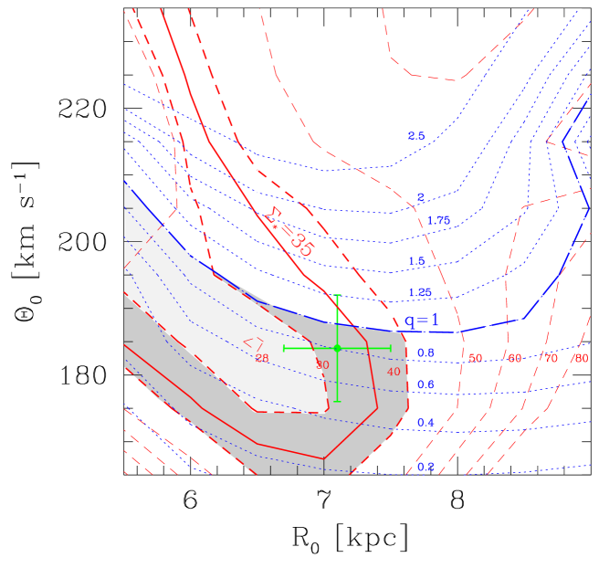
Figure 6: Contours of the stellar column density in the Solar neighbourhood ($\Sigma_{*}$; long dashed lines) and halo flattening ($q$; dotted lines) as a function of the adopted values for the Galactic constants, $R_{0}$ and $\Theta_{0}$. The heavy full line and the heavy dashed line corresponds to Kuijken & Gilmore’s (1989) determination of $\Sigma_{*}$, and the $\pm 1-\sigma$ values. The heavily-shaded region corresponds to parts of parameter space consistent with these values of $\Sigma_{*}$ that produce an oblate halo. The lightly-shaded area gives the corresponding region if we adopt Gould, Bahcall and Flynn’s (1997) values for $\Sigma_{*}$. The cross shows the determination of the Galactic constants based on an analysis of the Oort constants (Olling & Merrifield 1998).

The values obtained for $q$ and $\Sigma_{*}$ for each possible pair of Galactic constants are presented in Fig. 6. Thus, for example, for values of $R_{0}=7.1\,{\rm kpc}$ and $\Theta_{0}=185\,{\rm km}\,{\rm s}^{-1}$, one finds $\Sigma_{*}=35M_{\odot}\,{\rm pc}^{-2}$ and $q=0.7$, corresponding to the intercept that we previously calculated in Fig. 3.

Figure 6 places some interesting limits on the properties of the Milky Way. For example, if we maintain our prejudice that the halo should be oblate ($q<1$), then, unless we adopt a particularly extreme value for $R_{0}$, we find that $\Theta_{0}$ must be less than $\sim 190\,{\rm km}\,{\rm s}^{-1}$. If we also adopt Kuijken & Gilmore’s (1989) measurement of $\Sigma_{*}=35\pm 5M_{\odot}\,{\rm pc}^{-2}$, we find that only models within the heavily-shaded region of Fig. 6 are acceptable, placing an upper limit on $R_{0}$ of $\sim 7.6\,{\rm kpc}$. Conversely, if one forces the Galactic constants to the IAU standard values of $R_{0}=8.5\,{\rm kpc}$ and $\Theta_{0}=220\,{\rm km}\,{\rm s}^{-1}$ (Kerr & Lynden-Bell 1987), one finds barely-credible values of $\Sigma_{*}\sim 60M_{\odot}\,{\rm pc}^{-2}$ and $q\sim 1.5$.

7 Conclusions

The prime objective of this paper has been to check the validity of techniques for measuring halo flattening by asking whether two different techniques return consistent values when applied to the Milky Way. As we have seen in the last section, the answer is a qualified “yes.” The qualification is that consistency with the measured stellar column density requires values of the Galactic constants that differ from those conventionally adopted. However, as was discussed in Section 2, the true values of these constants remain elusive, with estimates spanning the ranges $7\,{\rm kpc}<R_{0}<8.5\,{\rm kpc}$ and $185\,{\rm km}\,{\rm s}^{-1}<\Theta_{0}<235\,{\rm km}\,{\rm s}^{-1}$. With such gross uncertainties, it quite straightforward to pick values that produce an entirely self-consistent picture. To underline this point, we have included on Fig. 6 the results of Olling & Merrifield’s (1997) estimates for $R_{0}$ and $\Theta_{0}$ derived from an analysis of the Oort constants. If that analysis is valid, then we have a consistent model for the Milky Way in which the dark halo has a flattening of $q\sim 0.8$.

Ultimately, this analysis will allow us to come to one of two conclusions:

1. If future studies confirm low values for $R_{0}$ and $\Theta_{0}$ similar to those derived by Olling & Merrifield (1997), then the consistency of the two analyses for calculating $q$ imply that the gas layer flaring technique is valid, adding confidence to the previous determinations by this method.

2. Conversely, if we learn in future that $R_{0}$ and $\Theta_{0}$ are closer to the more conventional larger values, then the implied values of $\Sigma_{*}$ are so far from the observed estimates that one has to suspect that at least one of the techniques for measuring $q$ is compromised. In this case, one would have to look more closely at some of the assumptions that went into the analysis. For example, perhaps the non-thermal pressure forces from cosmic rays and magnetic fields have a role to play even at large radii in galactic disks. Alternatively, perhaps the Hi layer is not close enough to equilibrium for the hydrostatic analysis to be valid. Finally, our assumption of azimuthal symmetry may be invalid. Strong departures from axisymmetry could mean that our determination of the thickness and column density of the gas is compromised, and that the locally determined values of $\Sigma_{1.1}$ and $\Sigma_{*}$ may not be representative for the Galactocentric radius of the Sun.

Assuming for the moment that the analysis is valid, we have another datum to add to Fig. 1. Since the two previous flaring analyses returned systematically rather small values of $q\sim 0.3$, it is reassuring that the Milky Way seems to indicate a larger value of $\sim 0.8$ – it appears that the low values are simply a coincidence arising from the very small number statistics. This larger value is inconsistent with the very flat halos that are predicted by models in which the dark matter consists of either decaying neutrinos (Sciama 1990) or cold molecular hydrogen (Pfenniger, Combes & Martinet 1994).

With the addition of the Milky Way to the data presented in Fig. 1, the only technique that stands out as giving systematically different values for $q$ is the bending mode analysis of warped gas layers. In this regard, it is notable that simulations cast some doubt on the validity of such analyses. The method assumes that warps are manifestations of persistent bending modes that occur when the flattening of a disk and the surrounding dark halo are misaligned. However, the simulations show that gravitational interactions between a misaligned disk and halo rapidly bring the two back into alignment, effectively suppressing this mechanism (e.g. Dubinski & Kuijken 1995, Nelson & Tremaine 1995, Binney, Jiang & Dutta 1998). The number of measurements is still rather small, but it is at least interesting that if one neglects the warped gas layer results, the remaining data appear entirely consistent with the dotted line in Fig. 1, which shows Dubinski’s (1994) prediction for the distribution of halo shapes that will be produced in a cold dark matter cosmology.

References

- [Arnaboldi et al. 1993] Arnaboldi M., Capaccioli M., Cappellaro E., Held E.V., Sparke L.S., 1993, A&A, 267, 21
- [Bahcall 1984] Bahcall J.N., 1984, ApJ, 276, 169
- [Becquaert, Combes & Viallefond 1997] Becquaert J.F., Combes F., Viallefond F. 1997, A&A, 325, 41
- [Begeman 1989] Begeman K., 1989, A&A, 223, 47
- [p. 614] Binney J.J., Merrifield M.R., 1998, Galactic Astronomy, Princeton University Press
- [Binney, Jiang & Dutta 1998] Binney J.J., Jiang I.G., Dutta S., 1998, MNRAS, 297, 1237
- [Bosma 1981] Bosma A., 1981, AJ, 86, 1825
- [Brand & Blitz 1993] Brand J. & Blitz L., 1993, A&A, 275, 67
- [Braun 1998] Braun R., 1998, in Franco J., Carraminana A., eds, Interstellar Turbulence, Proceedings of the 2nd Guillermo Haro Conference, Cambridge University Press.
- [Braun 1997] Braun R., 1997, ApJ, 484, 637
- [Braun & Walterbos 1992] Braun R., Walterbos R.A.M., 1992, ApJ, 386, 120
- [Bronfman et al. 1988] Bronfman L., Cohen R.S., Alvarez H., May J. & Thaddeus P., 1988, ApJ, 324, 248
- [Broeils 1992] Broeils A., 1992, Ph. D. Thesis, University of Groningen
- [Buote & Canizares 1996, 1998]
- [Buote & Canizares 1996] Buote D.A., Canizares C.R., 1996, ApJ, 468, 184
- [Buote & Canizares 1998] Buote D.A., Canizares C.R., 1998, MNRAS, 298, 811
- [Dehnen & Binney 1998] Dehnen W., Binney J., 1998, MNRAS, 294, 429
- [Diplas & Savage 1991] Diplas A. & Savage D.S., 1991, ApJ, 377, 126
- [Dove & Shull 19944] Dove J.D., Shull J.M., 1994, ApJ, 423, 196
- [Dubinski 1994] Dubinski J., 1994, ApJ, 431, 617
- [Dubinski & Kuijken 1995] Dubinski J., Kuijken K., 1995, ApJ, 442, 492
- [Feast & Whitelock 1997] Feast M., Whitelock P., 1997, MNRAS, 291, 683
- [Ferguson et al. 1996] Ferguson A.M.N., Wyse R.F.G., Gallagher J.S., Hunter D.A., 1996, AJ, 111, 2265
- [Gould, Bahcall & Flynn 1997] Gould A., Bahcall J.N., Flynn C. 1997, ApJ, (GBF97)
- [Hofner & Sparke 1994] Hofner P. & Sparke L., 1994, ApJ, 428, 466
- [Katz & Gunn 1991] Katz N., Gunn J.E., 1991, ApJ, 377, 365
- [Kent 1987] Kent S.M., 1987, AJ, 93, 816
- [Kent, Dame & Fazio 1991] Kent S.M., Dame T.M. & Fazio G., 1991, ApJ, 378, 131
- [Kerr & Lynden-Bell 1986] Kerr F.J., Lynden-Bell D., 1986, MNRAS, 221, 1023
- [Kuijken & Gilmore 1991; henceforth KG91]
- [Kuijken & Gilmore 1991] Kuijken K. & Gilmore G., 1991, ApJl, 367, L9 (KG91)
- [Kuijken & Gilmore 1989] Kuijken K. & Gilmore G., 1989b, MNRAS, 239, 605
- [Lake & Feinswog 1989] Lake G., Feinswog L., 1989, AJ, 98, 166
- [Layden et al. 1996] Layden A.C., Hanson R.B., Hawley S.L., Klemola A.R., Hanley C.J., 1996, AJ, 112, 2110
- [Malhotra 1995] Malhotra S., 1995, ApJ, 448, 138
- [Malhotra 1994] Malhotra S., 1994, ApJ, 443, 687
- [Maloney 1993] Maloney P., 1993, ApJ, 414, 41
- [Merrifield 1992] Merrifield M.R., 1992, AJ, 103, 1552
- [Nelson & Tremaine 1995] Nelson R.W., Tremaine S., 1995, MNRAS, 275, 897
- [Olling & Merrifield 1998] Olling R.P., Merrifield M.R., 1998, MNRAS, 295, 737
- [Olling 1996b] Olling R.P., 1996b, AJ, 112, 481-490
- [Olling 1996c] Olling R.P., 1996c, AJ, 112, 457-480
- [Olling 1995] Olling R.P., 1995, AJ, 110, 591
- [Peebles 1993] Peebles P.J.E., 1993, “Principals of Physical Cosmology”, Princeton University Press
- [Pfenniger, Combes & Martinet 1994] Pfenniger D., Combes F., & Martinet L., 1994, A&A, 285, 79
- [Reid etal 1999] Reid M.J., Readhead A.C.S., Vermeulen R.C., Treuhaft R.N., 1999, astro-ph/9905075
- [Reid 1993] Reid M.J., 1993, ARA&A, 31, 345
- [e.g., Rubin, Ford & Thonnard 1980] Rubin V.C., Ford W.K., Thonnard N., 1980, ApJ, 238, 471
- [Sackett 1997] Sackett P.D., 1997, ApJ, 483, 103
- [Sackett & Pogge 1995] Sackett P.D. & Pogge R.W. in Dark Matter, edited by S.S. Holt, C.L. Bennet (AIP conference proceedings 336), 1995, p. 141
- [Sackett et al. 1994] Sackett P.D., Rix H.W., Jarvis B.J. & Freeman K.C., 1994, ApJ, 436, 629
- [Sciama 1990] Sciama D., 1990, MNRAS, 244, 1
- [Steiman-Cameron, Kormendy & Durisen 1992] Steiman-Cameron T.Y., Kormendy J. & Durisen R.H., 1992, AJ, 104, 1339
- [Udry & Martinet 1994] Udry S. & Martinet L., 1994, A&A, 281, 314
- [van Albada & Sancisi 1986] Albada T.S. van & Sancisi R., 1986, Phil. Trans. R. Soc. Lond. A., 320, 447
- [e.g. van Albada & Sancisi 1986]
- [Wang, Heckman & Lehneert 1997] Wang J., Heckman T.M., Lehnert M.D., 1997, ApJ, 491, 114
- [Warren et al. 1992] Warren M.S., Quinn P.J., Salmon J.K., Zurek W.H., 1992, ApJ, 399, 405
- [Wolfire et al. 1995] Wolfire M.G., Hollenbach D., McKee C.F., Tielens A.G.G.M., Bakes E.L.O., 1995, ApJ, 443, 152
- [Wouterloot et al. 1990] Wouterloot J.G.A., Brand J., Burton W.B. & Kwee K.K., 1990, A&A, 230, 21