First Constraints on Iron Abundance versus Reflection Fraction from the Seyfert 1 Galaxy MCG–6-30-15

Abstract

We report on a joint ASCA and RXTE observation spanning an $\sim$ 400 ks time interval of the bright Seyfert 1 galaxy MCG–6-30-15. The data clearly confirm the presence of a broad skewed iron line ($W_{K\alpha}\sim$ 266 eV) and Compton reflection continuum at higher energies reported in our previous paper. We also investigate whether the gravitational and Doppler effects that affect the iron line may also be manifest in the reflected continuum. The uniqueness of this data set is underlined by the extremely good statistics that we obtain from the approximately four million photons that make up the 2-20 keV RXTE PCA spectrum alone. This, coupled with the high energy coverage of HEXTE and the spectral resolution of ASCA in the iron line regime has allowed us to constrain the relationship between abundance and reflection fraction for the first time at the 99 per cent confidence level. The reflection fraction is entirely consistent with a flat disk, i.e. the cold material subtends $\rm 2\pi$ sr at the source, to an accuracy of 20 per cent. Monte Carlo simulations show that the observed strong iron line intensity is explained by an overabundance of iron by a factor of $\sim$ 2 and an underabundance of the lower-Z elements by a similar factor. By considering non-standard abundances, a clear and consistent picture can be made in which both the iron line and reflection continuum come from the same material such as e.g. an accretion disk.

1 INTRODUCTION

The current paradigm for active galactic nuclei (AGN) is a central engine consisting of an accretion disk surrounding a supermassive black hole (e.g. see review by Rees 1984). The main source of energy is gravitational potential energy as material falls in and is heated to high temperatures in some sort of dissipative disk.

The accretion disk is assumed to consist of cold optically thick material. Cold in this context means that iron is more neutral than Fe XVII (oxygen is not fully ionized although H and He may be ionized). Depending on the geometry, this material may be subjected to irradiation. Careful study of the X-ray reprocessing mechanisms can give much information about the immediate environment of the accreting black hole. These effects of reprocessing can often be observed in the form of emission and absorption features in the X-ray spectra of AGNs. In Seyfert 1 nuclei, approximately half of the X-rays are ‘reflected’ off the inner regions of the accretion disk (Guilbert & Rees 1988; Lightman & White 1988), and superposed on the direct (power-law) primary X-ray emission. The general consensus is that the power-law component is emitted in the corona above the disk. As photons pass through the corona, some fraction will be upscattered to X-ray energies. Multiple Compton scatterings tend to produce a power-law X-ray spectrum. The principle observables of the reflection spectrum are a fluorescent iron K$\alpha$ line, and Compton backscattered continuum which hardens the observed spectrum above $\sim$ 10 keV.

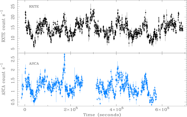
Figure 1: Background-subtracted light curve of MCG$-$6-30-15 for observations in the RXTE PCA 2–60 keV band, and the ASCA SIS 0.5-10 keV band. The epoch of the start and stop times for RXTE and ASCA respectively is 1997 August 4 to 1997 August 12, and 1997 August3 to 1997 August 10.

The iron line together with the reflection component are important diagnostics of the X-ray continuum source. The strength of the emission line relative to the reflection hump between 20–30 keV is largely dependent on the abundance of iron relative to hydrogen in the disk (George & Fabian 1991; hereafter GF91), as well as the normalization of the reflection spectrum relative to the direct spectrum. The relative normalization of the reflection spectrum probably depends primarily on the geometry (i.e. the solid angle subtended by the reflection parts of the disk as seen by the X-ray source). However, strong light bending effects (e.g. Martocchia & Matt 1996) or special-relativistic beaming effects (e.g. Reynolds & Fabian 1997, Beloborodov 1999) can also enhance the amount of reflection.

MCG–6-30-15 is a bright nearby ($z=0.0078$) Seyfert 1 galaxy that has been extensively studied by every major X-ray observatory since its identification. An extended EXOSAT observation provided the first evidence for fluorescent iron line emission (Nandra et al. 1989) which was attributed to X-ray reflection. Confirmation of these iron features by Ginga as well as the discovery of the associated Compton reflected continuum supported the reflection picture (Nandra, Pounds & Stewart 1990; Pounds et al. 1990; Matsuoka et al. 1990) while ASCA data have shown the iron line to be broad, skewed, and variable (eg. Tanaka et al 1995; Iwasawa et al. 1997). The high energy and broad-band coverage afforded by the Rossi X-ray Timing Explorer (RXTE) show convincingly the simultaneous presence of both the broad iron line and reflection component for the first time in this object (Lee et al. 1998). Data on MCG–6-30-15 from BeppoSAX also confirm the presence of a broad skewed iron line and reflection continuum (Guainazzi et al. 1998).

We present in this paper a long look at MCG–6-30-15 simultaneously by RXTE and ASCA spanning a time interval of $\rm\sim 400~{}ks$. (The RXTE on-source time was $\sim$ 400 ks and ASCA on-source time was $\rm\sim 200~{}ks$). Our observations clearly confirm the presence of a redshifted broad iron K$\alpha$ line at $\sim$ 6.3 keV and reflection hump between 20–30 keV. The high energy instrument HEXTE on RXTE coupled with ASCA’s sensitivity at the lower energies allow us to constrain for the first time the relationship between reflection fraction and abundance values at the 99 per cent confidence level. We explore these features of reflection and iron emission in detail. An in-depth investigation of variability is beyond the scope of this paper and will be addressed in a later paper.

2 Observations

MCG–6-30-15 was observed by RXTE spanning $\sim$ 400 ks over the period from 4 Aug 1997 to 12 Aug 1997 by both the Proportional Counter Array (PCA) and High-Energy X-ray Timing Experiment (HEXTE) instruments. (The final useable integration times were 304 ks for the PCA and 114 ks for HEXTE.) It was simultaneously observed for $\rm\sim 200~{}ks$ (with useable intergration time of 197 ks) by the ASCA Solid-state Imaging Spectrometers (SIS) over the period 1997 August 3 to 1997 August 10 with a half-day gap part-way through the observation (PI : H. Inoue). The SIS was operated in Faint mode throughout the observation, using the standard CCD chips (S0C1 and S1C3). We concentrate primarily on the RXTE spectra in this paper.

2.1 RXTE and ASCA Instruments

The Rossi X-Ray Timing Explorer (RXTE) consists of three instruments. The two pointed instruments are the Proportional Counter Array (PCA) that covers the lower energy range and the High Energy X-ray Timing Experiment (HEXTE) that covers the higher energies. Together, the two instruments cover the energy band between 2 and 200 keV. The PCA consists of 5 Xenon Proportional Counter Units (PCUs) sensitive to X-ray energies between 2–60 keV with $\sim 18$ per cent energy resolution at 6 keV. The total collecting area is 6500 $\rm cm^{2}$ ($\sim$ 3900 $\rm cm^{2}$ for 3 PCUs) with a $1^{\circ}$ FWHM field of view. The HEXTE instrument is coaligned with the PCA and covers an energy range between 20–200 keV. For a more thorough review on these instruments, we refer the reader to Jahoda et al. (1996) and Rothschild et al. (1998).

The Advanced Satellite for Cosmology and Astrophysics (ASCA) is a Japanese X-ray observatory that was launched on 1993 February 20, designed and constructed as a joint endeavor with the United States. It consists of four identical grazing-incidence X-ray telescopes, each terminating with a fixed detector. The focal plane detectors are two CCD cameras (Solid state Imaging Spectrometer, or SIS) and two gas scintillation imaging proportional counters (Gas Imaging Spectrometer, or GIS). All four detectors are operated simultaneously all the time. The ASCA SIS is sensitive in the energy range between 0.4 and 10 keV, with an energy resolution of 2 per cent at 5.9 keV. Its field of view is 22 $\rm arcmin^{2}$. The primary goal of the SIS is spectroscopy in the 0.4-10 keV energy band. Its PSF is completely determined by the telescope rather than the detector response. For a more in-depth discussion, we defer to Tanaka, Inoue & Holt (1994).

2.2 Data Analysis

2.2.1 RXTE Reduction

We extract PCA light curves and spectra from only the top Xenon layer using the newly released Ftools 4.1 software. Data from PCUs 0, 1, and 2 are combined to improve signal-to-noise at the expense of slightly blurring the spectral resolution. Data from the remaining PCUs (PCU 3 and 4) are excluded because these instruments are known to periodically suffer discharge and are hence sometimes turned off.

Good time intervals were selected to exclude any earth or South Atlantic Anomaly (SAA) passage occulations, and to ensure stable pointing. We also filter out electron contamination events.

We generate background data using pcabackest v2.0c in order to estimate the internal background caused by interactions between the radiation/particles and the detector/spacecraft at the time of observation. This is done by matching the conditions of observations with those in various model files. The model files used are the L7-240 background models which are intended to be specialized for application to faint sources with count rate less than 100 cts/sec.

The PCA response matrix for the RXTE data set was created using pcarsp v2.36. In the course of performing the spectral fitting described in this section, we discovered a bug in the pcarmf package. This resulted in the 1998-Aug-29 memo (http://legacy.gsfc.nasa.gov/docs/xte/whatsnew/calibration.html#c als41b) from NASA-GSFC detailing the circumstances under which pcarmf does not properly account for the temporal changes in the response matrices. All spectral fitting presented here has been corrected for this software bug. Background models and response matrices are representative of the most up-to-date PCA calibrations.

The net HEXTE spectra were generated by subtracting spectra of the off-source positions from the on-source data. Time intervals were chosen to exclude 32 seconds prior to and 320 seconds following SAA passages. This conservative approach avoids periods when the internal background is changing rapidly. Data in which the satellite elevation is less than 10 degrees above the Earth’s limb is also excluded. We use the standard 1997 March 20 HEXTE response matrices provided by the RXTE Guest Observer Facility (GOF) at Goddard Space Flight Center. The relative normalizations of the PCA and the two HEXTE clusters are allowed to vary, due to uncertainties ( $<$ about 5% ) in the HEXTE deadtime measurement.

2.2.2 ASCA Reduction

ASCA data reduction was carried out using FTOOLS version 4.0 and 4.1 with standard calibration provided by the ASCA GOF. Detected SIS events with a grade of 0, 2, 3 or 4 are used for the analysis. One of the standard data selection criteria, br earth, elevation angle of the source from the bright Earth rim, does not materially affect the hard ASCA data while it does contribute to the soft X-ray data from the SIS at some level. We use the SIS data of approximately 231 ks from each detector for spectral analysis. The source counts are collected from a region centred at the X-ray peak within $\approx$ 4 arcmin from the SIS and 5 arcmin from the GIS. The background data are taken from a (nearly) source-free region in the same detector with the same observing time.

Detection Statistics
Instrument	$\rm{}^{a}EnergyBand$	$\rm{}^{b}CountRate$	$\rm{}^{c}Flux$
ASCA S0 / S1	0.6-10	1.16 / 0.93	-
”	0.5-2	-	1.47
”	2-10	-	3.41
RXTE PCA	2-10	-	4.92
RXTE PCA	3-20	12.72	6.26
HEXTE ClsA / ClsB	16-200	0.73 / 0.63
HEXTE ClsA / ClsB	16-50	-	2.7 / 2.9

Table 1: ^a Energy Band in units of keV. ^b Average count rate for given energy band in units of ct/s. ^c Flux in given energy band in units of $10^{-11}$ ${\rm\thinspace erg}{\rm\thinspace cm}^{-2}{\rm\thinspace s}^{-1}\,$

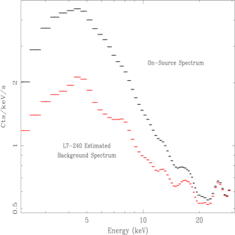
Figure 2: Plot of on-source and estimated background spectra in the energy range 2 keV $<$ E $<$ 30 keV. The background model used is L7-240 appropriate for faint sources and high voltage epoch3.

Table 1 details the average count rate and fluxes for specified energy bands as detected by the ASCA S0 and S1 instruments, and the RXTE PCA and HEXTE Cluster A and Cluster B detectors.

Fig. 1 shows the ASCA S0 160-2700 pha-channel ($\approx$ 0.6–10 keV), and the RXTE PCA 1–129 pha channel ($\approx$ 2-60 keV) background subtracted light curves. There is a gap of $\sim$ 60 ks in the ASCA light curve in which the satellite observed IC4329A while MCG–6-30-15 underwent a large flare observed by RXTE. Significant variability can be seen in both light curves on short and long timescales, which will be investigated in detail in a later paper. Flare and minima events are seen to correlate temporally in both light curves.

3 Spectral Fitting

We fit the data in a number of ways in order to investigate the known features of fluorescent iron emission (eg. Fabian et al. 1994, Tanaka et al. 1995) and Compton reflection (eg. Lee et al. 1998; Pounds et. al. 1990, Matsuoka et al. 1990; Nandra & Pounds 1994) in this object.

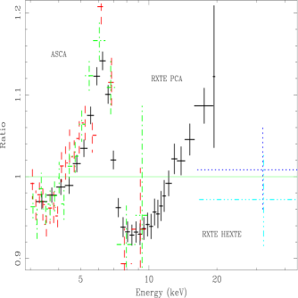
Figure 3: Ratio of data to continuum using a nominal simple power-law fit confirms the clear existence of a redshifted broad iron line at $\sim$ 6.3 keV and reflection component above 10 keV. The simultaneous RXTE and ASCA fit demonstrates the good agreement between the two satellites in the energy band below 10 keV.

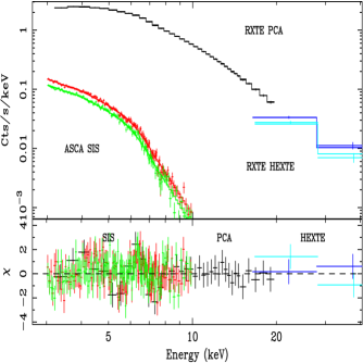
Figure 4: Joint ASCA/PCA/HEXTE spectrum of the simultaneous data from MCG–6-30-15 provide further evidence for the existence of the reflection component and good agreement between ASCA and RXTE. A multicomponent model fit to all three data sets that include a Gaussian component to model the iron line and a reflected spectrum shows that the residuals are essentially flat.

We restrict ASCA and PCA data analysis to be respectively between 3 and 10 keV, and 3 and 20 keV (Fig. 2 shows that the PCA background dominates above 25 keV). This lower energy restriction at 3 keV is selected in order that the necessity for modeling photoelectric absorption due to Galactic ISM material, or the warm absorber that is known to be present in this object is removed. This also allows us to bypass recent problems with residual dark currents in the ASCA 0.5–0.8 keV energy band, and RXTE calibration problems that may still exist at energies below 2 keV. Despite the fact that these absorption features are only important below $\sim$ 2 keV, we nevertheless check their significance in two ways : (1) we fix the column density at the value of $\rm 4.09$ $\rm\times$ $\rm 10^{20}$ $\rm{cm}^{-2}$ to account for Galactic ISM absorption along the line of sight for this object, and (2) we allow this parameter to be free. For both cases, we find that the difference in best fit values between a model that includes and one that excludes this absorption effect is negligible. Additionally, for the latter case we find that the model is unable to place any tight constraints on the column density in the chosen energy range for the RXTE data. Accordingly, we neglect this parameter from our fits. We have also checked that the standard background-subtraction methods described in Section 2.2.1 should adequately account for the PCA background in the energies of interest. As added checks for the quality of the reduction and background subtraction, we extract spectra from 81 ks of Earth-occulted data (elv $\leq$ 0), and find for the occulation data that the normalized flux per keV is zero for the selected energy range. HEXTE data are restricted to be between 16 and 40 keV in order that we may adequately model the reflection hump. HEXTE response matrices are inadequate below 16 keV (William Heindl, 1998 private communication); 0.5 per cent systematics were added to PCA spectra.

3.1 Spectral Features

A nominal fit to all three data sets (i.e. ASCA, RXTE PCA and HEXTE) demonstrates the clear existence of a redshifted broad iron K$\alpha$ line at $\sim$ 6.3 keV and reflection hump between 20 and 30 keV as shown in Lee et al. 1998. Fig. 3 further demonstrates the good agreement between ASCA and RXTE at energies below 10 keV, and in particular, at the energies surrounding the iron line.

As added assurance for the existence of the reflection component and good agreement between ASCA and RXTE, a multicomponent model fit that includes the reflected spectrum to all three data sets shows that the residuals are essentially flat (fig. 4); a gaussian component is used to account for the iron line. The underlying continuum is fit with the model pexrav which is a power law with an exponential cut off at high energies reflected by an optically thick slab of neutral material [Magdziarz & Zdziarski 1995]. We fix the inclination angle of the reflector at $30^{\circ}$ so as to agree with the disk inclination one obtains when fitting accretion disk models to the iron line profile as seen by ASCA (Tanaka et al. 1995). The high energy cutoff is fixed at 100 keV consistent with thermal corona models. We perform fits in which the high energy cutoff is allowed to be a free parameter and find that RXTE is incapable of placing any contraints on this value for MCG–6-30-15 (the best fit values can vary anywhere from $\sim$ 30 keV to a few hundred keV). For this reason, we rely on the values determined by BeppoSAX. (The Phoswitch Detector System PDS on board BeppoSAX has a better spectral sensitivity than the RXTE HEXTE at the higher energies.) For robustness, we further test the sensitivity of RXTE to the high energy cutoff by performing fits in which this parameter is allowed to vary within the 100–400 keV 90% confidence region as determined by BeppoSAX (Guainazzi et al. 1998). The preferred high energy cutoff is 100 keV with infinity as the upper limit error. We also test for the significance of the high energy cutoff value in the determination of fit parameters; this is done by comparing fit results for 100 keV and 400 keV cutoff energies ; the two results do not differ with any statistical significance. We fit the RXTE data in the 3–40 keV energy range with a multiple component model consisting of a power-law reflection and redshifted Gaussian component. Errors are quoted at the 90 per cent confidence ($\Delta\chi^{2}$ = 2.71, Bevington & Robinson 1994).

The best fit values for the 100 keV cutoff energy case are detailed in Table 2. (A double gaussian fit using the ASCA parameters shows a negligible improvement of $\Delta\chi^{2}$ = 3 for one extra parameter.) For comparison, the best fit values for which this cutoff energy was fixed at 400 keV are : power-law slope $\Gamma$ = $2.07^{+0.06}_{-0.04}$ with a power law flux at 1 keV $A=(1.95^{+0.13}_{-0.10})\times 10^{-2}$ $\rm ph$ $\rm cm^{-2}$ $\rm s^{-1}$. The reflection fraction is $0.81^{+0.16}_{-0.15}$ for lower elemental abundances set equal to that of iron of $0.72^{+0.26}_{-0.17}$ solar abundances. The redshifted line energy is $\rm 5.98\pm 0.08~{}keV$ with line width $\sigma$ = $\rm 0.58^{+0.11}_{-0.10}~{}keV$ and intensity of the iron line I = $1.62^{+0.26}_{-0.19}\times 10^{-4}$ ${\rm\thinspace ph}{\rm\thinspace cm}^{-2}{\rm\thinspace s}^{-1}\,$. The equivalent width $W_{K\alpha}$ = $\rm 300^{+48}_{-35}~{}eV$ and $\chi^{2}$ is 39 for 47 degrees of freedom. While the fit values between the two cutoff energy scenarios differ by little, it is clear that a high energy cutoff of 100 keV is preferred ($\Delta\chi^{2}\sim 4$ for no additional parameters). Accordingly, the results that follow are based on this fixed value for the high energy cutoff. We note that the $\chi^{2}$ values are likely to be lower than expected due to the tendency of the reduction software to overestimate the errors.

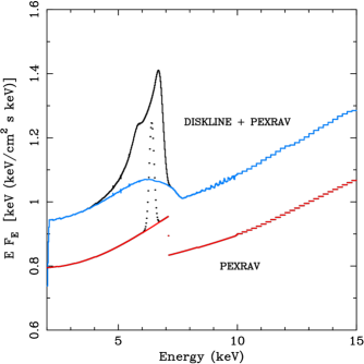
Figure 5: A model that accounts for relativistic smearing of the reflection component with disk-line model parameters (upper plot) as contrasted with a model that does not include Doppler and gravitational effects on the reflected component (lower plot). Note the contrast in the sharpness of the iron edge at $\sim$ 7 keV. The two models have been artificially renormalized for the sake of illustration.

3.2 Doppler and Gravitational effects on the Reflected Spectrum

We next investigate the degree to which gravitational and Doppler effects which determine the line profile also affect the reflection continuum shape (the previous section does not account for this effect). We use a convolution model (rdblur) that assumes the same characteristics as the disk-line model for a Schwarzschild geometry by Fabian et al. (1989) for application to the reflected spectrum. (The reflected continuum is convolved with the same kernel as the diskline model.) For these fits, we assume a cold accretion disk inclined at $i=30^{\circ}$ (Tanaka et al. 1995). The radial emissivity, $\alpha$ assuming a power-law-type emissivity function ($\propto R^{-\alpha}$) of the line, is left as a free parameter. The innermost radius of stable orbit $R_{in}$ for a Schwarzschild geometry is set to Iwasawa et al. (1999) best fit ASCA value $6.7r_{g}$ ; the outermost radius $R_{out}$ is left as a free parameter ($r_{g}\equiv GM/c^{2}$ is the gravitational radius of the black hole), for this object. A comparison between the differences in the two models is shown in fig. 5.

We test for the effects of gravity and Doppler shifts by comparing the quality of the fits using (1) a model that accounts for the effects of relativistically smeared reflection and (2) a model that does not account for this effect. For the latter, the diskline model is used for the iron emission and pexrav for the continuum : pexrav + diskline. A similar model is used for the former with the addition of a multiplicative component (rdblur) that convolves the continuum with the same kernal as the diskline model : rdblur$\ast$(pexrav)+diskline. We have investigated fits in which the lower-Z and iron abundances were tied together and left as free parameters, and fits in which the former was fixed at 0.5 solar abundances and the latter fixed at twice solar abundances appropriate for the $W_{K\alpha}$ value seen in this object. (A more detailed investigation of the effects of abundances on the $W_{K\alpha}$ and reflection fraction is presented in subsequent sections.) The results for the latter (fixed abundances) vacillate between statistically insignificant preferences for relativistically smeared reflection from RXTE data ($\Delta\chi^{2}=1.5$ corresponding to 1 extra ‘hidden’ parameter, for 49 degrees of freedom), and the contrary from ASCA data ($\Delta\chi^{2}=1.5$ for 681 degrees of freedom). We have also searched for this effect in the 1994 ASCA data and find that $\Delta\chi^{2}=0.2$ for 681 degrees of freedom. When the low-Z and iron abundances are untied and left as free parameters, the RXTE data prefer smeared reflection with $\Delta\chi^{2}=2.7$ for 47 degrees of freedom. Additionally, while derivations for the iron abundance remains at twice solar, there is a preference for slightly higher low-Z abundances for the case of smeared reflection. $\Delta\chi^{2}$ values from ASCA remain simliar to those previously mentioned when abundances were fixed; there is a clear indication that ASCA is insensitive to abundance measurements. The reflection fraction is fixed at unity.

While we suspect that relativistic effects are indeed prevalent in the reflected spectrum, it appears that the sensitivity of the present data are insufficient for detecting the effects of relativistically smeared reflection with large statistical significance. We suspect that any deviation in $\chi^{2}$ is largely due to the the modeling of the iron edge at $\rm\sim 7\,keV$ as illustrated in Fig. 5. The contrast is remarkably noticeable at that energy between the models : the standard pexrav model that we use for our fits invokes a sharp edge at those energies which is neither seen in the time-averaged ASCA nor RXTE data. The sharpness and depth of this feature is diminished when we invoke Doppler and gravitational effects. However, we are trying to detect a 10 per cent effect which is also at the level of the ASCA error bars above $\sim$ 7 keV. Differences in $\chi^{2}$ can come additionally from the smearing of the reflection hump, and may be partly the reason that RXTE with its higher energy coverage prefers smeared reflection.

We have checked our findings against the level of present calibration uncertainties in the PCA response matrix. An absorbed power-law and narrow Gaussian fit to a 47 ks archived data of the quasar 3C 273 from the same gain epoch (epoch 3) as our observations give residuals less than 1 per cent for the energies of interest. Furthermore, the best fit 3C 273 values are comparable to those obtained with ASCA and BeppoSAX observations of this object (e.g. Haardt et al. 1998; Orr et al. 1998; Cappi et al. 1998).

However, because fit results from a model that includes the effects of relativistically smeared reflection and one that does not differ by little, we also present results for the former whenever appropriate in this paper. Due to the insensitivity of RXTE to the line profile, the results in which relativistically smeared reflection is considered, presented in Table 2 and subsequently correspond to the model : rdblur$\ast$(pexrav + narrow gaussian) with $\alpha$, $R_{in}$ and $R_{out}$ frozen respectively at 2, $6r_{g}$, and $30r_{g}$ The best fit results are similar to those derived from the diskline models mentioned previously.

3.3 Constraints on Reflection Fraction and Iron Abundance

Having established that the reflection component exists, we next investigate the relationship between the iron abundance and reflection fraction for the reflection scenarios described in sections 3.1 and 3.2. In order to obtain a better understanding of physical models of AGN central regions, we need to disentangle the abundance from the absolute normalization of the reflection component. Due to the lack of good broad spectral coverage in previous observations, the fit parameters of reflection fraction, elemental abundances, and power-law index were strongly coupled. With the high energy coverage of HEXTE and ASCA’s good spectral resolution at energies between 0.6 and 10 keV, we can decouple these parameters for the first time and study the relationship each has with respect to the others. Fig. 6 shows the confidence contours for abundance versus reflection fraction as expected from a corona+disk model. The best fit value for abundance and reflection fraction for the standard pexrav case are respectively $0.92^{+0.31}_{-0.21}$ solar abundances and $1.09^{+0.26}_{-0.19}$; the corresponding values for smeared reflection are $1.13^{+0.31}_{-0.21}$ solar abundances and $1.16^{+0.40}_{-0.26}$. Both results are consistent with the scenario in which the primary X-ray source is above the accretion disk subtending an angle of 2$\pi$ sr (i.e. corresponding to a reflection fraction of $\frac{\Omega}{2\pi}=1$).

Figure 6: Fitting in the energy range 3 keV $\leq$ E $\leq$ 40 keV, we constrain upper bounds for the abundance vs. reflection fraction relationship at the 99 per cent confidence level for the first time. The dot-dashed-line contours correspond to fits in which relativistically smeared reflection (due to Doppler and gravitational effects) is considered; the dotted-line contours do not include this effect. Solid lines represent contours of constant equivalent width; dashed lines correspond to the equivalent width values of $266^{+46}_{-33}$ eV and $331\pm 25$ eV respectively for non-smeared and relativistically smeared reflection.

We wish to stress the uniqueness of this data set for both its good statistics and energy coverage. In the RXTE PCA 2-20 keV spectrum alone, we estimate that $\approx$ 4 million photons make up the spectrum for our 400 ks exposure. (The 2–20 keV flux is $\sim$ 8.6 photons $\rm cm^{-2}\,s^{-1}$ for a detector effective area at those energies of $\rm\sim 1000\,cm^{2}$, for 3 PCUs.) Its uniqueness is underlined by our ability to place combined constraints on both the line and reflection fraction. However, it should be noted that pexrav does not model the iron emission feature which, for the case of RXTE data is achieved using a Gaussian line profile. Accordingly, the consistency of the strength of the line with pexrav predictions for the resulting absorption is investigated via Monte Carlo simulations in the next section. GF91 have shown that the strength of the iron K-shell absorption features can be increased by varying the elemental abundances, or by ionizing the lower atomic weight elements. The enhanced iron abundance causes more iron K-shell absorption of the reflection continuum thereby weakening the reflection continuum as the abundance rises.

For completeness, we also consider the significance of the inclination angle value for our determination of the reflection fraction and abundance results. (We test this only for the non-smeared reflection case since the determination of the inclination is largely due to the iron line peak rather than the reflected continuum.) This test is also relevant for assessing the accuracy of the value we obtain for $W_{K\alpha}$, which is dependent on the inclination and $\Gamma$; ASCA’s determination of the inclination from this observation is $31^{\circ}\pm 2^{\circ}$ (Iwasawa et al. 1999, submitted) consistent with previous observations (Tanaka et al. 1995). For exaggerated inclinations of 20^∘ and 40^∘, we obtain respectively reflection fraction and abundance values to be $1.02^{+0.25}_{-0.18}$ and $0.91^{+0.32}_{-0.21}$, and $1.18^{+0.26}_{-0.21}$ and $0.95^{+0.33}_{-0.22}$ which are within the errors of the values obtained from fits in which we fix the inclination at 30^∘. The apparent insensitivity of RXTE to the inclination value is due to the inability of the satellite to resolve the blue peak of the iron line. The inclination is determined at the energy where the blue peak of the line abruptly drops off; the spectral resolution of RXTE is inadequate for resolving this feature in much detail. $\Gamma$ remains relatively unchanged.

Summary of Spectral Fits for Sections 3.1 – 3.4
Section	$\rm\Gamma_{4-20}^{a}$	$\rm refl^{b}$	$\rm LowZ^{c}$	$\rm Iron^{d}$	$\rm A^{e}$	$\rm LineE^{f}$	$\rm\sigma^{g}$	$\rm I_{K\alpha}^{h}$	$\rm W_{K\alpha}^{i}$	$\rm\chi^{2}/dof^{j}$	$\rm grav^{k}$
3.1	$2.02^{+0.05}_{-0.04}$	$1.09^{+0.26}_{-0.19}$	$0.92^{+0.31}_{-0.21}$	= abund	$1.88^{+0.11}_{-0.09}$	$5.99^{+0.07}_{-0.09}$	$0.54^{+0.11}_{-0.10}$	$1.45^{+0.25}_{-0.18}$	$266^{+46}_{-33}$	35/47
3.2	$1.99\pm 0.04$	$1.13^{+0.31}_{-0.21}$	$1.16^{+0.40}_{-0.26}$	= abund	$1.91^{+0.11}_{-0.09}$	$6.28\pm 0.05$	$0.05^{+0.17}_{-0.05}$	$1.74^{+0.13}_{-0.13}$	$331^{+25}_{-25}$	24/47	$\surd$
3.4	$2.01^{+0.04}_{-0.05}$	1	$0.44^{+0.32}_{-0.11}$	$2.05^{+2.05}_{-0.99}$	$1.80^{+0.10}_{-0.10}$	$5.98\pm 0.08$	${\bf 0.54}$	$1.14^{+0.29}_{-0.33}$	$201^{+51}_{-58}$	31/49
3.4	$1.98\pm 0.04$	1	$0.82^{+1.03}_{-0.38}$	$1.50^{+2.05}_{-1.04}$	$1.88^{+0.11}_{-0.11}$	$6.29^{+0.63}_{-0.57}$	${\bf 0}$	$1.66^{+0.30}_{-0.29}$	$312^{+56}_{-55}$	24/49	$\surd$

Table 2: Summary of fits as discussed in sections 3.1–3.4. Bold-faced values indicate parameters that were fixed at the value given. For all fit values indicated here, the redshift and high energy cutoff were consistently fixed at the values of 0.0078 and 100 keV respectively, with inclination fix at best fit ASCA value of $30^{\circ}$. ^a Power-law photon index. ^b Reflective fraction = $\Omega/2\pi$. ^c Lower elemental abundances relative to solar abundances. ^d Iron abundances relative to solar. ^e Power-law flux at 1 keV, in units of $10^{-2}$ $\rm ph$ $\rm cm^{2}$ $\rm s^{-1}$ $\rm keV^{-1}$. ^f Energy of the iron $K\alpha$. ^g Iron line width (keV) ^h Intensity of iron emission line in units of $10^{-4}$ ${\rm\thinspace ph}{\rm\thinspace cm}^{-2}{\rm\thinspace s}^{-1}\,$. ⁱ Equivalent width of the emission line in units of eV. ^j $\chi^{2}$ per degree of freedom. ^k Column is checked if relativistically smeared reflection is accounted for in the fit.

3.4 Iron Abundance and Strength of the Reflected Continuum

Up until this point, we have treated the iron emission and absorption (which has direct bearing on the derived reflection fraction) as separate additive components of a multi-component model. This is due largely to pexrav modelling only the reflection continuum, which is imprinted with the absorption feature. However, we need to assess the consistency of the line intensity with pexrav model predictions of this absorption. This is now discussed in the context of Monte Carlo simulations.

Previous workers (i.e. GF91; Matt, Perola & Piro 1991; Reynolds, Fabian, & Inoue 1995) have investigated the effect of abundance values on the equivalent width of the line and the associated reflected spectrum. This was done via Monte Carlo simulations in which incident photons are assigned a random initial energy with a power-law distribution function $\Gamma\sim 1.9$, and an incident energy (corresponding to an isotropic source). The probabilities for a photon to be either Compton scattered or photoelectrically absorbed for a given energy are tracked.

The equivalent width of the iron line in MCG–6-30-15 is $\rm 266^{+46}_{-33}~{}eV$ and $\rm 331\pm 25~{}eV$ for non-smeared and smeared reflection respectively, when the reflector has $\sim$ solar abundance and reflection fraction close to unity. Both are inconsistent with the predicted $W_{K\alpha}$ of $\rm 150~{}eV$ from GF91 for a slab of cold material subtending $\rm 2\pi~{}sr$ at the X-ray source, rotating around a static black hole. We show in Fig. 6 the locus of points in the abundance – reflection plane which has an equivalent width of $250\pm 100{\rm\thinspace eV}$. It is clear that the highest reflection fraction part of the diagram leads to a much stronger line than is observed. The best-fitting solution lies within the region defined by the reflection-fitting contours and the lines of observed equivalent width.

Some fraction of an iron line can be due to reflection from outer material (the putative torus say). This fraction is however likely to be small in MCG–6-30-15 since the part of the line consistent with a zero-velocity narrow core sometimes disappears at some phases of the ASCA data (Iwasawa et al 1996).

The equivalent width of the line does not depend however on the iron abundance alone, but also upon the abundance of the lower-Z elements such as oxygen which can absorb the line before it emerges from the reflector. We have therefore investigated the behaviour of the solution in the multi-dimensional, iron abundance, lower-Z abundance, reflection fraction space. To make the problem tractable we adopt unit reflection fraction. This is indeed the preferred solution when the iron and lower-Z abundances are separated. The contours in the abundance plane for the (non-smeared) results are shown in Fig. 7, showing that separate abundances are indeed preferred. We then use a Monte-Carlo code to track the predicted equivalent width along the major locus of the abundance contours. The equivalent widths are shown in Fig. 8 and reveal that a value of 300 eV occurs when the iron abundance is about twice the solar value and the lower-Z abundances are about half the solar value. Details of actual fit values using the pexrav and relativistically smeared reflection models can be found in Table 2.

Figure 7: Confidence contours (corresponding to 68, 90, and 99 per cent confidence levels) for iron abundance versus lower elemental abundances for material subtending 2$\pi$ sr at the X-ray source. The ’+’ symbol correspond to the best fit values ; the ’x’ symbols are used for illustrative purposes for Fig. 8.

Figure 8: Filled hexagons correspond to plot of equivalent width of the fluorescent iron K$\alpha$ line as a function of iron abundance for 30^∘ inclination. The results are based on Monte Carlo simulations in which the low-Z abundances and iron abundance values (as defined by Morrison & McCammon 1983) are modified according to the locus of points illustrated by the symbol ’x’ in the contour plot of Fig. 7. The chosen abundance and iron abundance values used in the simulations are represented by filled triangles.

4 Discussion

This simultaneous long observation coupled with the combined strengths of ASCA and RXTE have enabled us to constrain for the first time the relationship between iron abundance and reflection fraction at the 99 per cent confidence level, as well as confirm the presence of a broad skewed iron line for MCG–6-30-15. With the additional high energy coverage of HEXTE, we establish that the features of reflection are present and that results are consistent with the scenario in which cold material subtends $2\pi$ sr at the X-ray source. We further investigate the effects of gravity and Doppler shifts on the reflection component, but find that both RXTE and ASCA are insensitive to this. Additionally, we verify that the effects of the cutoff energy do not compromise our results. By fitting the data with the 100 keV lower limit for the cutoff energy and comparing that to the 400 keV cutoff energy fit results, we find that they are consistent with each other within their errors. The preferred cutoff energy however is 100 keV.

Monte Carlo simulations further reveal that an overabundance of iron by a factor of $\sim$ 2 is needed to reconcile the large value for the equivalent width that we observe for both the standard and relativistically smeared reflection scenarios; the equivalent width is even more dramatically enhanced when relativistivistic effects are invoked. By considering non-standard abundances, a consistent picture can be made for which both the iron line and reflection continuum originate from the same material / structure such as, e.g. an accretion disk. We find also that the factor of two to three iron overabundance as predicted by our data holds consistently even in comparisons with models of FeII emission, known to strongly contribute to the optical and UV continuum of many active objects (Wills, Netzer, & Wills 1985). It is also note-worthy to consider the importance of abundance determinations for assessing the chemical history of the host galaxy. For example, an iron rich environment with depleted amounts of lighter elements (as suggested in our data) may provide evidence that Type Ia supernovae events were likely to have occurred in high proportions during the history of the galaxy.

5 ACKNOWLEDGEMENTS

We thank all the members of the RXTE GOF for answering our inquiries in such a timely manner, with special thanks to William Heindl and the HEXTE team for help with HEXTE data reduction. We also thank Keith Jahoda for explanations of PCA calibration issues, and Roderick Johnstone and Keith Arnaud for their time and help with software. JCL thanks the Isaac Newton Trust, the Overseas Research Studentship programme (ORS) and the Cambridge Commonwealth Trust for support. ACF thanks the Royal Society for support. WNB thanks the NASA RXTE grant NAG5-6852, and the NASA Long Term Space Astrophysics (LTSA) grant NAG5-8107 for support. CSR thanks the National Science Foundation for support under grant AST9529175, and NASA for support under the LTSA grant NASA-NAG-6337. KI thanks PPARC.

References

- [] Beloborodov A. M., 1999, ApJ., 510L, 123B
- [] Bevington P. R., Robinson D. K., 1994, Data Reduction and Error Analysis for the Physical Sciences Edition 2, McGraw-Hill, New York
- [] Cappi M., Matsuoka M., Otani C., Leighly K. M., 1998, PASJ, 50:213
- [Fabian, et al. 1994] Fabian A. C., et al, 1994, PASJ, 46, L59
- [Fabian, et al. 1989] Fabian A. C., Rees M. J., Stella L., White H. E., 1989, MNRAS, 238, 729
- [George & Fabian 1991] George I. M., Fabian A. C., 1991, MNRAS, 249, 352
- [1] Guainazzi M., Matt G., Molendi S., Orr A., Fiore F., Grandi P., Matteuzzi A., Mineo T., Perola G. C., Parmar A. N., Piro L., 1998, A&A
- [Guilbert & Rees 1988] Guilbert P. W., Rees M. J., 1988, MNRAS, 233, 475
- [] Haardt F., Fossati G., Grandi P., Celotti A., Pian E., Ghisellini G., Malizia A., Marashi L., Paciesas W., Raiteri C. M., Tagliaferri, G., Treves A., Urry C. M., Villata M., Wagner S., 1998, A&Ai, 340, 35
- [Iwasawa, et al. 1997] Iwasawa K., Fabian A. C., Young A. J., Inoue H., Matsumoto C., 1999, MNRAS, submitted
- [Iwasawa, et al. 1997] Iwasawa K., Fabian A. C., Reynolds C. S., Nandra K., Otani C., Inoue H., Hayashida K., Brandt W. N., Dotani T., Kunieda H., Matsuoka M., Tanaka Y., 1997, MNRAS, 282, 1038
- [] Jahoda K., Swank J. H., Giles A. B., Stark M. J., Strohmayer T., Zhang W., Morgan E. H., 1996, in EUV, X-ray, and Gamma-Ray Instrumentation for Astronomy VII, ed. O. H. Siegmund, (Bellingham, WA: SPIE), 59
- [Lightman & White 1988] Lightman A. P., White T. R., 1988, ApJ., 335, 57
- [Lee et al. 1998] Lee J.C., Fabian A. C., Reynolds C. S., Iwasawa K., Brandt W. N., 1998, MNRAS, 300, 583
- [Magdziarz & Zdziarski 1995] Magdziarz P., Zdziarski A., 1995, MNRAS, 273, 837
- [Martocchia and Matt 1996] Martocchia A., Matt G., 1996, MNRAS, 282, L53
- [Matsuoka et al. 1990] Matsuoka M., Yamauchi M., Piro L., Murakami T., 1990, ApJ, 361, 440
- [Matt et al. 1991] Matt G., Perola G. C., Piro L., 1991, A&A, 247, 25
- [Morrison nd McCammon 1983] Morrison R., McCammon D., 1983, ApJ, 270, 119
- [Nandra & Pounds 1994] Nandra K., Pounds K. A., 1994, MNRAS, 268, 405
- [Nandra & Pounds 1989] Nandra K., Pounds K., Stewart G. C., Fabian A. C., Rees M. J., 1989, MNRAS 236, 39p
- [Nandra, Pounds, & Stewart 1990] Nandra K., Pounds K., Stewart G. C., 1990, MNRAS, 242, 660
- [] Orr A., Yaqoob T., Parmar A. N., Piro L, White N. E., Grandi P., 1998, A&A, 337, 685
- [Pounds, et al. 1990] Pounds K. A., Nandra K., Stewart G. C., George I. M., Fabian A. C., 1990, Nat, 344, 132
- [Rees 1984] Rees M. J., 1984, A&AR, 22, 471
- [Reynolds & Fabian 1997] Reynolds C. S., Fabian, A. C., 1997. MNRAS, 290, L1
- [Reynolds, Fabian, & Inoue 1995] Reynolds C. S., Fabian A. C., Inoue H., 1995, MNRAS, 276, 1311
- [Reynolds, et al. 1995] Reynolds C. S., Fabian A. C., Nandra K., Inoue H., Kunieda H., Iwasawa K., 1995, MNRAS, 277 901
- [Reynolds, et al. 1997] Reynolds C. S., Ward qM. J., Fabian A. C., Celotti A., 1997b, MNRAS, 291, 403
- [] Rothschild R. E. et al., 1998, ApJ, 496, 538
- [] Tanaka Y., Inoue H., Holt S. S., 1994, PASJ, 46, L37
- [Tanaka , 1995] Tanaka Y., Nandra K., Fabian A. C., Inoue H., Otani C., Dotani T., Hayashida K., Iwasawa K., Kii T., Kunieda H., Makino F., Matsuoka M., 1995, Nat., 375, 659
- [] Wills B. J., Netzer H., Wills D., 1985, ApJ., 288, 94