The Hubble Deep Fields: North vs. South

Stephen D. J. Gwyn

Abstract

Photometric redshifts have been calculated for the Hubble Deep Fields. The redshift distributions of the fields differ; there is a large excess of galaxies in the HDF-North in the redshift range $0.4<z<1.2$ . The difference is consistent with the presence of a weak cluster in the HDFN and is only slightly larger than the cosmic variance in other fields of similar depths and with models of large scale structure.

Department of Physics and Astronomy, University of Victoria, P.O. Box 3055, Victoria, BC, Canada V8W 3P6

1. Introduction

The Hubble Deep Field North (Williams et al. 1996) resulted in dozens of papers on galaxy evolution. All these papers treat the HDFN as a typical field; the conclusions that are drawn are assumed to hold for all fields. With the advent of the HDF South (Williams et al. 1999) it is possible to test this hypothesis.

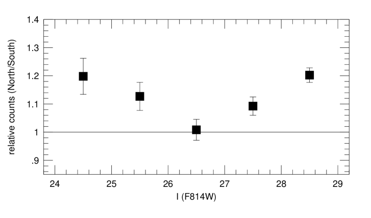
The two fields do show some differences. The number counts of Ferguson (1999, this volume) show a that the HDFN holds 15% more galaxies. This excess is more visible when the differential counts are plotted as shown in Figure 1. Only a fraction of the galaxies in the HDFN and virtually none of the galaxies in the HDFS have spectroscopic redshifts. Thus the question “where do these excess galaxies in the HDFN lie?” must be addressed with photometric redshifts.

Refer to caption — Figure 1.: Relative number counts for the Hubble Deep Fields. The ratio (North divided by South) of the F814W number counts in each magnitude bin is shown. There are roughly 15% more galaxies in the HDFN compared to the HDFS

2. Catalogs and Photometry

The galaxy catalogs and photometry are generated using SExtractor (Bertin & Arnouts, 1996) and additional software written by the author. First, SExtractor is run on the I band image of the HDFN (version 2) and the HDFS (version 1) mosaics. SExtractor does an excellent job of deblending objects. The few errors it makes take the form of splitting single large, bright galaxies into fragments. These are easily corrected by hand.

When determining photometric redshifts, one should measure the colours of galaxies through the smallest feasible aperture. Using a small aperture decreases the random error in the colours, at the expense of introducing systematic shifts if there is a colour gradient in the galaxy. These systematic effects are actually desirable since they generally take form a reddening towards the centre. Since reddening implies an increase in the amplitude of the 4000Å break, it is then easier to determine a photometric redshift. Using small apertures also minimises the chance of contamination by other nearby galaxies. However, it is desirable to construct a catalog using a larger aperture to avoid the systematic errors.

For these reasons, the final catalog contained galaxies with with $I_{ST}<$ 28¹¹1 All magnitudes in this article are given on the ST magnitude system unless otherwise specified. The ST magnitude system is defined such that zero magnitude corresponds to $F_{\lambda}=3.63\times 10^{-12}~{}W\mu^{-1}$ cm^-2 in all band passes. This is similar to the AB system which is defined in terms of a constant value of $F_{\nu}$ but is convenient for comparing magnitudes to template spectra which are usual given in $F_{\lambda}(\lambda)$ . ( $I_{AB}<$ 27.2) as measured through the 1.0 arcsecond aperture. The colours measured through the smaller, 0.5 arcsecond, aperture are used to determine photometric redshifts. In both cases, pixels that lie within the isophotes of other nearby galaxies (as determined using the segmentation image generated by SExtractor) are excluded from the aperture. Because the HDF frames in the different bands are registered to within a fraction of a pixel, the same pixels can be excluded on each frame. This prevents colour contamination which could affect the photometric redshifts. Such contamination has particularly undesirable effects when faint U-band or B-band dropout galaxies lie near bright foreground galaxies.

3. Photometric Redshifts

The galaxies in the the Hubble Deep Fields span a large range in redshifts: The available spectroscopic redshifts in the Hubble Deep Fields, although numerous below $z=1$ and in the range $2<z<3$ , are spotty in the range $1<z<2$ and almost non-existent above $z=3$ . The various linear regression photometric redshift techniques (e.g. Connolly et al., this volume) rely on a training set of spectroscopic redshifts. These techniques, although effective at low redshifts where such a training set exists, are unreliable where the spectroscopic coverage is sparse. Therefore, the photometric redshifts in this article are calculated using the template fitting technique.

The templates are constructed from the observed spectral energy distributions of local galaxies. The four spectra of Coleman, Wu & Weedman (1980, CWW) were used initially. It was found however, that many of the blue galaxies in the Hubble Deep Fields are not well fit by even the bluest CWW spectrum. This caused moderate discrepancies when the photometric redshifts were compared to the spectroscopic redshifts. Therefore the CWW spectra are supplemented with the SB3 and SB2 spectra from Kinney et al. (1996) to form the basis of the template set. From this basis set of six spectra, intermediate templates are constructed by interpolation for a total of 51 templates.

These templates are redshifted at intervals of 0.02 in $\log_{10}(z)$ . Spacing the templates in $\log z$ is an improvement over the more usual linear spacing. It allows, for the same total number of templates, tighter coverage at low redshift (where it is most needed) at the small sacrifice of sparse coverage at high redshift (where it is not needed). The spectra are corrected for intergalactic absorption as prescribed by Madau (1995) After redshifting, the templates are multiplied by the response function of the UBRI filters to produce fluxes at the central wavelength of each filter. These fluxes are converted to magnitudes to form the final templates.

Each template is compared to the observed galaxy magnitudes in turn and a $\chi^{2}$ is determined:

\chi^{2}=\sum_{i=1}^{N_{filters}}{(M_{i}-T_{i}-\alpha)^{2}\over\sigma_{M_{i}}^{2}},

(1)

Where $M_{i}$ is the observed magnitude of the galaxy, $\sigma_{M_{i}}$ is the magnitude uncertainty, $T_{i}$ is the template magnitude, and $\alpha$ is a normalisation factor that corrects the templates to the apparent magnitude of the galaxy. The optimal normalisation factor is determined by minimising equation (1) with respect to $\alpha$ .

In many cases the galaxy is undetected in one or more of the band passes. This can occur when the galaxy when a galaxy is at high redshift and its UV flux has been absorbed by the IGM (the U-band dropouts). However, this can also occur with intrinsically faint, low redshift galaxies. The situation is handled by replacing the relevant term of the sum in equation (1). If the magnitude predicted by template is less than the magnitude limit in that band, the term is replaced with zero. If this isn’t case, on the other hand, the term is replaced with

{M_{\rm limit}-T_{i}-\alpha\over\sigma_{T_{i}}^{2}}

(2)

where $M_{limit}$ is the magnitude limit of the image in question. The weighting factor, $\sigma_{T_{i}}$ , is the uncertainty that the galaxy’s magnitude would have if it was visible in that bandpass.

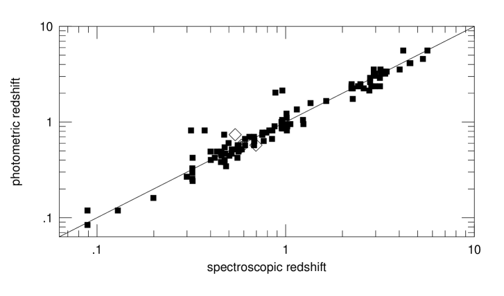
As a check on the accuracy of the technique, photometric redshifts were calculated by the above method for galaxies in both Hubble Deep Fields which have spectroscopic redshifts. The comparison is shown in Figure 2. The redshift uncertainties scale with z. The typical relative error in the photometric redshifts is $\sigma_{z}/z=11\%$ .

4. The Comparison

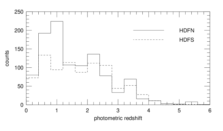
The photometric redshift technique described in section 3 was applied to the photometric catalogs described in section 2. The resulting redshift distributions for the HDF North and South are shown in Figure 3. The two redshift distributions are not the same. The Kolmogorov-Smirnov test gives the probability of the two distributions being the same as $1.2\times 10^{-6}$ . The redshift distributions are most different in the redshift range $0.4<z<1.2$ .

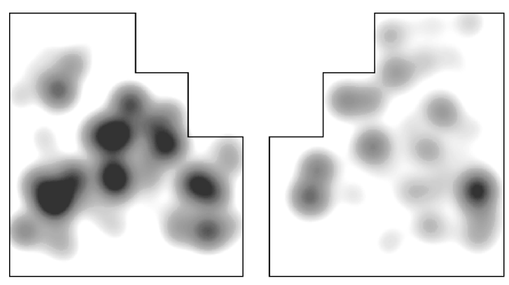
It is tempting to ascribe the differences in the Hubble Deep Fields to a structure present in the North but not in the South. Indeed, there is a pronounced spike in the spectroscopic redshift distribution of the HDFN at $z=0.475$ (Cohen et al. 1996). Figure 4 shows the I band images of the Hubble Deep Fields. Only light from galaxies with photometric redshifts in the range $0.4<z<0.8$ is shown; the other galaxies been masked out. The images have been convolved with Gaussian profile ( $\sigma=6$ arcseconds). The left image shows a large concentration of light in the HDFN that is not present in the South.

The two-point angular correlation function was computed for various redshift slices. Note that it is impracticable to calculate the angular correlation function for slices much narrower than about $\Delta z=.4$ without running into problems with small number statistics. Also, because of the uncertainties on the redshifts, it would be difficult to compute a reliable spatial (as opposed to angular) correlation function. The correlation functions for both fields were compared for each slice. For most redshift slices, they showed no difference within the errors. The only exception was the in the $0.4<z<0.8$ redshift slice, where galaxies in the HDFN were significantly more clustered than in the HDFS. The spatial scale of the structure (the HDF is $\sim$ 1 Mpc across at that redshift) and the number of galaxies involved ( $\sim 50$ more galaxies in the North than in the South) suggest a very poor cluster or a very rich group.

More generally, the differences in the redshift distributions could be due to cosmic variance in the large scale galaxy distribution. This hypothesis was tested empirically in the following manner: The William Herschel Deep Field (WHDF, Metcalfe et al. 1999 in press) extends to $B=28$ and has good coverage in the UBRIHK bands. It covers roughly 40 square arcminutes. The WHDF was divided into 9 separate areas, each the same size as the Hubble Deep Fields. The field to field variance was found to be 10% (rms), smaller than, but not inconsistent with, the difference between the HDFN and HDFS.

N-body simulations computed by Stadel (private communication) indicate the variance in the mass distribution along lines of sight comparable the HDF are about 20% out to $z=1$ . Assuming that galaxies are linearly biased (Kauffman, 1998), this should translate into a similar variance in the redshift distributions in the Hubble Deep Fields. Again this is slightly smaller than, not but not inconsistent with, the difference between the two redshift distributions below $z=1$ as seen in Figure 3.

References

Bertin, E., & Arnouts, S. 1996, A&A, 117, 393

Cohen, J. G., Cowie, L. L., Hogg, D. W., Songaila, A., Blandford, R., & Hu, E. M. 1996, ApJ, 471, L5

Coleman, G. D., Wu C-C. & Weedman, D. W. 1980, 43, 393 (CWW)

Kauffmann, G., Colberg, J. M., Diaferio, A., White, S. D. M. 1998, astro-ph/98091678

Kinney, A. L., Calzetti, D., Bohlin, R. C., McQuade K., Storchi-Bergmann, T., & Schmidt, H. R. 1996, ApJ, 467 38

Madau, P. 1995, ApJ, 441, 18

Williams, R. E. et al. 1996, AJ, 112, 1335

Williams, R. E. et al. 1999, in preparation