Fast rotation of strange stars

Abstract

Exact models of uniformly rotating strange stars, built of self bound quark matter, are calculated within the framework of general relativity. This is made possible thanks to a new numerical technique capable to handle the strong density discontinuity at the surface of these stars. Numerical calculations are done for a simple MIT bag model equation of state of strange quark matter. Evolutionary sequences of models of rotating strange stars at constant baryon mass are calculated. Maximally rotating configurations of strange stars are determined, assuming that the rotation frequency is limited by the mass shedding and the secular instability with respect to axisymmetric perturbarions. Exact formulae which give the dependence of the maximum rotation frequency, and of the maximum mass and corresponding radius of rotating configurations, on the value of the bag constant, are obtained. The values of $T/W$ for rapidly rotating massive strange stars are significantly higher than those for ordinary neutron stars. This might indicate particular susceptibility of rapidly rotating strange stars to triaxial instabilities.

1 Introduction

A deconfined, beta stable quark matter is composed of the u, d, and s quarks, and in contrast to “ordinary” baryon matter has the strangeness per unit baryon number $\simeq-1$ (therefore the name ‘strange quark matter’). An intriguing possibility that such strange matter could be the absolute ground state of matter at zero pressure and temparature was pointed out in an influential paper of Witten (1984) [such a possibility has been contemplated before by Bodmer (1971)]. This possibility is not excluded by what we know from laboratory nuclear physics. If the hypothesis of strange matter is true, then some of neutron stars could be actually strange stars, built entirely of strange matter (Haensel et al. 1986, Alcock et al. 1986; arguments against the existence of strange stars have been presented by Alpar (1987), and Caldwell & Friedman (1991) ).

Detailed models of nonrotating strange stars were constructed in (Haensel et al. 1986, Alcock et al. 1986). Calculations concerning physics and astrophysics of strange stars, published up to 1991, were reviewed in (Madsen & Haensel 1991). References to more recent work on strange stars can be found in review articles by Weber et al. (1995) and Madsen (1999), and in the monograph of Glendenning (1997). Most recently, strange stars have been invoked in models of X-ray bursters (Bombaci 1997, Cheng et al. 1998) and of gamma-ray bursters (Dai & Lu 1998).

Rapid rotation of strange stars has become a topic of interest in 1989, after a sensational (but subsequently withdrawn) claim of detection of a $0.5$ ms pulsar in SN 1987A. In several papers, strange star has been advanced as an appropriate model for a half-millisecond pulsar (Glendenning 1989a,b, Frieman & Olinto 1989). However, several authors pointed out that the experimental constraints on the strange matter model imply that strange stars could not rotate so fast (Haensel and Zdunik 1989, Lattimer et al. 1990, Zdunik & Haensel 1990, Prakash et al. 1990). Subsequent studies of rapid rotation of strange stars focused on the effect of rotation on the structure of the normal crust (Glendenning & Weber 1992).

Recently, it has been shown that fast rotation of hot, young neutron stars is severely limited by the emission of gravitational radiation, due to r-mode instability [for a review, see e.g. Stergioulas (1998)]. However, in contrast to newly born neutron stars, hot strange stars are not subject to the r-mode instability (Madsen 1998). Therefore, strange stars formed in collapse of rotating stellar cores can rotate very fast. This gives additional motivation for studying rapid rotation of strange stars.

It should be stressed, that nearly all calculations of uniformly rotating models of strange stars were done within the slow rotation approximation (see, e.g., Colpi & Miller 1992, Glendenning & Weber 1992). Actually, in the calculations of Glendenning & Weber (1992) the slow rotation scheme, pioneered by Hartle (1967, 1973) and Hartle & Thorne (1968), was supplemented by a “self-consistency condition” at the Keplerian frequency (Weber & Glendenning 1991, 1992). However, the slow rotation approximation is not valid near the shedding (Keplerian) limit. As discussed by Salgado et al. (1994a, b), the improved, “self-consistent” version of this approximation, overestimates by more than 10% the maximum rotation frequency of neutron star models.

So far, the only exact calculations of the rapidly rotating models of strange stars were done by Friedman (quoted in Glendenning 1989a,b) and Lattimer et al. (1990). However, the precision of their numerical results, calculated for one specific equation of state of strange matter, was not checked using an independent exact calculation. Also, the fact that their 2-D code was based on the Butterworth & Ipser (1976) scheme, rises some suspicion concerning its precision when applied to the equation of state of strange matter, characterized by huge density discontinuity at the stellar surface. Indeed Butterworth & Ipser (1976) considered the case of a density discontinuity at the stellar surface – they computed configurations of rotating homogeneous bodies, but as we discuss below (Sec. 4.3), they treated properly the discontinuity only in the radial direction, which is not sufficient for objects which deviate substancially from the spherical symmetry.

In the present paper we perform exact calculations of rapidly rotating strange stars, composed entirely of strange quark matter. Our calculations are based on a multi-domain spectral method recently developed by Bonazzola et al. (1998b). Such a multi-domain technique enables us to treat exactly the density discontinuity at the surface of strange stars. The calculations are performed for a family of equations of state of strange quark matter. On one hand, precision of our calculation is checked using internal error estimators. On the other hand, the validity of scaling relations for the rotating configurations, displayed by our numerical results, yields an additional test of precision of our calculations. Finally, we address the problem of triaxial instabilities of rapidly rotating strange stars, and point out differences with respect to normal neutron stars.

In Sect. 2 we discuss the equation of state of strange matter, based on the MIT bag model of quark matter. The set of equations to be solved and the numerical procedure is presented in Sect. 3. Stationary, uniformly rotating configuration of strange stars are studied in Sect. 4, where we also derive exact scaling relations for the parameters of the rotating strange star models. Parameters of the maximally rotating configurations, stable with respect to the axially-symmetric perturbations, are calculated in Sect. 5, and an exact formula for the maximum rotation frequency of rotating strange stars is derived. We derive also exact formulae for mass and radius of the maximum mass configuration of rotating strange stars. In Sect. 6, we study the problem of triaxial instabilities of rapidly rotating strange stars, and show, that rapidly rotating strange stars might be more susceptible to these instabilities than ordinary neutron stars. Finally, Sect. 7 contains a discussion of our results and the conclusion.

2 Equation of state and static models of bare strange stars

Equation of state of strange matter will be based on the MIT bag model. Baryon number density of strange matter is $n={1\over 3}(n_{\rm u}+n_{\rm d}+n_{\rm s})$, where $n_{\rm u}$ is the number density of the u-quarks etc. In what follows, we will use the simplest model of self-bound strange quark matter, ignoring the strange quark mass and neglecting the quark interactions except for the confinement effects described by the bag constant. We consider thus massless, noninteracting u, d, s quarks, confined to the bag volume. In the case of a bare strange star, the boundary of the bag coincides with stellar surface.

Using the model described above, one can express the energy density, $\epsilon$, and the pressure, $P$, of strange quark matter, as functions of the baryon number density, $n$, in the following form

$$\epsilon = an^{4\over 3}+B\leavevmode\nobreak\ ,$$

$$P = {1\over 3}an^{4\over 3}-B\leavevmode\nobreak\ ,$$ (1)

where $B$ is the MIT bag constant, and the parameter $a$ is given by

$$a={9\over 4}\pi^{2\over 3}\hbar c=952.371\leavevmode\nobreak\ {\rm MeV\leavevmode\nobreak\ fm}\ .$$ (2)

The bag constant $B$ describes the difference in the energy density of the true (real) vacuum and that of the QCD vacuum. This parameter plays a crucial role in the MIT bag model, being actually responsible for the quark confinement. Let us mention, that in the case of a bare strange star of $\sim{\rm M_{\odot}}$ we are dealing with a bag of a radius of $\sim 10\leavevmode\nobreak\ {\rm km}$, containing $\sim 10^{57}$ quarks.

Figure 1: Adiabatic index of strange quark matter, $\gamma$, versus baryon density, $n$. Two vertical dashed lines correspond to strange star surface (left line), and maximum density within static strange star models (right line). Horizontal dashed line corresponds to $\gamma=4/3$, characteristic of free ultrarelativistic Fermi gas.

The constant $B$ represents a natural unit for both the energy density and the pressure. Defining dimensionless energy density and pressure of strange matter, $\widetilde{\epsilon}\equiv\epsilon/B$, $\widetilde{P}=P/B$, we can write down a dimensionless form of the EOS of strange matter,

$$\widetilde{P}={1\over 3}(\widetilde{\epsilon}-4)\leavevmode\nobreak\ .$$ (3)

The above dimensionless form of the EOS of strange matter constitutes a basis for the derivation of the scaling laws relating the families of static models of strange stars, calculated for different values of $B$ (Witten 1984, Haensel et al. 1986). For the (gravitational) mass, baryon mass, and radius of static configuration with maximum allowable mass we get (assuming $G=6.6726\leavevmode\nobreak\ 10^{-11}{\rm\ m^{3}\,kg^{-1}s^{-2}}$, ${\rm M}_{\odot}=1.989\leavevmode\nobreak\ 10^{30}{\rm\ kg}$ and $c=2.99792458\leavevmode\nobreak\ 10^{8}{\rm\ m\,s^{-1}}$):

$$M_{\rm max}^{\rm stat} = {1.9638\over\sqrt{B_{60}}}\leavevmode\nobreak\ {\rm M}_{\odot}\leavevmode\nobreak\ ,$$

$$M_{\rm B,max}^{\rm stat} = {2.6252\over\sqrt{B_{60}}}\leavevmode\nobreak\ {\rm M}_{\odot}\leavevmode\nobreak\ ,$$

$$R_{M_{\rm max}}^{\rm stat} = {10.712\over\sqrt{B_{60}}}\leavevmode\nobreak\ {\rm km}\,$$ (4)

where $B_{60}\equiv B/(60\leavevmode\nobreak\ {\rm MeV\leavevmode\nobreak\ fm^{-3}})$. The baryon mass is defined as $M_{\rm B}\equiv 1.66\leavevmode\nobreak\ 10^{-27}\leavevmode\nobreak\ {\rm kg}\cdot N_{\rm B}$, where $N_{\rm B}$ is the total baryon number of stellar configuration.

Consider the case of strange matter at zero pressure (such a situation corresponds to the surface of a “bare strange star”). For massless, noninteracting quarks, we obtain the following set of parameters, characterizing the properties of strange matter at zero pressure,

$$n_{0} = 0.28665\left(B_{60}\right)^{3/4}\leavevmode\nobreak\ {\rm fm^{-3}}\leavevmode\nobreak\ ,$$

$$\rho_{0} \equiv \epsilon_{0}/c^{2}=4.2785\times 10^{17}\leavevmode\nobreak\ B_{60}{\rm\ kg\leavevmode\nobreak\ m^{-3}}\ .$$ (5)

Strange matter would be the real ground state of matter at zero pressure, only if the energy per unit baryon number, at zero pressure, $E_{0}\equiv\epsilon_{0}/n_{0}=837.26(B_{60})^{1/4}\leavevmode\nobreak\ {\rm MeV}$, was below the energy per baryon in the maximally bound terrestrial nucleus, ${}^{56}{\rm Fe}$, equal $930.4\leavevmode\nobreak\ {\rm MeV}$. This implies $B_{60}<1.525$. On the other hand, a consistent model should not lead to a spontaneous fusion of neutrons into droplets of u, d quarks (which would eventually transform into droplets of strange matter - “strangelets”). In view of the fact, that $a_{\rm ud}/a=(1+2^{4/3})/3$, we get $E_{0}^{\rm(ud)}=1.127E_{0}^{\rm(uds)}$. Therefore, the condition of the stability of neutrons with respect to a spontaneous fusion into strangelets $E_{0}^{\rm(ud)}=988.5(B_{60})^{1/4}\leavevmode\nobreak\ {\rm MeV}>939.6\leavevmode\nobreak\ {\rm MeV}$, which implies $B_{60}>0.9821$. Summarizing, within the simplest model of strange matter, the bag constant is constrained by $0.9821<B_{60}<1.525$.

An important quantity, relevant for the pulsations and stability of strange stars is the adiabatic index of strange matter, defined as $\gamma\equiv(n/P){\rm d}P/{\rm d}n$. Dependence of $\gamma$ on baryon density of strange matter is shown in Fig. 1; it is qualitatively different from $\gamma(n)$ for ordinary neutron star matter. The values of $\gamma$ in the outer layers of strange stars are very large. Even at the highest densities, allowed for strange stars, the value of $\gamma$ is significantly higher, than the ultrarelativistic Fermi gas value $4/3$, predicted by the asymptotic freedom of QCD at $n\Longrightarrow\infty$.

3 Formulation of the problem and numerical code

3.1 Equations of stationary motion

We refer to Bonazzola et al. (1993) for a complete description of the set of equations to be solved to get general relativistic models of stationary rotating bodies. Let us simply recall here that, under the hypothesis of stationarity, axisymmetry and purely azimuthal motion (no convection), a coordinate system $(t,r,\theta,\varphi)$ can be chosen so that the spacetime metric takes the form

$${\rm d}s^{2} = -N^{2}\,{\rm d}t^{2}+B^{2}r^{2}\sin^{2}\theta({\rm d}\varphi-N^{\varphi}{\rm d}t)^{2}$$ (6)

$$+A^{2}({\rm d}r^{2}+r^{2}{\rm d}\theta^{2})\ ,$$

where $N$, $N^{\varphi}$, $A$ and $B$ are four functions of $(r,\theta)$. The Einstein equations result in a set of four elliptic equations for these metric potentials:

$$\Delta_{3}\,\nu\;=\;4\pi A^{2}(E+3P+(E+P)U^{2})$$

$$\qquad+\frac{B^{2}r^{2}\sin^{2}\theta}{2N^{2}}(\partial N^{\varphi})^{2}-\partial\nu\,\partial(\nu+\beta)$$ (7)

$$\tilde{\Delta}_{3}\,(N^{\varphi}r\sin\theta)\;=\;-16\pi\frac{NA^{2}}{B}(E+P)U$$

$$\qquad-r\sin\theta\,\partial N^{\varphi}\,\partial(3\beta-\nu)$$ (8)

$$\Delta_{2}\,[(NB-1)\,r\sin\theta]\;=\;16\pi NA^{2}BPr\sin\theta$$ (9)

$$\Delta_{2}\,(\nu+\alpha)\;=\;8\pi A^{2}\,[P+(E+P)U^{2}]$$

$$\qquad+\frac{3B^{2}r^{2}\sin^{2}\theta}{4N^{2}}(\partial N^{\varphi})^{2}-(\partial\nu)^{2}$$ (10)

where the following abreviations have been introduced:

$$\nu:=\ln N\ ,\quad\alpha:=\ln A\ ,\quad\beta:=\ln B\ ,$$ (11)

$$\Delta_{2} := \frac{\partial^{2}}{\partial r^{2}}+{1\over r}\frac{\partial}{\partial r}+{1\over r^{2}}\frac{\partial^{2}}{\partial\theta^{2}}$$ (12)

$$\Delta_{3} := \frac{\partial^{2}}{\partial r^{2}}+{2\over r}\frac{\partial}{\partial r}+{1\over r^{2}}\frac{\partial^{2}}{\partial\theta^{2}}+{1\over r^{2}\tan\theta}\frac{\partial}{\partial\theta}$$ (13)

$$\tilde{\Delta}_{3} := \Delta_{3}-{1\over r^{2}\sin^{2}\theta}$$ (14)

$$\partial a\,\partial b := \frac{\partial a}{\partial r}\frac{\partial b}{\partial r}+{1\over r^{2}}\frac{\partial a}{\partial\theta}\frac{\partial b}{\partial\theta}\ .$$ (15)

In Eqs. (7)-(10), $U$ and $E$ are respectively the fluid 3-velocity and energy density, both as measured by the locally non-rotating observer: $U=Br\sin\theta(\Omega-N^{\varphi})/N$, $E=\Gamma^{2}(\epsilon+P)-P$, $\Gamma=(1-U^{2})^{-1/2}$.

These equations are supplemented by the first integral of motion

$$H+\nu-\ln\Gamma={\rm const.}\ ,$$ (16)

where $H$ is pseudo-enthalpy (or log-enthalpy) defined by

$$H=\ln\left({\epsilon+P\over nE_{0}}\right)\leavevmode\nobreak\ .$$ (17)

The dimensionless EOS of strange matter can be parametrized in terms of the $H$ variable as

$$\widetilde{\epsilon} = 3{\rm e}^{4H}+1\leavevmode\nobreak\ ,$$

$$\widetilde{P} = {\rm e}^{4H}-1\leavevmode\nobreak\ .$$ (18)

Consequently, the baryon number density can expressed in terms of $H$ by

$$n=n_{0}{\rm e}^{3H}\leavevmode\nobreak\ ,$$ (19)

where for our model the baryon number density of strange matter at zero pressure $n_{0}=(3B/a)^{3/4}$.

The equations of stationary motion involve the quantities with dimensions of energy density and powers of length, and universal constants $G$ and $c$. These equations can be rewritten in a dimensionless form, if we introduce the dimensionless quantities $\widetilde{\epsilon}$, $\widetilde{P}$, $\widetilde{r}$, $\widetilde{\Omega}$, via following relations,

$$\epsilon = B\widetilde{\epsilon}\leavevmode\nobreak\ ,$$

$$P = B\widetilde{P}\leavevmode\nobreak\ ,$$

$$r = {c^{2}\over\sqrt{GB}}\widetilde{r}\leavevmode\nobreak\ ,$$

$$\Omega = {\sqrt{GB}\over c}\widetilde{\Omega}\leavevmode\nobreak\ .$$ (20)

Notice, that the solutions of dimensionless equations of stationary motion will not depend explicitly on $B$. In order to recover the solution in conventional units, for a specific value of $B$, one has just to use relations (20).

3.2 Numerical procedure

The non-linear elliptic equations (7)-(10) are solved iteratively by means of the multi-domain spectral method developed recently by Bonazzola et al. (1998b). In this method, the whole space is divided into three domains: D1: the interior of the star, D2: an intermediate domain whose inner boundary is the surface of the star and outer boundary a sphere located at $r:=R_{23}\sim 2r_{\rm eq}$ (where $r_{\rm eq}$ is the equatorial coordinate-radius of the star), and D3: the external domain whose inner boundary is the outer boundary of D2 and which extends up to infinity, thanks to the compactification $u=1/r$. A mapping $(\xi,\theta^{\prime})\mapsto(r,\theta)$ satisfying $\theta=\theta^{\prime}$ is introduced in each domain so that the domain boundaries lie at a constant value of the coordinate $\xi$ (typically, $\xi=-1$, $0$ or $1$). Explicitly, this mapping reads

$$\mbox{in D1:}\quad r=\alpha_{1}\left[\xi+(3\xi^{4}-2\xi^{6})\,F_{1}(\theta^{\prime})\right]\ ,\quad\xi\in[0,1]\ ,$$ (21)

$$\mbox{in D2:}\quad r=\alpha_{2}\left[\xi-1+{\xi^{3}-3\xi+2\over 4}F_{2}(\theta^{\prime})\right]+R_{23}\ ,$$

$$\xi\in[-1,1]\ ,$$ (22)

$$\mbox{in D3:}\quad u:={1\over r}={1\over 2R_{23}}(1-\xi)\ ,\quad\xi\in[-1,1]\ ,$$ (23)

where the functions $F_{1}(\theta^{\prime})$ and $F_{2}(\theta^{\prime})$ are related to the equation $r=S(\theta)$ of the stellar surface by $S(\theta)=\alpha_{1}[1+F_{1}(\theta)]=\alpha_{2}[-2+F_{2}(\theta)]+R_{23}$. The mapping (21)-(23) is a specialization to the axisymmetric case of the 3-D mapping introduced in Bonazzola et al. (1998b), to which the reader is referred for more details.

A spectral expansion of each relevant field is then performed with respect to the coordinates $(\xi,\theta^{\prime})$. We use Chebyshev polynomials in $\xi$ and trigonometric polynomials or Legendre polynomials in $\theta^{\prime}$ (see Bonazzola et al. 1999 for the use of spectral methods in relativistic astrophysics).

Since the discontinuities in the physical fields (strong discontinuity in the density, cf. Fig. 3 below, discontinuity in the second derivative for the metric potentials) are located at the boundary between two domains (namely D1 and D2), the applied spectral method is free from any Gibbs phenomenon and leads to a very high precision. This is illustrated in Fig. 5 of Bonazzola et al. (1998b) which concerns the case of a rotating constant-density body (hence with a strong discontinuity of the density field at the surface) in the Newtonian theory. An analytical solution is available in this case (MacLaurin ellipsoid) and can be used to evaluate the accuracy of the code. The code gives a rapidly rotating MacLaurin ellipsoid with a relative error of the order $10^{-12}$ with 49 (resp. 25) degrees of freedom in $r$ (resp. $\theta$). Figure 5 of Bonazzola et al. (1998b) also demonstrates that the error is evanescent, i.e. that it decreases exponentially with the number of degrees of freedom (i.e. grid points).

This represents a major improvement with respect to the spectral method developed previously by Bonazzola et al. (1993) to compute stationary configurations of rotating bodies in general relativity. This method has been used to compute rapidly rotating neutron star models by Salgado et al. (1994a,b), Haensel et al. (1995), Goussard et al. (1997, 1998) and Nozawa et al. (1998) but it could not have been employed as such to compute models of rotating strange stars: the Gibbs phenomenon induced by the density discontinuity at the stellar surface would have been too large.

Figure 2: Meridional plane cross section of a rapidly rotating strange star, for $B=60\leavevmode\nobreak\ {\rm MeV\leavevmode\nobreak\ fm^{-3}}$. The star’s baryon mass is $M_{\rm B}=2.00\,{\rm M}_{\odot}$, gravitational mass $M=1.60\,M_{\odot}$, and rotation period $P=0.87{\ \rm ms}$. The coordinates $x$ and $z$ are defined from the coordinates $(r,\theta,\varphi)$ introduced in the line element (6) by $x=r\sin\theta\cos\varphi$ and $z=r\cos\theta$. The rotation axis is the $z$-axis. The various lines are isocontours of the log-enthalpy $H$. Solid lines indicate a positive value of $H$ and dashed lines a negative value. In this latter case (vacuum), $H$ is defined from Eq. (16). The thick solid line denotes the stellar surface.

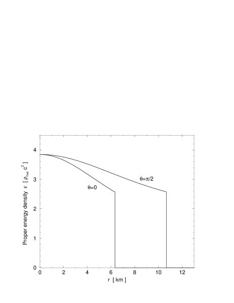
Figure 3: Profiles of the proper energy density $\epsilon$ in the equatorial plane ($\theta=\pi/2$) and along the rotation axis ($\theta=0$) for the rotating strange star model shown in Fig. 2.

3.3 Description of a typical model

A rapidly rotating strange star model obtained from the code is shown in Figs. 2 and 3. Assuming $B=60{\rm\ MeV\,fm}^{-3}$, this model has a baryon mass $M_{\rm B}=2.00\,{\rm M}_{\odot}$, a gravitational mass $M=1.60\,{\rm M}_{\odot}$, and a rotation period $P=0.87{\ \rm ms}$. The central baryon density is $n_{\rm c}=0.42{\rm\ fm}^{-3}$, the central values of the metric potentials $N$, $A$, $B$ and $N^{\varphi}$ [cf. Eq. (6)] are respectively 0.65, 1.47, 1.47 and $0.46\,\Omega$. The boundary between the computational domains D1 and D2 introduced in Sect. 3.2 coincides with the stellar surface (thick solid line in Fig. 2). The boundary between the computational domains D2 and D3 is out of the scope of the Figure. The energy density profile corresponding to this model is shown in Fig. 3. Note the strong discontinuity at the stellar surface: the jump in density is $\sim 2/3$ of the central density.

Figure 4: Same as Fig. 2 but for a strange star rotating at the Keplerian limit. The star’s baryon mass is $M_{\rm B}=2.34\,{\rm M}_{\odot}$, gravitational mass $M=1.89\,{\rm M}_{\odot}$, and rotation period $P=0.82{\ \rm ms}$. Thin dashed and solid lines are isocontours of the log-enthalpy $H$. Thin dashed lines correspond to negative values, and thin solid lines to positive values of $H$, respectively. The thick dot-dashed line denotes the boundary between the computational domains D1 and D2.

3.4 Treatment of configurations at the Keplerian limit

The maximum rotation rate that a star can sustain is reached when the velocity at the equator equals the velocity of an orbiting particle (a higher velocity would result in a centrifugal break-up of the star). This limit is called the Keplerian limit. It is reached when the derivative $\partial H/\partial r$ vanishes at the stellar equator. The surface of the star is then no longer smooth but exhibits a cusp along the equator (see Fig. 4). Such a non-differentiable surface cannot be decribed by the mapping (21)-(23) because the functions $F_{1}(\theta)$ and $F_{2}(\theta)$ are assumed to be expandable in $\cos(k\theta)$ series (cf. Bonazzola et al. (1998b)), which implies that they are smooth functions of $\theta$. The solution to this problem consists in freezing the adaptation of the mapping to the stellar surface when the ratio $(\partial H/\partial r)_{\rm eq}\;/\;(\partial H/\partial r)_{\rm pole}$ passes below a certain threshold during the iteration process. For instance, this threshold was chosen to be $0.28$ in the computation shown in Fig. 4. Consequently, in the final result, the density discontinuity at the stellar surface no longer coincides with the boundary between the computational domains D1 and D2, except at the equator. In this case, a Gibbs phenomenon is present. The accuracy of the calculation is then lower than when the mapping is adapted to the surface of the star. However, since the stellar interior covers most of domain D1 (cf. Fig. 4), the Gibbs phenomenon is rather limited. It is notably less severe than if D1 would have been a sphere of radius $r_{\rm eq}$, as in our previous numerical method (Bonazzola et al. 1993).

3.5 Tests of the numerical code

Various tests have been passed by the code. First of all, we recover previous results, e.g. those presented in Nozawa et al. (1998), when using an EOS for neutron star matter instead of the strange quark matter EOS presented in Sect. 2.

Regarding the treatment of the density discontinuity at the stellar surface, the code has been tested on the computation of MacLaurin ellipsoids (homogeneous rotating bodies in the Newtonian regime), and gives excellent results, as recalled in Sect. 3.2: the relative accuracy reaches $10^{-12}$ !

Another type of test is the evaluation of the virial identities GRV2 (Bonazzola 1973, Bonazzola & Gourgoulhon 1994) and GRV3 (Gourgoulhon & Bonazzola 1994), this latter being a relativistic generalization of the classical virial theorem. GRV2 and GRV3 are integral identities which must be satisfied by any solution of the Einstein equations (7)-(10) and which are not imposed during the numerical procedure (cf. Nozawa et al. 1998 for details on the computation of GRV2 and GRV3). When presenting numerical results, we will systematically give the accuracy by which the numerical solution satisfies these virial identities.

As discussed in Sect. 3.4, the computation of configurations rotating at the Keplerian limit is not free of Gibbs phenomenon. In order to gauge the resulting numerical error, we performed various computations of the same Keplerian configuration, by varying the numbers of coefficients in the spectral method and by varying the threshold on $(\partial H/\partial r)_{\rm eq}\;/\;(\partial H/\partial r)_{\rm pole}$ for freezing the mapping. We systematically used three sets of numbers of coefficients (= number of collocation points): $(N_{r},N_{\theta})$ = $(33,17)$, $(37,19)$ and $(41,21)$ in each of the three domains. The threshold on $(\partial H/\partial r)_{\rm eq}\;/\;(\partial H/\partial r)_{\rm pole}$ was varied from $0.28$ down to $0.20$. The variation of all these parameters lead to a relative change of the numerical solution of the order of or below $1\%$. This gives an estimation of the error of our method in computing strange stars at the Keplerian limit. Note the GRV2 and GRV3 errors for Keplerian configurations revealed to be better than this. For instance, for the configuration shown in Fig. 4, the GRV2 (resp. GRV3) error is $3\,10^{-5}$ (resp. $1.3\,10^{-3}$).

Figure 5: Rotating strange star configurations in the mass - central density plane. The static limit and Keplerian limit are denoted by thick solid lines. Thin solid lines denotes sequences of constant baryon number; they are labelled by the baryon mass (in ${\rm M}_{\odot}$ units). The dashed line marks the limit of stability with respect to axisymmetric pertubations; configuration to the right of the dashed line are (secularly) unstable. Its intersection with the Keplerian limit curve is marked by an open square. It is the location of the fastest rotating stable star. Maximum mass configurations are denoted by circles

4 Numerical results

4.1 General properties

For rigid rotation, the equilibrium configurations span a two-dimensional domain. This domain is shown in Fig. 5 in the central density - gravitational mass plane. Selected configurations are listed in Table 1. The symbols have the following meaning: $M$ is the gravitational mass; $M_{\rm B}$ is the baryon mass; $\Omega$ is the angular velocity, $P$ the corresponding rotation period; $n_{\rm c}$ is the central baryon density; $\rho_{\rm c}$ is the central proper energy density divided by $c^{2}$; $H_{\rm c}$ is the central log-enthalpy [Eq. (17)]; $R_{\rm eq}$ is the circumferential radius, i.e. the length of the equator [as given by the metric (6)] divided by $2\pi$; $r_{\rm eq}$ is the equator $r$ coordinate; $r_{\rm pole}/r_{\rm eq}$ is the coordinate oblateness of the star; $I$ is the moment of inertia (defined as $J/\Omega$); $J$ is the star angular momentum; $Q$ is the quadrupole moment defined as in Salgado et al. (1994a) or Laarakkers & Poisson (1999); $T/W$ is the “kinetic to gravitational energy” ratio (see Sect. 6); $U_{\rm eq}$ is the rotation velocity at the equator as measured by a locally non-rotating observer (those observer whose 4-velocity is the normal to the $t={\rm const}$ hypersurfaces); $z_{\rm eq}^{\rm f}$ is the redshift for an emission at the equator and in the direction of rotation, $z_{\rm eq}^{\rm b}$ the redshift for an emission at the equator and in the direction opposite to rotation, $z_{\rm pole}$ the redshift at the stellar pole; $N_{\rm c}$, $N^{\varphi}_{\rm c}$, $A_{\rm c}$ and $B_{\rm c}$ are the metric potentials [Eq. (6)] at the stellar center. Finally GRV2 and GRV3 are the two virial error indicators discussed in Sect. 3.5.

Table 1: Selected strange star models ($B=60{\rm\ MeV\,fm}^{-3}$); symbols are defined in Sect. 4.1.

Model	$M=1.4\,{\rm M}_{\odot}$	$M_{\rm max}^{\rm stat}$	$M=1.4\,{\rm M}_{\odot}$	$M_{\rm max}^{\rm rot}$	$\Omega_{\rm max}$
	$\Omega=0$		$P=1.56{\rm\ ms}$
$M$ [${\rm M}_{\odot}$]	1.400	1.964	1.400	2.831	2.822
$M_{\rm B}$ [${\rm M}_{\odot}$]	1.778	2.625	1.767	3.751	3.756
$\Omega$ [${\rm rad\,s}^{-1}$]	0	0	4028.	9547.	9916.
$P$ [ms]	-	-	1.560	0.6581	0.6337
$n_{\rm c}$ [${\rm fm}^{-3}$]	0.4842	1.110	0.4615	0.7486	0.8698
$\rho_{\rm c}$ [$10^{18}{\rm\ kg\,m}^{-3}$]	0.7524	2.059	0.7125	1.261	1.517
$H_{\rm c}$	0.1747	0.4514	0.1588	0.320	0.370
$R_{\rm eq}$ [km]	10.77	10.71	11.19	16.54	16.02
$r_{\rm eq}$ [km]	8.573	7.532	8.946	11.37	10.86
$r_{\rm pole}/r_{\rm eq}$	1.	1.	0.8935	0.4618	0.4762
$I$ [$10^{38}{\rm\ kg\,m}^{2}$]	1.492	2.155	1.603	6.534	6.101
$J$ $[G{\rm M}_{\odot}^{2}/c]$	0	0	0.7332	7.084	6.871
$cJ/(GM^{2})$	0	0	0.3741	0.8837	0.8625
$Q/(MR_{\rm eq}^{2})$	0	0	0.0250	0.0749	0.0713
$c^{4}Q/(G^{2}M^{3})$	0	0	0.7305	1.172	1.054
$T/W$	0	0	0.0348	0.2100	0.2007
$U_{\rm eq}$ [c]	0	0	0.1565	0.5731	0.5812
$z_{\rm eq}^{\rm f}$	0.2742	0.4768	0.0463	$-0.3608$	$-0.3634$
$z_{\rm eq}^{\rm b}$	0.2742	0.4768	0.5351	2.584	2.722
$z_{\rm pole}$	0.2742	0.4768	0.2825	0.8070	0.847
$N_{\rm c}$	0.6590	0.4312	0.6653	0.4019	0.374
$N^{\varphi}_{\rm c}/\Omega$	0	0	0.4203	0.7320	0.7540
$A_{\rm c}=B_{\rm c}$	1.439	1.914	1.432	2.135	2.234
GRV2	$1.\;10^{-12}$	$9.\;10^{-12}$	$1.\;10^{-4}$	$2.\;10^{-4}$	$9.\;10^{-4}$
GRV3	$2.\;10^{-12}$	$1.\;10^{-11}$	$2.\;10^{-4}$	$1.\;10^{-4}$	$2.\;10^{-3}$

Figure 6: Angular momentum as a function of the rotation frequency $f=\Omega/(2\pi)$ along sequences of constant baryon number. Each sequence is labelled by its baryon mass in ${\rm M}_{\odot}$ units. The heavy black circles denotes Keplerian configurations.

4.2 Evolutionary sequences

A strange star which slowly loses energy and angular momentum via electromagnetic or gravitational radiation keeps its total baryon number constant. Therefore, we can compute evolutionary sequences of strange stars as sequences at fixed baryon mass $M_{\rm B}$. Similarly to neutron stars, two categories of strange stars can be distinguished: normal stars, which have a baryon mass lower than the maximum baryon mass of static configurations $M_{\rm B,max}^{\rm stat}=2.625\,B_{60}^{-1/2}\;{\rm M}_{\odot}$ (cf. Table 1), and supramassive stars, which have a baryon mass greater than $M_{\rm B,max}^{\rm stat}$. Any normal star belongs to an evolutionary sequence which terminates at a static configuration. On the contrary, supramassive stars exist only by virtue of rotation. The two families clearly appear in Fig. 6, which is a plot of the angular momentum as a function of the rotation frequency for evolutionary sequences. The supramassive sequences are not connected with the static limit $\Omega=0$. At both ends, they terminate by Keplerian configuration. The limiting case $M_{\rm B}=M_{\rm B,max}^{\rm stat}$ is denoted by the thick line in Fig. 6.

A characteristic feature of some supramassive sequences also appears in Fig. 6: they can be spun-up by angular momentum loss: $d\Omega/dJ<0$. This effect is well known for Newtonian stars with soft EOS (adiabatic index close to $4/3$) (Shapiro et al. 1990), as well as for (relativistic) neutron stars (Cook et al. 1994, Salgado et al 1994a). As can be seen from Fig. 6, this effect is very prononced for strange stars.

Beside the fact that they can represent evolution path of rotating strange stars, another motivation for computing constant baryon number configurations is that this permits a stability analysis, as discussed in Sect. 5.1 below.

4.3 Comparison with previous works

First of all, in the non-rotating case, we recover the results presented in Haensel et al. (1986) for massless strange quarks [compare the $M_{\rm max}^{\rm stat}$ model in Table 1 with Eq. (28) of Haensel et al. (1986)].

The first rapidly rotating model of a strange star has been computed by Friedman (unpublished, quoted in Glendenning (1989a,b)). The obtained maximum angular velocity is $6\%$ lower than ours (last column in Table 1). The corresponding gravitational mass is $7\%$ lower than ours, and the central energy density is $7\%$ greater than ours.

The only other rapidly rotating model of strange star published in the literature is that of Lattimer et al. (1990). The maximum angular velocity obtained by these authors is $2\%$ lower than ours (last column in Table 1) . The corresponding mass is $12\%$ lower than ours, the circumferential radius $R_{\rm eq}$ $14\%$ lower, the ratio $T/W$ $10\%$ lower, and the polar redshift (linked to the injection energy $\beta$ given by Lattimer et al. (1990) by $z_{\rm pole}=\beta^{-1/2}-1$) $15\%$ lower. The largest discrepancy arises for the baryon mass $M_{\rm B}$: the value reported by Lattimer et al. (1990) is $21\%$ lower than ours. However we suspect some error in the presentation of the results by Lattimer et al. (1990), because (i) their ratio $M_{\rm B}/M$ is only $1.18$, whereas it is as large as $1.34$ for the non-rotating maximum mass model (for comparison, our value of $M_{\rm B}/M$ for the $\Omega_{\rm max}$ model is $1.35$), (ii) in the neutron star case, large discrepancies with baryon masses presented in Lattimer et al. (1990) have been noticed previously by Salgado et al. (1994a) [see Sect. 5.1.2 of Salgado et al. (1994a)]. Note that the numerical code employed by Salgado et al. (1994a) has been successfully compared with codes from two other groups in Nozawa et al. (1998) and did not show any trouble with the baryon mass. Unfortunately, the baryon mass of Friedman’s model is not reported in Glendenning (1989a,b).

Apart from the baryon mass problem discussed above, the discrepancy with Friedman and Lattimer et al. (1990) results remains rather large. It may be explained as follows. Both Friedman’s code [presented in Sect. II.a of Friedman et al. (1986)] and Lattimer et al. (1990) code employ the Butterworth & Ipser (1976) finite difference technique for numerically solving the partial differential equations resulting from Einstein’s equations. Butterworth & Ipser (1976) considered explicitly the case of a strong discontinuity in the density field at the stellar surface [their Sect. III.c)ii)]. However they treat it only along the radial direction (by using a modified Lagrangian-polynomial fit in $r$) and keep a Legendre expansion for the angular variable $\mu:=\cos\theta$. This is correct as long as the stellar surface is exactly spherical, i.e. the star is static. But when the surface deviates from spherical symmetry (as is the case for rapidly rotating stars, cf. Figs. 2 and 4), there is also a discontinuity in the $\theta$ direction. This discontinuity, when described by means of Legendre polynomials, which are smooth functions, inevitably generates spurious oscillations — the so-called Gibbs phenomenon. We believe that it is this Gibbs phenomenon which explains the discrepancy between Friedman and Lattimer et al. (1990) results and ours.

5 Maximally rotating configuration and scaling with $B$

5.1 Maximally rotating stable configuration

A natural bound on $\Omega$ results from the mass shedding condition, corresponding to the Keplerian angular velocity, $\Omega_{\rm K}$ discussed in Sect. 3.4: stationary configurations of uniformly rotating strange stars with $\Omega>\Omega_{\rm K}$ do not exist. We will also require, that the stationary, uniformly rotating configuration be stable with respect to axisymmetric perturbations (see e.g. Sect. 2.5.1 of Friedman 1998). We assume that the strange star is sufficiently hot, so that it is not subject to the r-mode instabilities (Madsen 1998). The maximum value of $\Omega$ for stationary, uniformly rotating models of strange stars which satisfy these two conditions, will be denoted by $\Omega_{\rm max}$, and the corresponding configuration will be called a maximally rotating one.

The stability with respect to axisymmetric perturbations can be investigated by means of the turning point theorem established by Friedman et al. (1988). We use the following variant of it [also used by Baumgarte et al. (1998)]: along an evolutionary sequence (i.e. a sequence at constant baryon number, Sect. 4.2), the change in stability is reached when the gravitational mass reaches a minimum. Using this criterion, we have determined the boundary separating stable and unstable configurations by linking the points of mimimum $M$ along the constant baryon mass sequences in Fig. 5: the configurations located to the left (resp. to the right) of the dashed line in Fig. 5 are stable (resp. unstable) with respect to axisymmetric perturbations. Moreover, the intersection of this line with the $\Omega=\Omega_{\rm K}$ line in Fig. 5 marks the maximum angular velocity allowable for stable rotating strange stars, i.e. the $\Omega_{\rm max}$ configuration. It is denoted by a square and is listed in the last column of Table 1.

As noted by Cook et al. (1994) and Stergioulas & Friedman (1995), the $\Omega_{\rm max}$ configuration and the configuration with maximum gravitational mass, $M_{\rm max}^{\rm rot}$, do not coincide, although they are close to each other for typical neutron star models. We also found this for rotating strange stars, and the effect is more pronounced than in the case of neutron stars: it can be seen easily in Fig. 5. The parameters of the $M_{\rm max}^{\rm rot}$ and $\Omega_{\rm max}$ configurations are listed in the last two columns in Table 1. $\Omega_{\rm max}$ is $4\%$ higher than $\Omega(M_{\rm max}^{\rm rot})$. Note that the $M_{\rm max}^{\rm rot}$ configuration is on the stable side, so that the situation is similar to that presented in Fig. 9 of Stergioulas & Friedman (1995), or Fig. 8 of Koranda et al. (1997).

5.2 Formulæ for $\Omega_{\rm max}$

The scaling properties of the equation of the stationary motion imply that $\Omega_{\rm max}\propto B^{1/2}$. The calculation of $\Omega_{\rm max}$ involves locating the threshold for the instability with respect to the axisymmetric perturbations, and requires therefore a higly precise numerical code for the 2-D calculations of stationary configurations. Therefore, the precision with which the scaling formula for $\Omega_{\rm max}$ is fulfilled reflects the overall precision of our numerical calculations. Our numerical results for $\Omega_{\rm max}$ can summarized in exact formulae

$$\Omega_{\rm max}=9.92\;10^{3}\leavevmode\nobreak\ \sqrt{B_{60}}{\rm\ rad\,s^{-1}}\leavevmode\nobreak\ ,\leavevmode\nobreak\ \leavevmode\nobreak\ P_{\rm min}={0.634\over\sqrt{B_{60}}}\leavevmode\nobreak\ {\rm ms}\leavevmode\nobreak\ .$$ (24)

We checked that the scaling $\Omega_{\rm max}\propto\sqrt{B}$ holds with a very high precision.

Within our simple model of EOS of strange matter, the constraints on the bag constant $B$, Sect. 2, imply

$$0.513\leavevmode\nobreak\ {\rm ms}<P_{\rm min}<0.640\leavevmode\nobreak\ {\rm ms}\leavevmode\nobreak\ .$$ (25)

In the case of dense baryon matter, exact results for the maximum rotation frequency of uniformly rotating neutron star models, for a very broad set of realistic causal EOS, show an interesting correlation with values of the mass and radius of the static configuration with maximum allowable mass, $M_{\rm max}^{{\rm stat}}$, $R_{M_{\rm max}}^{{\rm stat}}$ (Haensel & Zdunik 1989, Shapiro et al. 1989, Friedman et al. 1989, Friedman 1989, Haensel et al. 1995). The most recent form of such an “empirical formula” for $\Omega_{\rm max}$, derived in (Haensel et al. 1995), reads

$$\Omega_{\rm max} \simeq C_{\rm NS}\left({M_{\rm max}^{\rm stat}\over{\rm M}_{\odot}}\right)^{1\over 2}\left({R_{M_{\rm max}}^{\rm stat}\over 10\leavevmode\nobreak\ {\rm km}}\right)^{-{3\over 2}}\leavevmode\nobreak\ ,$$

$$C_{\rm NS} = 7730{\rm\ rad\,s^{-1}}\leavevmode\nobreak\ ,$$ (26)

where the prefactor $C_{\rm NS}$, which does not depend on the EOS of dense baryon matter, has been obtained via fitting “empirical formula” to exact numerical results for realistic, causal EOS of baryon matter. The “empirical formula” reproduces exact results with a surprisingly high precision, the relative deviations from Eq. (26) not exceeding 5%. In the case of strange stars, built of strange matter of massless quarks, the formula of the type (26) is exact, albeit with a different numerical prefactor. Using our numerical results, we get $C_{\rm SS}=7.84\leavevmode\nobreak\ 10^{3}\leavevmode\nobreak\ {{\rm rad}\over{\rm s}}$, so that $C_{\rm SS}\simeq C_{\rm NS}$ within better than 2%. Therefore, “empirical formula”, derived originally for (ordinary) neutron stars, holds also, with very good precision, for strange stars. Our conclusion agrees with unpublished result of Friedman (quoted in Glendenning 1989a), and with Lattimer et al. (1990).

5.3 Formulæ for maximum mass configurations

Rotation increases maximum allowable mass of strange stars, and the equatorial radius of the maximum mass configuration. Our results for the maximum mass of rotating configurations, $M_{\rm max}^{\rm rot}$, and its equatorial radius, $R_{{\rm eq},M_{\rm max}^{\rm rot}}$, can be summarized in two exact formulae,

$$M_{\rm max}^{\rm rot} = {2.831\over\sqrt{B_{60}}}\leavevmode\nobreak\ {\rm M}_{\odot}\leavevmode\nobreak\ ,$$

$$R_{{\rm eq},M_{\rm max}}^{\rm rot} = {16.54\over\sqrt{B_{60}}}\leavevmode\nobreak\ {\rm km}\,$$ (27)

The ratio of the maximum mass of rotating configurations to that of static ones, and the ratio of the corresponding equatorial radii, are thus independent of $B$,

$${M^{\rm rot}_{\rm max}\over M^{\rm stat}_{\rm max}}=1.44\leavevmode\nobreak\ ,\leavevmode\nobreak\ \leavevmode\nobreak\ {R_{{\rm eq},M_{\rm max}}^{\rm rot}\over R_{M_{\rm max}}^{\rm stat}}=1.54\leavevmode\nobreak\ .$$ (28)

It has been pointed out by Lasota et al. (1996), that for realistic causal baryonic EOS the ratios $M^{\rm rot}_{\rm max}/M^{\rm stat}_{\rm max}$ and $R_{{\rm eq},M_{\rm max}}^{\rm rot}/R_{M_{\rm max}}^{\rm stat}$ are very weakly dependent on the EOS, and can be very well approximated (within a few percent) by constants $C_{M}=1.18$ and $C_{R}=1.34$, respectively.

In the case of strange stars the values of $C_{M}$ and $C_{R}$ are significantly higher; rotation increases the value of $M_{\rm max}$ by 44% compared to 18% for neutron stars, while the corresponding increase in the equatorial radius is 54% compared to 34% for neutron stars.

We conclude that“empirical formula” for $\Omega_{\rm max}$ has more universal character than the “empirical formulae” for $M_{\rm max}^{\rm rot}$, $R_{{\rm eq},M_{\rm max}}^{\rm rot}$, proposed in Lasota et al. (1996); the former applies both for neutron and strange stars, while the latter describe neutron stars only.

6 About triaxial instabilities of rapidly rotating strange stars

6.1 Known results on the threshold in $T/W$ for triaxial instabilities

Rapidly rotating neutron stars can be subject to a spontaneous breaking of their symmetry about the rotation axis, resulting from some triaxial instability, when their rotation rate exceeds a certain threshold (see e.g. Bonazzola & Gourgoulhon (1997), Friedman (1998) or Stergioulas (1998) for a review). In order for the symmetry breaking to take place, a (secular) dissipative mechanism has to be working. Basically two such mechanisms can be contemplated: (i) viscosity and (ii) coupling with gravitational radiation (Chandrasekhar-Friedman-Schutz (CFS) instability). For compact stars that are accelerated by accretion in X-ray binary systems, these triaxial instabilities may be an important source of gravitational waves, in the frequency band of the LIGO/VIRGO interferometric detectors currently under construction. Another situation where these triaxial instabilities might develop is in compact stars newly formed after a stellar core gravitational collapse.

In the present paper, we have restricted ourselves to stationary and axisymmetric rotating strange star models. Therefore, we could not compute the triaxial instability threshold of rotating strange stars. However, an indicator of the stability of a rotating self-gravitating body is its kinetic to gravitational potential energy ratio $T/W$, which can be computed for any equilibrium configuration. For instance, it is well known that a homogeneous Newtonian rotating body (MacLaurin spheroid) becomes secularly unstable with respect to triaxial $\ell=m=2$ perturbations (bar mode) if $T/W>0.1375$ (Jacobi/Dedekind bifurcation point in the MacLaurin sequence). For compressible bodies (still in the Newtonian regime), this threshold can be lowered to $0.1275$ (Bonazzola et al. 1996). The threshold of the CFS instability decreases with the mode number $m$ for polar modes: for a Newtonian polytrope of abiabatic index $\gamma=2$, one has $T/W>0.079$ for a $m=3$ polar mode, $T/W>0.058$ for $m=4$ and $T/W>0.046$ for $m=5$ (Stergioulas & Friedman 1998). Higher order modes are likely to be damped out by viscosity. For axial r-modes, the CFS instability is generic, i.e. it occurs at any rotation rate (Andersson 1998). Madsen (1998) has however argued that the r-mode instability is suppressed by the quark matter bulk viscosity in new born strange stars.

In the relativistic case, a ratio $T/W$ can be defined according to Friedman et al. (1986) prescription. This quantity reduces to the usual kinetic to gravitational energy ratio at the Newtonian limit, whereas its physical interpretation in the relativistic case is not so clear (in particular the value of $T/W$ is coordinate dependent). However it can be used to measure the importance of rotational effects.

For the viscosity-driven instability, general relativistic terms increase the threshold on $T/W$: it becomes as high as $T/W>0.26$ for a compactification parameter $M/R=0.2$, according to the post-Newtonian analysis of Shapiro & Zane (1998). This stabilizing effect of general relativity onto the viscosity-driven bar instability has also been found by Bonazzola et al. (1998a).

On the contrary, general relativity decreases the threshold of the CFS instability, down to $T/W>0.065$ for $m=2$ polar mode (this mode being always stable in the Newtonian regime for $\gamma=2$), $T/W>0.046$ for $m=3$, $T/W>0.035$ for $m=4$, and $T/W>0.029$ for $m=5$, for a $\gamma=2$ polytrope [Stergioulas & Friedman 1998, see also Yoshida & Eriguchi (1997)].

Figure 7: Kinetic to gravitational energy ratio $T/W$ as a function of the rotation frequency $f=\Omega/(2\pi)$ along sequences of constant baryon number. Each sequence is labelled by its baryon mass in ${\rm M}_{\odot}$ units. The heavy black circles denotes Keplerian configurations.

6.2 $T/W$ ratio of rotating strange stars

Having the above results in mind, we have computed the $T/W$ ratio according to the prescription of Friedman et al. (1986), for each of our rotating stange star models. In particular, Fig. 7 shows the value of $T/W$ as a function of the rotation frequency along evolutionary sequences. It appears clearly that the values of $T/W$ for strange stars are much greater than for neutron stars (compare e.g. with Fig. 4 of Cook et al. (1994)). In particular, for the $\Omega_{\rm max}$ configuration,

$$\left({T\over W}\right)_{\Omega_{\rm max}}=0.201\leavevmode\nobreak\ ,$$ (29)

(it does not depend on $B$) whereas it ranges from $0.105$ to $0.139$ for the set of neutron star EOS examined in Nozawa et al. (1998). The fact that $T/W$ for maximally rotating strange stars is significantly larger than that for neutron stars, has been noted by Lattimer et al. (1990) and Colpi & Miller (1992).

Moreover, contrary to neutron stars, the value of $T/W$ remains very high, of the order of $0.2$, for rapidly rotating strange stars of moderate mass: the value $T/W=0.2$ is reached at a rotation period $P=0.86{\rm\ ms}$ (resp. $P=0.85{\ \rm ms}$) for a baryon mass of $M_{\rm B}=1.60\,{\rm M}_{\odot}$ (resp. $M_{\rm B}=1.80\,{\rm M}_{\odot}$), which corresponds to a gravitational mass $M=1.31\,{\rm M}_{\odot}$ (resp. $M=1.47\,{\rm M}_{\odot}$) (notice that in the static case $M_{\rm B}=1.6,\leavevmode\nobreak\ 1.8\leavevmode\nobreak\ {\rm M}_{\odot}$ for normal sequences in Fig. 7 correspond to gravitational masses $M=1.27,\leavevmode\nobreak\ 1.42\leavevmode\nobreak\ {\rm M}_{\odot}$, respectively).

All this seems to indicate that triaxial instabilities could develop more easily in rotating strange stars. However, it has to be stressed that no actual stability analysis has been performed yet for strange stars which, in contrast to ordinary neutron stars, are bound not only by gravity, but also by confinement forces. These confinement forces are represented represented by the bag pressure, $-B$, acting on the strange star surface. The density profiles, Fig. 3, and adiabatic index $\gamma$, Fig. 1, are qualitatively different from those characteristic of rotating neutron star models, for which triaxial instabilities have been studied.

7 Discussion and conclusions

The numerical method used in the present paper is particularly suitable for exact calculations of models of rapidly rotating strange stars. In contrast to numerical approaches used in previous calculations, the multi-domain method enabled us to treat exactly the huge density discontinuity at the surface of strange stars. We used three-domain grid in both $r$ and $\theta$ variables, adapted (adjusted) via a self-consistent procedure to the stationary shape of rotating strange star surface. The precision of our calculations was checked using several tests. We found significant differences between our results, and those obtained by other authors in previous exact calculations of the models of maximally rotating strange star models.

As noted in the early papers on the properties of strange stars, models of static massive ($M\ga{\rm M}_{\odot}$) strange stars are characterized by global stellar parameters (mass, radius, moment of inertia, surface redshift) which are rather similar to those of ordinary neutron stars (Haensel et al. 1986, Alcock et al. 1986). In contrast to the static case, rapidly rotating strange stars exhibit qualitative differences with respect to rapidly rotating neutron stars.

Strange stars rotating close to the break up (Keplerian) frequency have kinetic to gravitational energy ratio $T/W\simeq 0.2$, which is nearly twice larger than corresponding values for neutron stars. Moreover, this unusually high $T/W\sim 0.2$ is characteristic not exclusively for supermassive rotating models, but is typical also for normal rotating configurations with baryon mass lower than the maximum allowed mass for static models. In particular, $T/W\simeq 0.2$ is reached for the $1.4\leavevmode\nobreak\ {\rm M}_{\odot}$ models rotating at $P\simeq 0.85\leavevmode\nobreak\$ms. Large value of $T/W$ stems from a flat density profile combined with strong equatorial flattening of rapidly rotating strange stars. These particular features of rapidly rotating strange stars are consequences of a special character of EOS of strange quark matter in the strange star interior, reflected by a specific density dependence of the adiabatic index. Strange matter inside massive ($M>{\rm M}_{\odot}$) strange stars is very stiff in the outer (surface) layers and soft in the central core. Large value of $T/W$ may signal a relative softness (susceptibility) of rapidly rotating strange stars to triaxial instabilities.

For simple strange matter EOS, used in the present paper, several exact scaling relations hold for extremal (maximum frequency, maximum mass) configurations of rotating strange stars. Maximum rotation frequency as well as maximum mass of rotating configurations exhibit an exact scaling with respect to the value of the bag constant. Empirical formula for $\Omega_{\rm max}$ for neutron stars, which relates this quantity to the mass and radius of static configuration with maximum allowable mass, holds with a high precision also for strange stars.

Minimum period of rotating strange stars, stable with respect to axisymmetric perturbations, obtained for an acceptable range of the bag constant, is $\simeq 0.5\leavevmode\nobreak\$ms, and therefore similar to that characteristic of realistic models of neutron stars. However, the effect of rapid rotation on the maximum allowable mass is significantly larger for strange stars than for neutron stars. Uniform rotation can increase the massimum allowable mass of strange stars by more than $40\%$, to be compared with only 20% increase for realistic models of neutron stars.

It should be stressed, that our numerical results for rapidly rotating strange stars, summarized in Eqs.(24,25), and Eqs.(27,28,29), have been obtained for a schematic EOS, Eq.(3). This particular EOS has been selected for the sake of simplicity and, last but not the least, for numerical convenience. The most general - generic - feature of an EOS of strange matter is the existence of a self-bound state at zero pressure, with $E_{0}<930.4$ MeV. However, the actual EOS of strange matter - should it exist - is expected to be different from that given by Eq.(3). Therefore, results of the present paper neither represent the full range of possibilities for “theoretical” strange stars, nor they are expected to correspond to precise actual values of parameters of rapidly rotating strange stars - should they exist in Nature.

The equation of state of strange matter, used in the present paper, has been derived neglecting strange quark mass and representing all effects of QCD interactions by one parameter - the bag constant $B$. However, this simplest (minimal) model exhibits generic properties of the EOS of a self-bound quark matter. Generally, inclusion of perturbative corrections, expressed in terms of the QCD coupling constant $\alpha_{\rm c}$, and of the strange quark mass $m_{s}$, imply shifting down and simultaneous narrowing of the window of the values of $B$ compatible with strange matter hypothesis (Farhi & Jaffe 1984). Typical values of $m_{s}$ are $\sim 200\leavevmode\nobreak\ {\rm MeV}/c^{2}$; the effect of $\alpha_{\rm c}\la 0.3$ on the EOS is then much smaller than that of $m_{s}$. Scaling relations between extremal strange star configurations, corresponding to different values of $B$ (at fixed values of $\alpha_{\rm c}$, $m_{s}$) are than no longer exact. In the case of static strange star models, they are still very precise (after the prefactors in these relations have been recalculated to include the effect of $\alpha_{\rm c}$ and $m_{s}$) and therefore useful (Haensel et al. 1986); similar situation is expected to take place in the case of rotating strange star models. In the static case, the effect of non-zero $m_{s}$ and $\alpha_{\rm c}$ consisted in making the maximum mass configurations less massive but more compact, and we expect similar effect for the extremal configurations of rotating strange stars.

In this paper we restricted ourselves to the case of strange stars with superdense quark surface, built exclusively of strange quark matter (bare strange stars). In principle, one should consider also models of strange stars, covered by an envelope (crust) consisting of nuclei immersed in electron gas (Alcock et al. 1986). The nuclei, forming a crystal lattice of the crust, are separated from strange matter by a repulsive coulomb barrier. Both coulomb barrier, and characteristic spatial gap between nuclei and strange matter, result from an electric dipole layer on the quark surface, due to the nonuniform density distribution of electrons near the quark surface. The presence of electrons in strange matter, necessary for equilibrium of quark core core with crust, results from nonzero strange quark mass. The maximum mass of the crust on a $M>{\rm M_{\odot}}$ strange star was originally estimated as $\sim 10^{-5}\leavevmode\nobreak\ {\rm M_{\odot}}$ (Alcock et al. 1986). Further studies of the crust–strange matter coexistence conditions led to an even lower value of the maximum mass of the crust on a $M>{\rm M}_{\odot}$ strange star, of the order of $10^{-6}\leavevmode\nobreak\ {\rm M}_{\odot}$ (Huang & Lu 1997).

In the case of the static strange star models, the effect of the presence of the crust on the maximum allowable mass configuration is very small. Rapid rotation will increase the maximum mass of a strange star crust (Glendenning & Weber 1992), but still its effect on the maximally rotating and maximum mass configurations may be expected to be small: both $\Omega_{\rm max}$ and $M_{\rm max}^{\rm rot}$ will be slightly reduced, as compared with the case of bare strange stars. It should be stressed, that the only existing calculation of rapid rotation of strange stars with crust (Glendenning & Weber 1992) was performed within a version of slow rotation approximation. The multi-domain method with adaptable grid, used in the present paper, is also suitable for an exact treatment of rapid rotation of strange stars with crust, in which matter density exhibits a huge discontinuity at the quark matter–crust interface, with outward density drop by more than three orders of magnitude. This problem is now being investigated.

- (1) Alcock C., Farhi C.E., Olinto A., 1986, ApJ 310, 261
- (2) Alpar M.A., 1987, Phys. Rev. Lett. 58, 2512
- (3) Andersson N., 1998, ApJ 502, 708
- (4) Baumgarte T.W., Cook G.B., Scheel M.A., Shapiro S.L., Teukolsky S.A., 1998, Phys. Rev. D 57, 6181
- (5) Bodmer A.R., 1971, Phys. Rev. D 4, 1601
- (6) Bombaci I., 1997, Phys. Rev. C 55, 1587
- (7) Bonazzola S., 1973, ApJ 182, 335
- (8) Bonazzola S., Gourgoulhon E., 1994, Class. Quantum Grav. 11, 1775
- (9) Bonazzola S., Gourgoulhon E., 1997, in Relativistic gravitation and gravitational radiation, Marck J.-A. & Lasota J.-P. (eds.). Cambridge University Press, Cambridge
- (10) Bonazzola S., Frieben J., Gourgoulhon E., 1996, ApJ 460, 379
- (11) Bonazzola S., Frieben J., Gourgoulhon E., 1998a, A&A 331, 280
- (12) Bonazzola S., Gourgoulhon E., Marck J.A., 1998b, Phys. Rev. D 58, 104020
- (13) Bonazzola S., Gourgoulhon E., Marck J.A., 1999, J. Comput. Appl. Math., in press, preprint: gr-qc/9811089
- (14) Bonazzola S., Gourgoulhon E., Salgado M., Marck J.A., 1993, A&A 278, 421
- (15) Butterworth E.M., Ipser J.R., 1976, ApJ 204, 200
- (16) Caldwell R.R., Friedman J.L., 1991, Phys. Lett. 264B, 143
- (17) Cheng K.S., Dai Z.G., Wei D.M., Lu T., 1998, Science 280, 407
- (18) Colpi M., Miller J.C., 1992, ApJ 388, 513
- (19) Cook G.B., Shapiro S.L., Teukolsky S.A., 1994, ApJ 424, 823
- (20) Dai Z.G., Lu T., 1998, Phys. Rev. Lett. 81, 4301
- (21) Farhi E., Jaffe R.L., 1984, Phys. Rev. D 30, 2379
- (22) Friedman J.L., 1989, General Relativity and Gravitation, Asby N., Bartlett D.F., Wyss W. (eds). Cambridge University Press, p. 21
- (23) Friedman J.L., 1998, in Black holes and relativistic stars, Wald R.M. (ed.). University of Chicago Press, Chicago
- (24) Friedman J.L., Ipser J.R., Parker L., 1986, ApJ 304, 115; errata published in ApJ 351, 705 (1990)
- (25) Friedman J.L., Ipser J.R., Parker L., 1989, Phys. Rev. Lett. 62, 3015
- (26) Friedman J.L., Ipser J.R., Sorkin R.D., 1988, ApJ 325, 722
- (27) Frieman J.A., Olinto A.V., 1989, Nature 341, 633
- (28) Glendenning N.K., 1989a, J. Phys. G.: Nucl. Part. Phys., 15, L255
- (29) Glendenning N.K., 1989b, Phys. Rev. Lett. 63, 2629
- (30) Glendenning N.K., Weber F., 1992, ApJ 400, 647
- (31) Glendenning N.K., 1997, Compact Stars: Nuclear Physics, Particle Physics and General Relativity, Springer, New York
- (32) Gourgoulhon E., Bonazzola S., 1994, Class. Quantum Grav. 11, 443
- (33) Goussard J.-O., Haensel P., Zdunik J.L., 1997, A&A 321, 822
- (34) Goussard J.-O., Haensel P., Zdunik J.L., 1998, A&A 330, 1005
- (35) Haensel P., Salgado M., Bonazzola S., 1995, A&A 296, 745
- (36) Haensel P., Zdunik J.L., 1989, Nature 340, 241
- (37) Haensel P., Zdunik J.L., Schaeffer R., 1986, A&A, 160, 121
- (38) Hartle J.B., 1967, ApJ 150, 1005
- (39) Hartle N.B, 1973, Ap&SS 24, 385
- (40) Hartle J.B., Thorne K.S., 1968, ApJ 153, 807
- (41) Huang Y.F., Lu T., 1997, A&A, 325, 189
- (42) Koranda S., Stergioulas N., Friedman J.L., 1997, ApJ 488, 799
- (43) Laarakkers W.G., Poisson E., 1999, ApJ 512, 282
- (44) Lasota J.-P., Haensel P., Abramowicz A.M., 1996, ApJ 456, 300
- (45) Lattimer J.M., Prakash M., Masak D., Yahil A., 1990, ApJ 355, 241
- (46) Madsen J., Haensel P., eds., 1991, Strange Quark Matter in Physics and Astrophysics (Nucl. Phys. B [Proc. Suppl.] 24B)
- (47) Madsen J., 1998, Phys. Rev. Lett. 81, 3311
- (48) Madsen J., 1999, in Hadrons in Dense Matter and Hadrosynthesis, Lecture Notes in Physics, Cleymans J. (ed.). Springer-Verlag, in press. Preprint: astro-ph/9809032
- (49) Nozawa T., Stergioulas N., Gourgoulhon E., Eriguchi Y., 1998, A&AS 132, 431
- (50) Prakash M., Baron E., Prakash M, 1990, Phys. Lett. B 243, 175
- (51) Salgado M., Bonazzola S., Gourgoulhon E., Haensel P., 1994a, A&A 291, 155
- (52) Salgado M., Bonazzola S., Gourgoulhon E., Haensel P., 1994b, A&AS 108, 455
- (53) Shapiro S.L., Teukolsky S.A., Nakamura T., 1990, ApJ 357, L17
- (54) Shapiro S.L., Zane S., 1998, ApJS 117, 531
- (55) Stergioulas N., 1998, Living Reviews in Relativity 1, 1998-8 (http://www.livingreviews.org/)
- (56) Stergioulas N., Friedman J.L., 1995, ApJ 444, 306
- (57) Stergioulas N., Friedman J.L., 1998, ApJ 492, 301
- (58) Weber F., Glendenning N.K., 1991, Phys. Lett. B, 265, 1
- (59) Weber F., Glendenning N.K., 1992, ApJ 390, 541
- (60) Weber F., Schaab Ch., Weigel M.K., Glendenning N.K., 1995, in Proceedings of the International Symposium on Strangeness and Quark Matter, Vassiliadis G., Panagiotou A., Kumar S., Madsen J. (eds.), World Scientific, Singapore, p. 322
- (61) Witten E., 1984, Phys. Rev. D 30, 272
- (62) Yoshida S., Eriguchi Y., 1997, ApJ 490, 779
- (63) Zdunik J.L., Haensel P., 1990, Phys. Rev. D 42, 710