Hydrodynamical simulations of the Sunyaev–Zel’dovich effect

Abstract

With detections of the Sunyaev–Zel’dovich (SZ) effect induced by galaxy clusters becoming routine, it is crucial to establish accurate theoretical predictions. We use a hydrodynamical $N$-body code to generate simulated maps, of size one square degree, of the thermal SZ effect. This is done for three different cosmologies — the currently-favoured low-density model with a cosmological constant, a critical-density model and a low-density open model. We stack simulation boxes corresponding to different redshifts in order to include contributions to the Compton $y$-parameter out to the highest necessary redshifts. Our main results are:

1. The mean $y$-distortion is around $4\times 10^{-6}$ for low-density cosmologies, and $1\times 10^{-6}$ for critical density. These are below current limits, but not by a wide margin in the former case.

2. In low-density cosmologies, the mean $y$-distortion is contributed across a broad range of redshifts, with the bulk coming from $z\la 2$ and a tail out to $z\sim 5$. For critical-density models, most of the contribution comes from $z<1$.

3. The number of SZ sources above a given $y$ depends strongly on instrument resolution. For a one arcminute beam, there is around 0.1 sources per square degree with $y>10^{-5}$ in a critical-density Universe, and around 8 such sources per square degree in low-density models. Low-density models with and without a cosmological constant give very similar results.

4. We estimate that the Planck satellite will be able to see of order 25000 SZ sources if the Universe has a low density, or around 10000 if it has critical density.

1 Introduction

The Sunyaev–Zel’dovich (SZ) effect (Sunyaev & Zel’dovich 1972, 1980; for reviews see Rephaeli 1995 and Birkinshaw 1999) is the change in energy experienced by cosmic microwave background photons when they scatter from hot gas, especially that in galaxy clusters. It comes in two forms. The dominant contribution is the thermal SZ effect, the gain in energy acquired from the thermal motion of the gas which is commonly at a temperature of tens of millions of degrees in clusters. It is described by the Compton $y$-parameter, also known as the $y$-distortion. The kinetic SZ effect is the Doppler shift arising from the bulk motion of the gas.

Since the first claimed detection by Parijskij (1972), and the more recent pioneering work of Birkinshaw, Hughes & Arnaud (1991) and Birkinshaw & Hughes (1994), detections of the thermal SZ effect from clusters have become routine. A number of instruments have become capable of making two dimensional maps, including the Ryle telescope, centimetre receivers on BIMA and OVRO, Viper, SuZie, SEST, PRONAOS and Diabolo. A blank-field survey has been proposed (Carlstrom et al. 1999), and eventually the Planck satellite will produce an all-sky catalogue likely to contain thousands of SZ sources.

Because clusters of galaxies are in the tail of the Universe’s mass distribution function, their number density is highly sensitive to the growth rate of density perturbations, which is governed primarily by the density parameter $\Omega_{0}$, but also influenced to a lesser extent by the density, $\Omega_{\Lambda}\equiv\Lambda/3H^{2}$, contributed by a cosmological constant $\Lambda$. Korolev, Sunyaev & Yakubtsev (1986) were the first to point out the interest of the SZ cluster source counts as a cosmological probe. Since then, a plethora of authors using a variety of techniques have discussed how the cosmological cluster evolution could be revealed by the SZ effect (Cole & Kaiser 1988; Cavalieri, Menci & Setti 1991; Markevitch et al. 1991, 1992, 1994; Bartlett & Silk 1994; Barbosa et al. 1996; Eke, Cole & Frenk 1996; Aghanim et al. 1997) and how gas evolution could mask it (Bartlett & Silk 1994; Colafrancesco et al. 1994, 1997).

Where the above-mentioned authors used extrapolations based on the known cluster X-ray luminosity functions to estimate the source counts, the preferred tool was without doubt the Press–Schechter (1974) approximation. Although in excellent agreement when compared to previous numerical simulations, its ansatz usually assumes that clusters can be modelled by some spherical, and usually isothermal, matter distribution. The maturity of this field now demands a sophisticated approach to the theoretical modelling of the effect, using hydrodynamical $N$-body simulations. The pioneering study of this kind, using a crude ‘sticky particle’ method, was by Thomas & Carlberg (1989) who made maps with one arcminute resolution. Cen & Ostriker (1992) used an Eulerian hydrodynamic code in order to study the mean $y$-distortion, and this was followed by Scaramella, Cen & Ostriker (1993) who used these simulations to make maps, using the standard Cold Dark Matter model which is however now excluded by observations. Persi et al. (1995) used hydrodynamic simulations as part of a semi-analytic calculation of the anisotropy power spectrum from the SZ effect. Hydrodynamic simulations have also been used to examine the properties of individual clusters (Metzler 1998), in particular seeking the relationship between $y$ and the cluster mass $M$. In this paper, we make simulated maps of the SZ effect, using state-of-the-art SPH hydrodynamical simulation techniques. This is done for three currently-popular cosmologies, enabling a comparison between them. These maps are of particular importance to simulate the SZ sky that near-future experiments will observe.

2 The simulations

Viable cosmological models must be able to reproduce the number density of clusters seen at the present epoch, which is quite well constrained observationally. However, in a map of a given angular size one expects most SZ clusters to be at quite significant redshifts, where observations have yet to constrain the number of clusters; consequently predictions become quite model dependent and one needs to consider several different models. Primarily, the number of clusters depends on the density parameter $\Omega_{0}$, with less prominent dependence on the cosmological constant $\Lambda$; assuming gaussian initial perturbations these are the only significant quantities as they determine the growth rate of density perturbations and hence the epoch of cluster formation.

We therefore consider three models, all from the cold dark matter (CDM) family. In each case the power spectrum was that of CDM with shape parameter $\Gamma=0.21$, and the normalization $\sigma_{8}$ was chosen to ensure good agreement with the present cluster number density (see e.g. Viana & Liddle 1999). The baryon density $\Omega_{{\rm B}}$ was chosen to agree with nucleosynthesis for a reasonable choice of the Hubble parameter $h$; we used $\Omega_{{\rm B}}h^{2}=0.02$, with $h=0.71$ for the low-density cosmologies and $h=0.50$ for the critical-density model. As cooling is not included, the simulations scale and for them $h$ need not be specified. However, since the $y$-distortion parameter is an integral along the line of sight, $h$ is required. How the derived $y$ varies with $h$ depends on how one chooses to scale the baryon density. If $\Omega_{{\rm B}}$ were fixed (preserving the gravitational forces), then the electron density $n_{{\rm e}}$ scales as $h^{2}$ and the scaling is $y\propto h$. However if we regard the gravitational effects of baryons as negligible, we could instead keep $\Omega_{{\rm B}}$ at the nucleosynthesis value and then $n_{{\rm e}}$ is independent of $h$ and the scaling is $y\propto h^{-1}$.

The models we use are

• $\Lambda$CDM: a low-density model with a flat spatial geometry and $\Omega_{0}=0.35$ and $\Omega_{\Lambda}=0.65$.

• $\tau$CDM: a critical-density model with $\Omega_{0}=1$ and $\Omega_{\Lambda}=0$.

• OCDM: a low-density open model with $\Omega_{0}=0.35$ and $\Omega_{\Lambda}=0$.

Current observational prejudice is in favour of the low-density flat model, and where we display results only for a single cosmology that is the one chosen.

The simulations were carried out using the public domain Hydra code (Adaptive P³M-SPH: Couchman, Thomas & Pearce 1995). In each case the box-size was $150\,h^{-1}$ Mpc, and equal numbers of dark matter and gas particles were used. The number of particles $N$ was chosen so as to keep the mass of the dark matter particles, $m_{{\rm dark}}=4.45\times 10^{11}\,h^{-1}M_{\odot}$, the same in each simulation. The same realization of the power spectrum was used in each case, though $\tau$CDM, having more particles, better samples the small-scale power. The softening was set at 40$\,h^{-1}$kpc. The other simulation parameters are given in Table 1. The effective resolution for the baryonic component is 32 times the gas particle mass, about $10^{12}M_{\odot}$.

The closest antecedent to this work is the excellent paper of Scaramella et al. (1993). They carried out a large number of separate simulations, but because of the poorer resolution computationally accessible at that time, these had sizes ranging from just $4\,h^{-1}$ Mpc to $64\,h^{-1}$ Mpc. Because of this, their simulations were significantly lacking in large-scale power and there were too few rich clusters. Although we only carry out a single simulation for each cosmology, this is of much greater volume and with higher resolution. In total, the volume of the Universe we simulate is comparable to theirs, but our large boxes contain all the necessary large-scale power, and allow a number of statistically independent lines of sight to be traced through them. Also, they only simulated the Standard CDM cosmology, which has since been shown to be a poor fit to observations; our three models provide good fits to current large-scale structure observations, especially the nearby cluster number density.

Table 1: The cosmological and numerical parameters for the simulations.

Model	$\Omega_{0}$	$\Omega_{\Lambda,0}$	$\Omega_{{\rm B},0}$	$\sigma_{8}$	$N/2$	$m_{{\rm gas}}/h^{-1}M_{\odot}$
$\Lambda$CDM	0.35	0.65	0.038	0.92	$90^{3}$	$4.85\times 10^{10}$
$\tau$CDM	1	0	0.08	0.56	$128^{3}$	$3.55\times 10^{10}$
OCDM	0.35	0	0.038	0.80	$90^{3}$	$4.85\times 10^{10}$

3 The map-making technique

3.1 SZ basics

The thermal SZ effect in a given direction is computed as a line integral, which gives the Compton $y$-parameter

$$y=\int{{k_{{\rm B}}\sigma_{{\rm T}}}\over{m_{{\rm e}}c^{2}}}\,\,T_{{\rm e}}\,n_{{\rm e}}\,dl\,.$$ (1)

In this expression $T_{{\rm e}}$ and $n_{{\rm e}}$ are the temperature and density of the electrons, $\sigma_{{\rm T}}=6.65\times 10^{-25}\,{\rm cm}^{2}$ the Thomson cross-section, $c$ the speed of light and $m_{{\rm e}}$ the electron rest mass. Usually, observers prefer to quote either the “SZ flux” at frequency $\nu$ on a line of sight,

$$S_{\nu}=j(x)\,y\,,$$ (2)

where $x=h\nu/kT_{\gamma}$ is the dimensionless frequency and the function $j(x)$ is the well-known frequency dependence of the thermal SZ effect accounting for the decrement or increment in flux with respect to the mean CMB background flux [Sunyaev & Zel’dovich 1972, Birkinshaw 1999], or to quote the temperature fluctuation given by

$$\frac{\Delta T}{T}=y\,\left[\frac{x}{\tanh(x/2)}-4\right]\,.$$ (3)

In the long-wavelength limit $x\ll 1$ (the Rayleigh–Jeans portion of the spectrum), this reduces to $\Delta T/T\simeq-2y$.

The simulation output is a set of particles with positions, velocities and temperatures. Each particle occupies a volume with a radius proportional to its SPH smoothing length, $h_{\rm i}$. Inside this volume we choose a mass profile given by $m_{{\rm gas}}W({\bf r}-{\bf r}_{\rm i},h_{\rm i})$, where ${\bf r}_{\rm i}$ is the position of the particle’s centre, $m_{{\rm gas}}$ is the mass of the gas particle and $W$ is the normalized spherically–symmetric smoothing kernel adopted in the simulations

$$W(x,h_{\rm i})={1\over{4\pi h_{\rm i}^{3}}}\left\{\matrix{4-6x^{2}+3x^{3}\;,\quad 0\leq x\leq 1\hfill\cr{(2-x)}^{3}\;,\quad\quad\quad\kern 1.0pt\,\,1<x\leq 2\hfill\cr 0\;,\quad\quad\quad\kern 1.0pt\quad\quad\;\;\;\;\,x>2\hfill\cr}\right.$$ (4)

where $x=\left|{{\bf r}-{\bf r}_{\rm i}}\right|/h_{\rm i}$. In order to evaluate $y$ in a single map pixel, we discretize the SZ integral into cubes of volume $V$ along the line of sight. If $A$ is the pixel area, then equation (1) can be rewritten as

$$y = {{k_{{\rm B}}\sigma_{{\rm T}}}\over{m_{{\rm e}}c^{2}}}\,\frac{1}{A}\,\int\,T_{{\rm e}}n_{{\rm e}}\,dV$$ (5)

$$= {k_{{\rm B}}\sigma_{{\rm T}}\over{m_{{\rm e}}c^{2}}}\,\frac{V}{A}\,{0.88\,m_{{\rm gas}}\over{m_{{\rm p}}}}\sum\limits_{\alpha}\sum\limits_{\rm i}T_{\rm i}W(\left|{{\bf r_{\alpha}}-{\bf r}_{\rm i}}\right|,h_{\rm i})\,,$$

where the $i$ sum runs over all particles which contribute to the pixel column, and the $\alpha$ sum is over the line of sight cubes. Here, $T_{\rm i}$ is the temperature of the gas particles, $m_{{\rm p}}$ is the proton mass, and the factor 0.88 gives the number of electrons per baryon, assuming a 24 per cent helium fraction and complete ionization in the regions of interest (guaranteed as regions have to be hot to contribute significantly to the SZ signal). The ratio of ionized electrons per baryon will vary modestly as metallicity builds up, but the effect is negligible in this context.

3.2 Map making

In order to make a realistic map, one must go to high enough redshift to ensure that all contributions are included. The brightest SZ sources tend to be quite nearby, but our aim is to make maps down to a low threshold, $y\ga 10^{-6}$, and with high angular resolution. The contribution from high redshifts dies off because structure formation is less advanced, but this is partly offset by two related effects. For a given mass, high-redshift objects are both hotter and more concentrated, as the Universe was smaller when they formed. For instance, the spherical collapse model predicts that for a given mass the temperature goes as $T\propto(1+z_{{\rm vir}})$, while the physical radius is smaller by a factor $1/(1+z_{{\rm vir}})$, where $z_{{\rm vir}}$ is the redshift of virialization. In combination, these effects mean that quite low mass objects can be seen at high redshift provided the angular resolution is high enough.

To go to the necessary redshift, we stack simulation boxes in a line extending to high redshift, as done by Thomas & Carlberg (1989) and Scaramella et al. (1993). Computational resources do not allow us to make separate simulations for each of the required boxes, but we are able to use outputs of a single simulation across a wide range of redshifts. This strategy is clearly not ideal, because the simulation boxes are not independent realizations, though we aim to minimize the relation between boxes by randomly translating (using the periodic boundary conditions of the simulation), reflecting and rotating the boxes before stacking. Further, the SZ sources we are seeking are primarily a short-scale phenomenon and the compromise is much less severe than were one aiming to compute, for example, a correlation function. Also, the map dimensions are determined so that the most distant considered box subtends close to the entire map area, which means that by the time one gets to the nearby boxes only a small fraction of their volume is being sampled so the nearest boxes are in effect independent — see Figure 1.

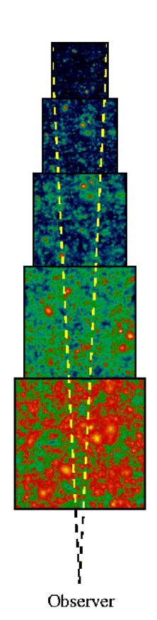
Figure 1: A schematic of the stacking of simulation boxes to make a map, in physical coordinates. Our actual stackings are of around 40 boxes. The observer is located at the centre of the redshift zero box, which we don’t include. Notice that only a small fraction of the volume of the nearby boxes contributes to the maps.

The redshifts of the simulation outputs were arranged so that the boxes fit together; our stackings include 48, 33 and 39 boxes for the flat, critical-density and open cosmologies respectively. We select a map size which is exactly one degree on a side, and include all boxes close enough to subtend an angular scale greater than this. We begin at redshift greater than 15; however as we will see the contribution from the boxes is negligible until redshifts around 5 for low-density models and even less with critical density. For each box, the angular diameter distance $d_{A}$ is computed, to indicate which fraction of the box will contribute to the map; for the most distant ones almost the entire volume contributes, while for the nearest almost none does. Within each box we use a small-angle approximation, computing an SZ map for that individual box by projecting onto a plane located at the centre of the box. These maps are made with $300\times 300$ pixels, corresponding to an angular resolution of 0.2 arcminutes. The final map is obtained by summing together the individual maps. The contribution from distant boxes is small because the material within them is not hot enough to give a significant effect, while that from nearby boxes is small because such a small volume within them is being probed that there is little chance of encountering a cluster.

Although we only possess one simulation for each of the three cosmologies, we are able to make several maps from each by choosing a different sequence of random translations, rotations and reflections for each box as it is stacked. We make 30 maps for each cosmology. While these maps are not truly independent, they give some flavour of the scatter were one to look to different regions of the sky. For example, in some realizations, by chance an SZ-bright nearby cluster appears while in most there are no prominent nearby clusters. Note that for the box at redshift one, which is around the mean redshift of contribution for the low-density flat cosmology, only 6 per cent of its volume contributes to the map, so separate map realizations are more independent than one might naively expect. Indeed, in the $\Lambda$CDM cosmology one has to go to $z=1.67$ for the accumulated volume contributing to the maps to reach the simulation volume.

In order to give results roughly corresponding to different instrument configurations, having made the maps we then smooth them with gaussians of various widths.

4 Results

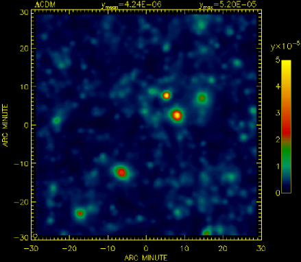
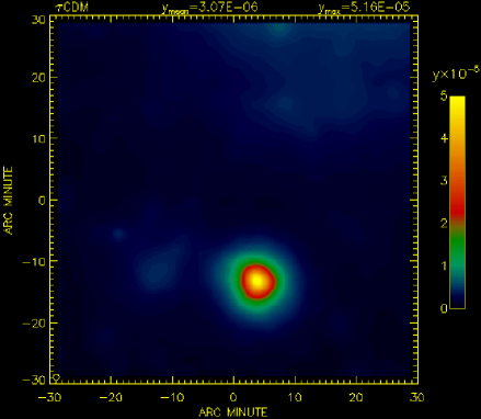
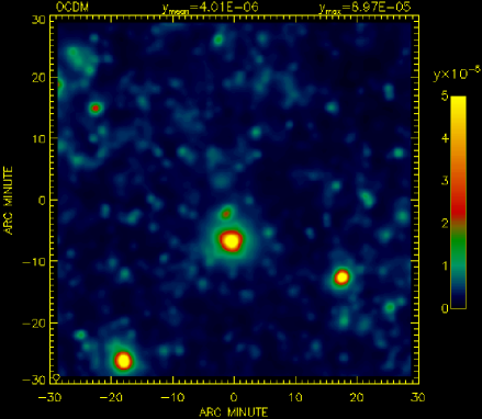
Figure 2: Simulated thermal SZ maps, showing the $y$-parameter in a patch of one square degree. In each case, the original map was convolved with a gaussian beam profile of FWHM = 1′. From top to bottom they are $\Lambda$CDM, $\tau$CDM and OCDM. The small circles in the bottom left of each image indicate the smoothing scale.

Typical example maps in each cosmology are shown in Figure 2, with the same colour scale in each. The original maps have been smoothed using a gaussian with a full-width half-maximum (FWHM) of 1′, comparable to the angular resolution of the best existing experiments. The visual appearance of the two low-density maps is rather similar, with several obvious bright spots, corresponding to clusters, as well as large numbers of fainter sources which collectively add up to give the mean distortions quoted below. Plotted with the same colour scale, the critical-density map clearly shows significantly less structure, which is due to the absence of high-redshift structures as compared to the low-density cases. Note that this particular critical-density map features a nearby large cluster; only about ten per cent of realizations for critical density show such a feature.

4.1 The mean distortion

The cumulative effect of hot gas, averaged over directions, gives rise to a mean $y$-distortion across the sky. We see from the maps that, especially in the low-density cases, there is a significant distortion along a large fraction of lines of sight. The best observational limit on the mean $y$-distortion comes from the COBE–FIRAS experiment, which sets a 95 per cent upper limit of $y_{{\rm mean}}<1.5\times 10^{-5}$ [Fixsen et al. 1996] for the distortion averaged over a large region of the sky. All of our cosmologies are below that; averaged over the 30 separate maps made for each cosmology we find

• $\Lambda$CDM: $y_{{\rm mean}}=3.9\times 10^{-6}$

• $\tau$CDM: $y_{{\rm mean}}=1.3\times 10^{-6}$

• OCDM: $y_{{\rm mean}}=3.3\times 10^{-6}$

where the statistical uncertainty is much less than systematic uncertainties from the method. However the values for the low-density cosmologies are not far below the current limit. Note also that our simulations do not include non-gravitational heating which may raise the mean value; this is discussed further later.

Figure 3: These show the contribution of different redshifts to the mean $y$-distortion over the map, for the $\Lambda$CDM simulation. In each case the thick line is the average over 30 separate map realizations shown by the dotted lines. The upper panel shows the differential contribution per unit redshift, and the lower one the integrated contribution out to redshift $z$.

In Figure 3 we plot the redshift distribution of the contributions to the mean $y$-distortion for 30 map realizations in the $\Lambda$CDM cosmology. This shows the redshifts from which the bulk of the mean signal originates. Notice the significant scatter between the individual realizations, because the appearance of bright clusters at a given redshift occurs primarily due to chance given their rarity. However the mean contribution is well determined by averaging over the maps. (We remind the reader that although the maps are separate realizations, there is only one simulation of each cosmology so averaging does not completely eliminate cosmic variance.) We see that the mean SZ signal in the $\Lambda$CDM cosmology comes from a broad range of redshifts out to around two, and falls off significantly only beyond that. The signal from nearby is primarily due to rare but very bright sources, while at large distances it is due to large numbers of fainter ones.

Figure 4: The differential contribution per unit redshift in the three cosmologies, averaged over 30 map realizations for each.

Figure 4 shows the differential redshift distribution, averaged over the 30 maps, for each of the three cosmologies. The total mean distortion quoted earlier is the area under the curves. These results confirm expectation. Close to redshift zero all the cosmologies give a similar signal, as they must given that they were normalized to reproduce the present-day cluster temperature function. In the critical-density case, structure forms latest, and most of the signal comes from redshifts less than one, while in the low-density cases the tail extends to much higher redshift. This is most pronounced in the open case, because structure grows the slowest there. Finally, we observe that at redshifts around unity, it is the $\Lambda$CDM cosmology which gives the greatest signal, even though structures form more slowly in the open case. The reason for this is that the $\Lambda$CDM cosmology has the greatest volume at these redshifts and so a larger amount of gas contributes; at redshift one the physical volume per unit solid angle per redshift interval is 52 percent larger in the $\Lambda$CDM case than for OCDM.

4.2 The distribution function and source counts

In Figure 5, we plot a histogram of the pixel values in the maps for the $\Lambda$CDM cosmology with 1′ smoothing. This gives the distribution of $y$ values which would be seen were an instrument of this resolution aimed randomly at the sky. The most common pixel values are close to the mean y value. In this map the highest pixel value is just above $2\times 10^{-5}$.

Of most interest to observers are the source counts above a given flux level, which determines the detection rate. We derived these counts using SExtractor [Bertin & Arnouts 1996], a source extraction code based on a connected-pixel algorithm, which optimally detects, deblends and measures sources in a given map. The analysis begins with the iterative estimation of the ‘sky’ background were the sources not present. A crucial parameter is the threshold level above which sources will be identified. This is set as a multiple of the rms of the background. In our maps, we verified that SExtractor was able to deblend sources down to a threshold of 2-sigma; the algorithm therefore becomes source confused at a level roughly given by the mean background level $y_{{\rm mean}}$.

SExtractor identifies the location and the total integrated flux of the sources, though these regions of integration may have significant overlap and have greatly differing angular extents. We prefer not to quote the integrated fluxes, which are only appropriate if the pixels in the map are fully resolved by the observing apparatus. Instead, to allow for the beam response of different types of instrument, we detect sources in maps smoothed by gaussians of different widths, and quote the number of sources with central value $y_{{\rm max}}$ above a given $y$. Recall that the purpose of smoothing the maps is to replace the precise value of $y$ at a given point with the value of $y$ which would be seen by an observational beam aimed at that point. The number of sources which have $y_{{\rm max}}$ exceeding the instrument threshold is therefore precisely the number of sources that could be detected by a complete scanning of that field by the instrument. Our smoothings correspond to idealized perfectly-gaussian beams, and we have verified visually that SExtractor performs well on our maps.

Figure 5: A histogram of the $y$ values in the $\Lambda$CDM maps smoothed to 1′.

Figure 6: Source counts for each cosmology, averaged over 30 map realizations. From top to bottom they are $\Lambda$CDM, $\tau$CDM and OCDM. The lines correspond to map smoothings by gaussians with FWHM of 0.5′, 1′, 2′, 5′ and 10′.

Figure 6 shows the source counts for the three different cosmologies, per square degree on the sky, with maximum distortion exceeding a given $y$. A range of different smoothings are shown, corresponding loosely to different types of instrument; for example, BIMA and SuZie both have beams with FWHM around 1.5′, while Planck ranges from 5′ to 10′ for the channels most sensitive to the thermal SZ effect. At the highest values of $y$ the predictions become uncertain as the low number of sources means there is significant cosmic variance; although we average over many map realizations we have only a single hydrodynamical simulation for each cosmology. The curves flatten out at low values of $y$ as the SExtractor threshold is approached and the routine becomes source confused; we see that this happens around $y_{{\rm mean}}$, with some improvement when the maps are highly smoothed as the SExtractor threshold decreases with smoothing. Between these two limiting regions, the source counts are well described by power-laws, with $d\ln N(y_{{\rm max}}>y)/d\ln y\simeq-2$ in all cases.

Figure 7: Source counts, with 1′ smoothing, for each cosmology. At $y=10^{-5}$, there are about 80 times fewer sources in the critical-density case as compared to the two low-density cases.

In Figure 7, we show all three cosmologies together, for the 1′ smoothing. We see that across the entire reliable range the critical-density case falls well below the two low-density ones, which are very close to one another. The difference is more than a factor of ten even at the bright end. This is because although the simulations are normalized to give comparable contributions at redshift zero, in low-density models the brightest SZ clusters are visible to fairly high redshifts, due to the redshift-independent surface brightness of resolved SZ sources.

The bump at the bright end for the low-density models, coming from the largest cluster in the simulation box, is an indication of the limitations of having only a single simulation; it does not disappear when we average over maps made from that realization. Note that this feature is shared by the two low-density models because they are run from the same initial conditions, not because it is a genuine feature.

Of obvious interest is the comparison between the simulation results and the theoretical predictions based on the Press–Schechter prescription (Press & Schechter 1974). Detailed calculations (Barbosa et al., in preparation) show good agreement between the results obtained by both methods for the source counts distribution and the global $y$ distortion. Earlier Press–Schechter calculations (Barbosa et al. 1996) predicted a substantial mean $y$, close to the FIRAS limit for a low-density cosmological model. The difference lies solely in the way the power spectrum was normalized to the present abundance of galaxy clusters. In the present work, the shape of the power spectrum was chosen to give the best fit to the observed galaxy power spectrum ($\Gamma=0.21$). In Barbosa et al. (1996), both the normalization and the shape of the power spectrum were allowed to be determined solely by the cluster abundances. Although the normalizations were similar, the differences in the power spectrum shape enhanced the abundances of smaller structures such as groups and small clusters, which appear to contribute the most to the mean $y$ distortion (Hernandez-Monteagudo, Atrio-Barandela & Mücket 2000).

In studies for the Planck HFI instrument (Puget et al. 1998; Hobson et al. 1998), it has been estimated that maximum entropy methods would allow a cluster with a central $y$ of $3\times 10^{-6}$ to be picked out against other contributions (i.e. dust emission, point sources and the cosmic microwave background fluctuations), at a FWHM resolution of 5′. However one cannot use this literally, without taking into account that we find a mean $y$ which is comparable. With Planck, each detector measures the fluctuations with respect to the mean seen by that detector, so that at each frequency the mean intensity is unobservable. Planck therefore cannot see the mean $y$-distortion, and the quoted sensitivity for cluster detection must be interpreted as the level above the mean. This has the unfortunate effect of reducing the difference in the number of sources between the low-density and critical-density cases, because having more clusters raises the mean signal too. We estimate that for the favoured $\Lambda$CDM cosmology, there are order 0.6 sources per square degree of greater than this brightness, implying a total number across the sky of order 25000. For the critical-density model, the estimate is a factor of 3 less. These estimates are in reasonable agreement with those made so far (Haehnelt 1997; Aghanim et al. 1997; Puget et al. 1998).

5 Conclusions

Studies of the Sunyaev–Zel’dovich effect are reaching observational maturity, and detailed simulations are required to interpret upcoming data. We have used hydrodynamical $N$-body simulations to construct maps of the thermal SZ effect for three different cosmological models. This has enabled us to study a range of properties, including the mean $y$-distortion averaged over the maps and the source counts expected in the different cosmologies at a series of different angular resolutions, including that of the Planck satellite.

Although clusters are the main contributors to the visible SZ signal, it has been suggested (e.g. see Refregier, Spergel & Herbig 2000 and references therein) that the filamentary structures containing the majority of baryons could also be important. Our simulations seem to show that detecting the filamentary SZ effect is challenging for upcoming experiments — there are no obvious filaments in Figure 2. However, first of all note that our maps correspond to randomly-chosen areas of the sky, whereas a search for the filamentary SZ effect would naturally be focussed initially on nearby known large filaments. More importantly, as filaments constitute the birthing pools of galaxies, non-gravitational heating (not included in our simulations) injected into the intergalactic medium could raise the temperature of the filamentary gas sufficiently to produce significant spectral distortions in the CMB (Cen & Ostriker 1992; Refregier et al. 2000; Valageas & Silk 1999). (This will also increase the mean $y$-distortion, potentially moving it close to the present FIRAS limit.) This may be beneficial, because CDM, as a hierarchical structure formation family of models, can lead to the overproduction of small structures such as galaxy halos and possibly groups, structures corresponding to the lower $y$ values visible in the simulations. Inclusion of non-gravitational heating can suppress baryon infall into the smallest dark matter potentials (Cole 1991; Blanchard, Valls-Gabaud & Mamon 1992; Navarro & Steinmetz 1997). Heating may therefore lead to a decrease in the number of sources producing small $y$ values.

Our principal results are the following. The mean $y$-distortion is around $4\times 10^{-6}$ for low-density cosmologies and $1\times 10^{-6}$ for critical density. In the low-density cosmologies, it is contributed across a broad range of redshifts, with the bulk coming from $z\la 2$ and a tail out to $z\sim 5$, while for critical-density models most of the contribution comes from $z<1$. The number of SZ sources above a given $y$ depends strongly on instrument resolution. For a 1′ beam, there is around one source per square degree with $y>10^{-5}$ in a critical-density Universe, and around 10 such sources per square degree in low-density models. Low-density models with and without a cosmological constant give very similar results. We estimate that the Planck satellite will be able to see of order 25000 SZ sources if the Universe has a low density, or around 10000 if it has critical density.

References

- [Aghanim et al. 1997] Aghanim N., De Luca A., Bouchet F. R., Gispert R., Puget J. L., 1997, A&A, 325, 9
- [Barbosa 1996] Barbosa D., Bartlett J. G., Blanchard A., Oukbir J., 1996, A&A, 314, 13
- [Bartlett & Silk 1994] Bartlett J. G., Silk J., 1994, ApJ, 423, 12
- [Bertin & Arnouts 1996] Bertin E., Arnouts S., 1996, A&AS, 117, 393, WWW page at http://www.eso.org/science/eis/eis_ doc/sex2/sex2html/
- [Birkinshaw 1999] Birkinshaw M., 1999, Phys. Rep., 310, 98
- [Birkinshaw 1994] Birkinshaw M., Hughes J. P., 1994, ApJ, 420, 33
- [Birkinshaw 1991] Birkinshaw M., Hughes J. P., Arnaud M., 1991, ApJ, 379, 466
- [Blanchard et al. 1992] Blanchard A., Valls-Gabaud D., Mamon G. A., 1992, A&A, 264, 365
- [Carlstrom et al 1999] Carlstrom J. A., Joy M. K., Grego L., Holder G. P., Holzapfel L., Mohr J. J., Patel S., Reese E. D., 1999, to appear, Physica Scripta, astro-ph/9905255
- [Cavalieri 1991] Cavalieri A., Menci N., Setti G., 1991, A&A, 245, L21
- [Cen & Ostriker 1992] Cen R., Ostriker J. P., 1992, ApJ, 393, 22
- [Colafrancesco 1994] Colafrancesco S., Mazzotta P., Rephaeli Y., Vittorio N., 1994, ApJ, 433, 454.
- [Colafrancesco 1997] Colafrancesco S., Mazzotta P., Rephaeli Y., Vittorio N., 1997, ApJ, 488, 566
- [Cole 1991] Cole S., 1991, ApJ, 367, 45
- [Cole & Kaiser 1988] Cole S., Kaiser N., 1988, MNRAS, 233, 637
- [Couchman, Thomas & Pearce 1995] Couchman H. M. P., Thomas P. A., Pearce F. R., 1995, ApJ, 452, 797
- [Eke 1996] Eke V. R., Cole S., Frenk C. S., 1996, MNRAS, 282, 263
- [Fixsen et al. 1996] Fixsen D. J., Cheng E. S., Gales J. M., Mather J. C., Shafer R. A., Wright E. L., 1996, ApJ, 473, 576
- [Fixsen et al. 1997] Fixsen D. J., Hinshaw G., Bennett C. L., Mather J. C., 1997, ApJ, 486, 623
- [Haehnelt 1997] Haehnelt M., 1997, in “Microwave Background Anisotropies”, eds. Bouchet F. R., Gispert R., Guiderdoni B., Tan Thanh Van J., p413, Editions Frontières, Gif-sur-Yvette (France), astro-ph/9608031
- [Hernandez 2000] Hernandez-Monteagudo C., Atrio-Barandela F., Mücket J. P., 2000, ApJ, 528, L69
- [Hobson et al. 1998] Hobson M. P., Jones A. W., Lasenby A. N., Bouchet F. R., 1998, MNRAS, 300, 1
- [Korolev et al. 1986] Korolev V. A., Sunyaev R. A., Yakubtsev L. A., 1986, Sov. Astron. Lett., 12, 141
- [Markevitch et al. 1991] Markevitch M., Blumenthal G. R., Forman W., Jones C., Sunyaev R. A., 1991, ApJ, 378, L33
- [Markevitch et al. 1992] Markevitch M., Blumenthal G. R., Forman W., Jones C., Sunyaev R. A., 1992, ApJ, 395, 326
- [Markevitch et al. 1994] Markevitch M., Blumenthal G. R., Forman W., Jones C., Sunyaev R. A., 1994, ApJ, 426, 1
- [Metzler 1998] Metzler C. A., 1998, astro-ph/9812295
- [Navarro & Steinmetz 1997] Navarro J. F., Steinmetz M., 1997, ApJ, 478, 13
- [Parijskij 1972] Parijskij Yu. N., 1972, Astr. Zhurn., 49, 1322; translation in Sov. Astr., 16, 1048 (1973)
- [Persi et al. 1995] Persi F. M., Spergel D. N., Cen R., Ostriker J. P., 1995, ApJ, 442, 1
- [Press & Schechter 1974] Press W. H., Schechter P., 1974, ApJ, 187, 425
- [Puget et al. 1998] Puget J. L. et al., 1998, “High Frequency Instrument for the Planck Mission”, proposal in response to ESA Announcement of Opportunity
- [Refregier et al. 2000] Refregier A., Spergel D. N., Herbig T., 2000, ApJ, 531, 31
- [Rephaeli 1995] Rephaeli Y., 1995, ARA&A, 33, 541
- [Scaramella et al. 1993] Scaramella R., Cen R., Ostriker J. P., 1993, ApJ, 416, 399
- [Sunyaev & Zel’dovich 1972] Sunyaev R. A., Zel’dovich Ya. B., 1972, Comm. Astrophys. Space Phys., 4, 173
- [Sunyaev & Zel’dovich 1980] Sunyaev R. A., Zel’dovich Ya. B., 1980, ARA&A, 18, 537
- [Thomas & Carlberg 1989] Thomas P. A., Carlberg R. G., 1989, MNRAS, 240, 1009
- [Valageas & Silk 1999] Valageas P., Silk J., 1999, A&A, 350, 725
- [Viana & Liddle 1999] Viana P. T. P., Liddle A. R., 1999, MNRAS, 303, 535