Strömgren photometry in globular clusters : M55 & M22

Abstract

We present Strömgren CCD photometry for the two galactic globular clusters M55 (NGC 6809) and M22 (NGC 6656).

We find average Strömgren metallicities of $-1.71\pm 0.04$ dex for M55 and $-1.62\pm 0.08$ dex for M22. The determination of metal abundances in cluster giants with the Strömgren $m_{1}$ index in comparison with spectroscopic data from Briley et al. (1993) and Norris & Freeman (1982, 1983) shows that M55 and M22 have different distributions of cyanogen strengths. In M55, no CN abundance variations are visible among the giant-branch stars. In striking contrast, a large dispersion of cyanogen strengths is seen in M22. For M22 we find patchily distributed variations in the foreground reddening of $\Delta E(B-V)\approx 0.07$, which explain the colour dispersion among the giant-branch stars. There is no evidence for a spread in iron within M22 since the variations in $m_{1}$ are dominated by the large range in CN abundances, as already found by Anthony-Twarog et al. (1995). The difference between M55 and M22 may resemble the difference in integral CN band strength between M31 globular clusters and the galactic system.

The colour-magnitude diagram of M55 shows the presence of a population of 56 blue-straggler stars that are more centrally concentrated than the red giant-branch stars.

1 Introduction

The phenomenon of chemical inhomogeneity within galactic globular clusters is still not clearly understood (see reviews by Suntzeff 1993 and Kraft 1994). While there is only $\omega$ Centauri and perhaps also M22 which show variations in their iron abundances, many globular clusters have variations in elements like C, N and O (e.g. Hesser 1976). However, other clusters seem to be chemically very homogeneous.

In searching for explanations of abundance variations within globular clusters there are basically two possibilities: primordial variations and inhomogeneities caused by stellar evolution during the giant branch (GB) or later phases. Studies of the abundances of CNO elements in globular clusters have not led to clear results yet. On the one hand, most of the cyanogen (CN) variations can be successfully explained by processes during the CNO cycle (Kraft 1994). On the other hand, CN variations in globular clusters also have been found in main-sequence stars (Suntzeff 1989, Briley et al. 1991), which points to primordial inhomogeneities. Therefore it is very interesting to make a large census of CN band strenghts in both giants and main-sequence stars.

Since heavy elements like iron are not synthesized in present globular-cluster stars, variations of the iron abundance among cluster stars are believed to be of primordial origin. However, in the case of the extraordinarily massive globular cluster $\omega$ Centauri two other explanations are under discussion. First, there might have been secondary star formation within the cluster from enriched gas that was not blown out of the cluster during its formation (e.g. Norris et al. 1996). Second, $\omega$ Centauri might be the result of the merging of two clusters with different metallicities (Searle 1977, Icke & Alcaino 1988, Norris et al. 1997).

The inhomogeneity in $\omega$ Centauri is visible in the colour-magnitude diagram (CMD) by way of a significant colour dispersion among the giant-branch stars (e.g. Persson et al. 1980). Since a broad colour dispersion is visible on the giant branch of the smaller cluster M22 as well (as mentioned already by Arp & Melbourne 1959), this cluster has also been regarded as a candidate for a primordial abundance spread. However, all the iron-rich stars of the sample (DDO survey) by Hesser et al. (1977) have been identified as non-members in later studies (Lloyd Evans 1978, Peterson & Cudworth 1994). Moreover, in more recent spectroscopic investigations (Lehnert et al. 1991, Brown & Wallerstein 1992) measurable variations in iron are not confirmed, whereas variations in CN are clearly detectable (Norris & Freeman 1982, 1983; Brown et al. 1990). Lehnert et al. (1991) give an upper limit for a possible metallicity spread of $\Delta$[Fe/H]$=0.2$ dex. The origin of the colour dispersion in M22 might rather be explained by differential foreground reddening. A spectroscopic analysis by Crocker (1988) and polarisation measurements by Minniti et al. (1990, 1992) constrain the reddening variations to be less than 0.08 mag. Bates et al. (1992), investigating the region of M22 with IRAS data, give a value of $\Delta E(B-V)\approx$ 0.05 for the cluster field.

Several studies have shown that the Strömgren $m_{1}$ index ($m_{1}$ is the difference between the colour indices $(v-b)$ and $(b-y)$) ist not only a good indicator for the mean metallicity of late type stars, but is also sensitive for CN abundances (e.g. Bell & Gustafsson 1978). CCD Strömgren photometry offers the possibility to measure metallicities and cyanogen strengths of many giants in globular clusters simultaneously. It is therefore a appropriate tool for adressing the question of metallicity/CN band distribution with a much larger sample of stars than spectroscopy.

Anthony-Twarog et al. (1995) already applied the Strömgren system to M22. They found that the m₁ index is indeed closely correlated with CN-band strengths and that CN-variations are found all over the giant branch.

The intention of the present paper is to make a differential comparison between M55 and M22 and to investigate the influence of the differential reddening in M22. We therefore re-investigated the anomal abundance anomalies of M22 with $vby$ photometry and combine our results with spectroscopic measurements of Norris & Freeman (1982, 1983; hereafter refered to as NF). Moreover, we discuss photometric results for M55, for which spectroscopic measured CN abundances are also available (Smith & Norris 1982; Briley et al. 1993). M55 is known to be rather monometallic (Zinn & West 1984) and it is therefore an excellent comparison object in order to investigate CN abundances of two galactic globular clusters with different chemical properties.

Sect. 2 will give an overview of the observations and the data reduction, Sect. 3 and Sect. 4 will present the results and their discussion for the two clusters. In Sect. 5 we summarize our results and give options for future works.

Table 1: Centre positions of CCD pointings for M22 and M55 fields

Object	Field	$\alpha_{2000}$	$\delta_{2000}$
M22	A	18:36:35.2	$-$23:56:36
	B	18:36:35.2	$-$23:52:06
	C	18:36:15.1	$-$23:56:36
	D	18:36:15.1	$-$23:52:06
M55	E	19:40:18.9	$-$30:57:08
	F	19:40:09.9	$-$30:54:52
	G	19:39:49.9	$-$30:54:51
	H	19:39:49.9	$-$30:59:26
	I	19:40:09.7	$-$30:59:26

Table 2: Log of CCD observations

Object	Field	Filter	Expos. time [s]	Date		Object	Field	Filter	Expos. time [s]	Date
M22	A	$y$	30,150,150	1995 Apr 23		M55	E	$y$	30,120	1995 Apr 21
		$b$	60,270,270					$b$	60,180
		$v$	120,600,600					$v$	120,600
	B	$y$	30,90,120				F	$y$	70	1995 Apr 22
		$b$	60,180,240					$b$	120
		$v$	120,420,540					$v$	240
	C	$y$	30,120,120	1995 Apr 24			G	$y$	70
		$b$	60,240,240					$b$	120
		$v$	120,480,480					$v$	240
	D	$y$	40				H	$y$	70
		$b$	60					$b$	120
		$v$	120					$v$	240
							I	$y$	70
								$b$	120
								$v$	240

2 Observations and data reduction

Table 3: Coefficients for the calibration equations

Colour	A	B	C	RMS
$y$	4.080	0.136	$-$0.022	0.015
$b$	3.570	0.180	$-$0.053	0.015
$v$	4.010	0.275	0.014	0.017

The observations have been performed in the nights 21.-24. April 1995 with the Danish 1.54m telescope at ESO/La Silla. The CCD in use was a Tektronix chip with 1024$\times$1024 pixels. The $f$/8.5 beam of the telescope provides a scale of $15\aas@@fstack{\prime\prime}7$/mm, and with a pixel size of 24 $\mu$m the total field is $6\aas@@fstack{\prime}3\times 6\aas@@fstack{\prime}3$. A total number of 66 images (22 in each colour) has been taken during the 4 nights through Strömgren $vby$ filters. Table 2 shows the position of the CCD fields for the two clusters while Table 3 contains information about the observations. Furthermore, 16 frames containing 17 standard stars from Jønch-Sørensen (1993,1994) were obtained as well, using 14 E region stars from the publication of 1993 and 3 faint stars from the one of 1994. All frames were obtained under good seeing conditions (FWHM of $1\aas@@fstack{\prime\prime}0-1\aas@@fstack{\prime\prime}3$).

The CCD frames were processed with the standard IRAF routines, instrumental magnitudes were derived using DAOPHOT and ALLSTAR (Stetson 1987, 1992). Calibration equations have been determined for $V(=y)$, $b$ and $v$, taking the according airmasses $X$ into consideration:

$y_{ins}=y_{st}+A_{y}+B_{y}\cdot X_{y}+C_{y}\cdot(b-y)_{st}$

$b_{ins}=b_{st}+A_{b}+B_{b}\cdot X_{b}+C_{b}\cdot(b-y)_{st}$

$v_{ins}=v_{st}+A_{v}+B_{v}\cdot X_{v}+C_{v}\cdot(v-b)_{st}$

The coefficients for the calibration equations are given in Table 3. The calibration for $(b-y)$ and $m_{1}$ have been calculated from the values of $y,b,v$, respectively. After the photometric reduction and after matching all frames, upper limits for the total photometric errors are $0.015$ mag for $V$, $0.019$ mag for $(b-y)$ and $0.029$ mag for $m_{1}$.

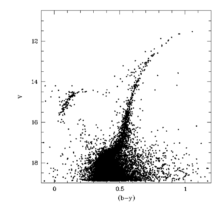
Figure 1: The colour-magnitude diagram of M55. It is cleaned by error cuts ($\sigma_{V}<0.2$ mag)

3 M55

3.1 The colour-magnitude diagram

Fig. 1 shows the CMD of M55. From the original data set of 17269 stars, all objects within an inner radius of 320$\aas@@fstack{\prime\prime}0$ have been taken. We selected according to a maximum error in $V$ of $\sigma_{V}<0.2$ mag for the stars brighter than $V=20.5$. The narrow giant branch and the well defined blue horizontal branch (BHB) show the high internal precision of the selected subsample for the bright stars in M55. Below $V=17.0$ the photometric errors increase quickly and produce the large scatter near the turn-off point.

A number of blue-straggler stars populate the CMD in the region between the horizontal branch and the turn-off point. These objects will be discussed in the appendix.

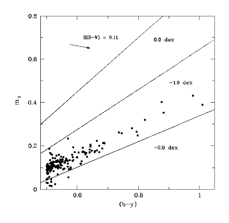
Figure 2: The $m_{1},(b-y)$ diagram of M55 shows a sharp sequence of giant branch stars, in striking contrast to M22, where the distribution is much broader. The diagram has been reddening corrected with $E(B-V)=0.11$. The indicated lines of constant metallicity are taken from the calibration of Hilker (priv. comm.)

3.2 The $m_{1},(b-y)$ diagram

In the $m_{1},(b-y)$ diagram of M55 (Fig. 2) stars with $V<16$ and $(b-y)>0.5$ have been plotted. The $m_{1},(b-y)$ diagram shows a well defined sequence of the giant-branch stars and there is no evidence for a colour spread larger than the photometric errors. The diagram is reddening corrected with $E(B-V)=0.11$. We obtain this value from our photometric data, as we show in the following section.

Through the correlation between [Fe/H], $m_{1}$ and $(b-y)$ the $m_{1},(b-y)$ diagram can be used to derive metallicities for individual giant-branch stars in globular clusters (Grebel & Richtler 1992). A new calibration of the $m_{1},(b-y)$ diagram for the metallicity of red giants is given by Hilker (priv. comm.), in Fig. 2 indicated for the metallicities of $0.0$,$-1.0$ and $-2.0$ dex. It is based on a sample of 60 stars with known Strömgren colours and spectroscopically determined [Fe/H]-values in the range $-2.4$ dex $\leq$ [Fe/H] $\leq$ $-0.6$ dex. 36 stars are taken from the work of Anthony-Twarog & Twarog (1998), 17 from a sample in $\omega$ Centauri and 7 stars of M22 from this work. The metallicity then is given by:

$${\rm[Fe/H]}=\frac{m_{1,0}-1.253\pm 0.062\cdot(b-y)_{0}+0.303\pm 0.046}{0.331\pm 0.045\cdot(b-y)_{0}-0.026\pm 0.033}$$

For stars more metal rich than [Fe/H] = $-0.6$ dex the new calibration has been adjusted to the older one of Grebel & Richtler (1992). Values for [Fe/H] derived by this method are sensitive to the adopted reddening. However, the CMD of a globular cluster also contains information about its reddening and metallicity. Gratton & Ortolani (1989) find the following correlation between [Fe/H] and the colour of the giant branch in globular clusters at the level of the horizontal branch, $(B-V)_{\rm 0,g}$ :

$${\rm[Fe/H]}=2.85\pm 0.37\cdot(B-V)_{\rm 0,g}-3.76\pm 0.31$$

For these two equations reddening and metallicity are correlated in different ways, so that with the combination of both an unambiguous result for [Fe/H] and $E(B-V)$ can be obtained.

For M55 we find $(b-y)_{\rm 0,g}=0.60\pm 0.03$, equivalent to $(B-V)_{\rm 0,g}=0.83\pm 0.06$ (Grebel & Roberts, priv. comm.). Following Hilker’s calibration of the $m_{1},(b-y)$ diagram for stars with $(b-y)\geq 0.6$ we find a reddening of $E(B-V)=0.11\pm 0.02$ and a mean Strömgren metallicity of [Fe/H]$=-1.71\pm 0.04$ dex for M55. This result is, within the error range, in good agreement with the value of Zinn & West (1984; $-1.82\pm 0.15$ dex).

Table 4: CN strengths and Strömgren colours of red giants in M55. The values of $S$(3839) have been taken from Briley et al. (1993)

Nr.Lee	$V$	$(b-y)$	$m_{1}$	$\Delta m_{1}$	$S(3839)$
1317	11.949	0.874	0.232	$-$0.026	0.01
1319	13.089	0.707	0.151	$-$0.005	0.16
1401	12.103	0.856	0.265	$+$0.018	0.20
1404	13.857	0.644	0.116	$-$0.002	0.08
1418	13.042	0.717	0.153	$-$0.010	0.12
1518	11.639	0.953	0.385	$+$0.079	0.10
1523	13.158	0.702	0.153	0.000	0.11
2307	12.628	0.766	0.195	$+$0.002	0.31
2318	12.948	0.725	0.162	$-$0.005	0.19
2437	11.813	0.898	0.303	$+$0.030	0.09
2502	11.653	0.959	0.336	$+$0.026	0.18
2510	13.076	0.701	0.153	0.000	0.21
2517	13.040	0.704	0.144	$-$0.011	0.09
3321	11.988	0.871	0.248	$-$0.007	0.09
3402	13.548	0.601	0.089	$-$0.007	0.07
3409	12.854	0.721	0.180	$+$0.015	0.10
3509	12.247	0.822	0.241	$+$0.014	0.02
3516	13.498	0.661	0.143	$+$0.014	0.20
3519	13.849	0.656	0.084	$-$0.041	0.24
3526	12.860	0.721	0.188	$+$0.023	0.12
4323	12.974	0.734	0.154	$-$0.018	0.20
4403	12.743	0.749	0.154	$-$0.028	0.13
4422	12.394	0.765	0.198	$+$0.006	0.08
4431	13.386	0.669	0.154	$+$0.020	0.22
4501	13.403	0.692	0.113	$-$0.034	0.20
4505	11.532	1.057	0.414	$+$0.045	0.28
4523	12.499	0.741	0.162	$-$0.015	0.26

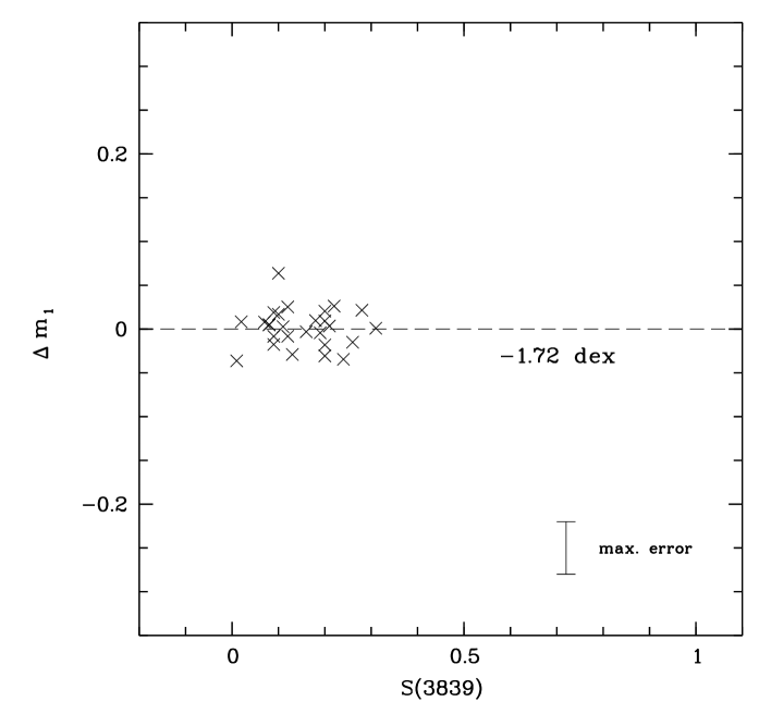
Figure 3: The dispersion of the $m_{1}$ values does not correspond to the CN abundances in M55. The errorbar in the lower right corner indicates the photometric error in $m_{1}$

3.3 CN abundances

Richtler (1988) found (on the basis of aperture photometry) that the giant branch in the M55 $m_{1},(b-y)$ diagram splits up in two sub-branches where the corresponding metallicities anticorrelate with the CN band strengths given by Smith & Norris (1982). Since in other clusters an anticorrelation between C and N is well established (e.g. Suntzeff 1993), the suspicion was that a continous absorption of CO, which affects the Strömgren $v$-filter, could be responsible for this effect.

For comparison, we took 27 stars from the sample of Briley et al. (1993) with known CN abundances (Table 4), identified by the identification numbers from Lee (1976). This sample also includes results from the measurements of Smith & Norris (1982). The range of cyanogen strengths is given by $0.01<S(3839)<0.31$ (Briley et al. 1993), where $S(3839)$ is the spectroscopic index for the CN band beginning at 3883 Å (see Norris & Freeman 1982 for a detailed description). In our $m_{1},(b-y)$ diagram of M55 (Fig. 2) the scatter in $m_{1}$ is small and therefore no signs for significant CN variations are visible. The mean Strömgren metallicity of the selected 27 stars is $-1.72$ dex, derived with the calibration of Hilker. We define $\Delta m_{1}$ to be the vertical distance from the position of an individual star in the $m_{1},(b-y)$ diagram to the calibration line of $-1.72$ dex. In Fig. 3, $\Delta m_{1}$ has been plotted versus the cyanogen index $S(3839)$. No correlation between the $\Delta m_{1}$ values and the cyanogen strengths can be seen. The variations of the $\Delta m_{1}$ values are of similar size as the photometric errors of the $m_{1}$ index, so that the $m_{1}$-CN anticorrelation found by Richtler (1988) might be below our detection limit. However, our measurements give no indication for a significant abundance spread in CN in the cluster giants of M55.

The comparison between the photometric study of Richtler (1988) and the present data reveals only slight differences in the measured Strömgren colours. From a comparison of 7 stars we find that our values of $V$, $(b-y)$ and $m_{1}$ show mean deviations of $\Delta V=+0.018$, $\Delta(b-y)=-0.002$ and $\Delta m_{1}=+0.054$ (in the sense of $\Delta$colour $=$ colour${}_{\rm present\,data}-$colour_Richtler). It is most likely that these shifts reflect the usage of different standard stars (see Richtler 1988). Anyway, the differences are of no importance for the qualitative comparison described above.

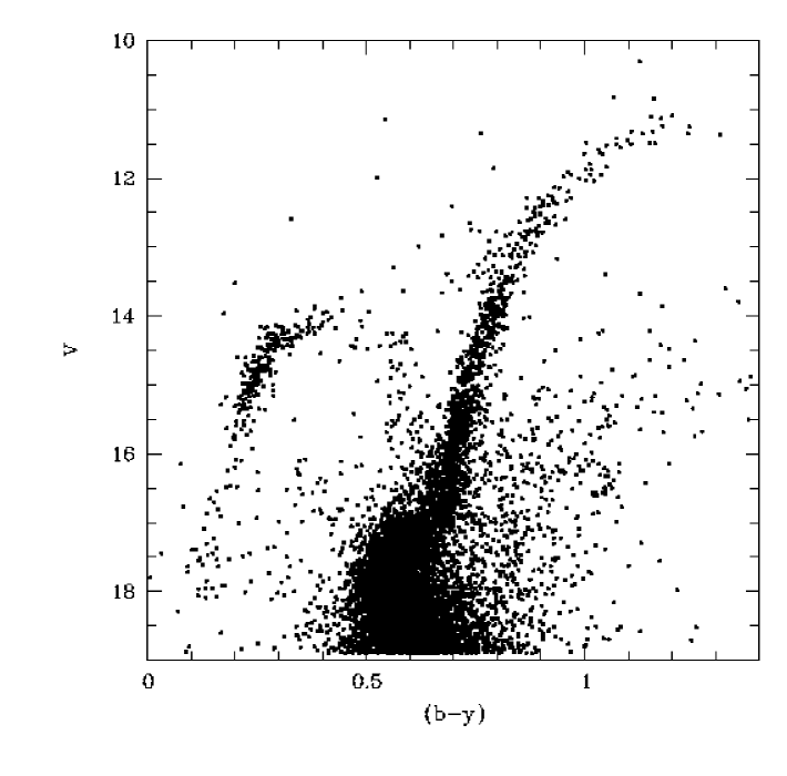
Figure 4: The colour-magnitude diagram of M22 reveals a significant colour dispersion among the red giant branch

4 M22

4.1 The colour-magnitude diagram

The CMD of M22 is presented in Fig. 4. It contains all stars brighter than $V=19.0$ and with $57\aas@@fstack{\prime\prime}0<$ $r$ $<302\aas@@fstack{\prime\prime}0$. The stars from the inner part have been omitted because of the high star density in the center of M22 and the resulting large photometric errors. The shown sample has been cleaned by error selection as done for M55.

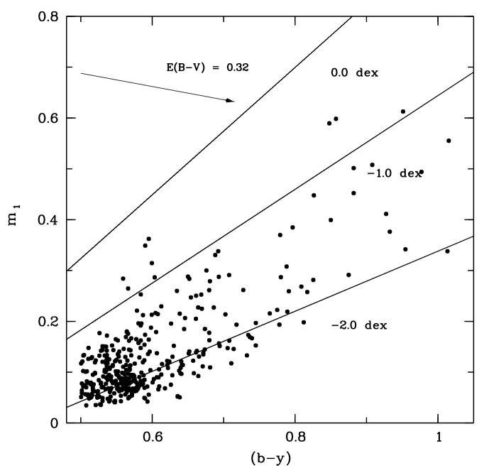
Figure 5: The $m_{1},(b-y)$ diagram of M22 shows a large scatter which can be explained by abundance variations as well as by reddening effects. The diagram has been reddening corrected with $E(B-V)=0.32$, as given by Alcaino & Liller (1983)

The basic features of the red giant branch (RGB) and the blue horizontal branch (BHB) are well defined. In striking difference to M55 is the large colour spread among the red giant branch, as already mentioned by Arp & Melbourne (1959). A similar spread is also visible on the BHB, which suggests that differential reddening is the dominating effect for the origin of the colour dispersion in the CMD. However, since a contribution to the colour range by a possible metallicity spread in M22 can not be excluded, the CMD alone can not clarify the situation.

In the following, we select red giants by defining the ridges of the red giant branch by two parallel curves which at $V=14$ are separated in colour by $0.08$ mag.

4.2 The $m_{1},(b-y)$ diagram

Fig. 5 shows the $m_{1},(b-y)$ diagram of M22. Selected are stars from the red giant branch with $V<16.0$ and $(b-y)>0.5$. In sharp contrast to M55, the distribution of stars does not exhibit a well defined straight line but shows a strongly scattered distribution, so that an accurate determination of a mean cluster metallicity with the method described in Sect. 3.2 is not possible without knowing the reasons for the colour spread.

Previous measurements indicate that the foreground reddening in the direction to M22 is $\geq 0.30$ mag (e.g. Alcaino & Liller 1983, Crocker 1988). In addition, recent spectroscopic studies in M22 lead to a mean cluster metallicity of $-1.48$ dex (Carretta & Gratton 1997). The $m_{1},(b-y)$ diagram shown in Fig. 5 is reddening corrected with $E(B-V)=0.32$, equivalent to the value given by Alcaino & Liller (1983). Using Hilker’s calibration, some of the giant branch stars with $(b-y)\geq 0.6$ lie in a range higher than $-1.2$ dex, so that, with respect to the expected mean metallicity, the giants seem to be scattered to higher metallicities. Since any additional reddening would further increase the metallicity, differential reddening is not a likely candidate in explaining the broad distribution. Moreover, we demonstrate directly that differential reddening does not play a role but that the CN band strengths are responsible.

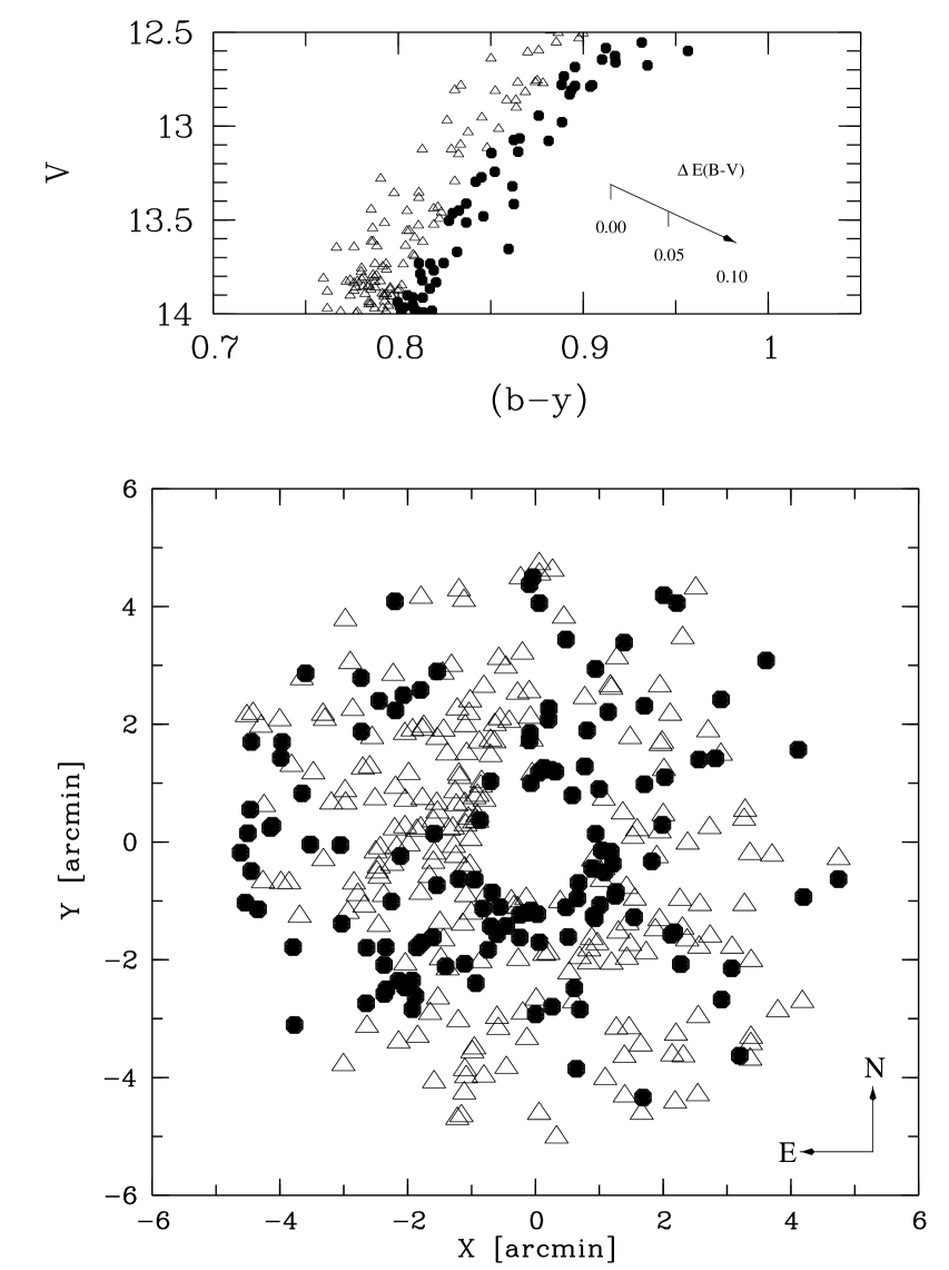
Figure 6: Upper panel: The wide RGB of M22, splitted in the redder giants (filled dots) and the bluer ones (open triangles). Lower panel: The reddest giants are concentrated in a region in the south of the cluster field

Table 5: CN strengths (Norris & Freeman 1982, 1983) and Strömgren colours of red giants in M22

Nr.Arp	$V$	$(b-y)$	$m_{1}$	$\Delta m_{1}$	S(3839)		Nr.Arp	$V$	$(b-y)$	$m_{1}$	$\Delta m_{1}$	$S(3839)$
I8	11.979	0.951	0.212	$+$0.025	0.49		II67	11.253	1.239	0.506	$+$0.141	0.64
I11	12.765	0.874	0.239	$+$0.099	0.54		II77	12.677	0.935	0.068	$-$0.109	0.14
I12	11.640	0.999	0.173	$-$0.044	0.16		II80	11.488	1.149	0.420	$+$0.111	0.85
I36	11.902	0.961	0.120	$-$0.073	0.04		II92	12.555	0.932	0.242	$+$0.067	0.76
I37	11.942	0.969	0.148	$-$0.051	0.16		II98	12.274	0.927	0.164	$-$0.008	0.23
I45	12.504	0.886	0.093	$-$0.055	0.05		II104	12.322	0.959	0.124	$-$0.068	$-$0.01
I51	12.735	0.890	0.081	$-$0.068	$-$0.03		III3	11.130	1.175	0.563	$+$0.238	0.50
I53	12.645	0.910	0.178	$+$0.016	0.54		III6	12.786	0.896	0.086	$-$0.067	0.14
I54	12.770	0.878	0.198	$+$0.055	0.45		III12	11.503	1.106	0.452	$+$0.170	0.58
I57	11.856	0.793	0.344	$+$0.255	0.48		III14	11.096	1.201	0.445	$+$0.104	0.00
I68	12.490	0.882	0.049	$-$0.096	$-$0.05		III15	11.325	1.106	0.403	$+$0.120	0.33
I80	12.506	0.900	0.251	$+$0.095	0.85		III25	12.640	0.850	0.026	$-$0.099	$-$0.14
I85	12.438	0.867	0.065	$-$0.070	0.05		III26	11.111	1.151	0.362	$+$0.051	0.06
I86	12.284	0.969	0.103	$-$0.095	0.05		III35	12.353	0.930	0.098	$-$0.076	0.06
I92	11.522	1.050	0.232	$-$0.016	0.08		III39	12.533	0.898	0.095	$-$0.059	0.24
I98	12.286	0.868	0.089	$-$0.047	0.21		III45	12.818	0.869	0.136	$-$0.001	0.40
I105	12.135	0.932	0.113	$-$0.063	0.18		III47	12.329	0.904	0.128	$-$0.030	0.19
I106	12.431	0.885	0.090	$-$0.057	0.19		III52	11.556	1.081	0.549	$+$0.282	0.55
I108	12.782	0.799	0.018	$-$0.075	$-$0.08		III61	11.791	1.012	0.259	$+$0.034	0.50
I109	12.328	0.904	0.114	$-$0.045	$-$0.04		III86	12.439	0.885	0.156	$+$0.009	0.32
I110	12.757	0.875	0.088	$-$0.053	0.12		IV17	11.356	1.237	0.289	$-$0.075	0.23
I113	12.375	0.938	0.096	$-$0.083	0.29		IV20	12.041	1.021	0.336	$+$0.106	0.72
I116	12.783	0.834	0.023	$-$0.092	0.25		IV24	12.584	0.912	0.281	$+$0.118	0.98
II1	12.032	1.003	0.321	$+$0.101	0.50		IV25	12.842	0.819	0.044	$-$0.062	$-$0.03
II9	12.780	0.888	0.178	$+$0.029	0.58		IV31	12.554	0.885	0.201	$+$0.054	0.68
II23	12.596	0.876	0.092	$-$0.049	0.09		IV59	11.875	1.002	0.144	$-$0.074	0.23
II26	11.326	1.157	0.327	$+$0.013	0.29		IV61	12.599	0.957	0.084	$-$0.107	0.14
II30	12.147	0.942	0.144	$-$0.037	0.12		IV67	12.389	0.905	0.060	$-$0.099	0.03
II31	11.878	1.015	0.210	$-$0.017	0.12		IV73	12.901	0.864	0.059	$-$0.074	$-$0.06
II42	12.767	0.865	0.072	$-$0.062	$-$0.01		IV76	12.257	0.916	0.289	$+$0.123	0.79

Dividing the red giants in a red and a blue sample, as indicated in the upper panel of Fig. 6 by filled dots and open triangles, respectively, provides a simple means to assess the role of differential reddening. The lower panel shows the distribution projected on the sphere. The redder stars clearly tend to be on the southern side, especially along a narrow region from the center towards the south of the cluster. In contrast, many of the bluer giants are located on the north-eastern side. Subdividing the cluster into quarters we find an excess of red stars in the south-eastern quarter with a significance of 2$\sigma$. In contrast, there is a deficiency of red stars (at a 4$\sigma$ level) in the north-eastern quarter (see Fig. 6, lower panel). With regard to the cumulative distribution of red and blue stars in the azimuthal angle we obtain a probability of $\sim 95$ percent that the red and the blue giants are taken from a different distribution function (Kolmogorov-Smirnov test). This inhomogeneous distribution of the red and blue cluster giants indicates variations in the reddening, obviously caused by patchily structured dust in the foreground of M22. From the width of the giant branch (Fig. 6, upper panel) we estimate a total range of $0.07$ mag for the reddening variations, after taking a photometric error in $(b-y)$ of $0.019$ mag into account.

Fig. 7 provides an assessment of the appearance of “red” and “blue” red giants in the $m_{1},(b-y)$ diagram, but no correlation between the scatter in this diagram and the colour spread in the CMD is visible. We would expect that “red” RGB stars show systematically lower metallicities, if reddening would be dominantly responsible for a stellar locus in the $m_{1}$,$(b-y)$ diagram. Variable CN-abundances remain as a plausible explanation for the scatter.

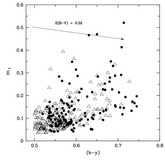
Figure 7: No correlation between the colour of giant branch stars (symbols are from Fig. 6) and the dispersion of $m_{1}$ values can be seen in the $m_{1},(b-y)$ diagram of M22. Therefore reddening variations can not be responsible for the large scatter seen in this diagram

4.3 CN abundances

The strong CN-band at 4216 Å can reduce the flux in the $v$ filter significantly and thus may lead to a higher $m_{1}$ value, while the overall metallicity remains the same (Bell & Gustafsson 1978). The distribution in the $m_{1},(b-y)$ diagram therefore may be an indication that the M22 giants exhibit strongly variing CN-bands. A large range of CN abundances in M22 has indeed been spectroscopically observed by NF.

60 giant stars from the sample of NF with known CN abundances have been identified and compared with our data. Table 5 shows these stars with the identification numbers from Arp & Melbourne (1959), magnitudes and colours from our photometry, and the CN band abundances from NF, given by the index $S(3839)$. Values for the $S(3839)$ index vary between $-0.14$ (CN weak) and $+0.98$ (CN strong) and the CN variations therefore are significantly higher than observed in M55. To investigate the influence of the CN strengths on the $m_{1}$ index in the case of M22, all CN strong stars with $S(3839)$ values larger than $+0.40$ have been plotted in the $m_{1},(b-y)$ diagram (Fig. 8, upper panel) as filled circles, while the CN weak stars ($S(3839)\leq 0.40$) are shown as open circles. The correlation between the positions of the giants in the $m_{1},(b-y)$ diagram and their CN abundances is clearly visible. All stars with strong CN abundances are located in the upper part of the diagram and it is reasonable to conclude that also all the other stars in this area, that have no spectroscopic measurements, are CN rich as well.

The influence of the cyanogen strengths on the $m_{1}$ index can be seen in more detail by using the metallicity calibration for the $m_{1},(b-y)$ diagram. The mean Strömgren metallicity (using the calibration of Hilker) of all 60 giant stars with known CN abundances is $-1.73$ dex, taking a reddening value of $E(B-V)=0.32$ into account (the CN strengths definitely influence this value; it is therefore too high). In Fig. 8 (lower panel), $\Delta m_{1}$ (as defined in Sect. 3.3) to the calibration line of $-1.73$ dex is plotted versus $S(3839)$. In contrast to M55, the influence of the cyanogen strenghts on the $m_{1}$ index in M22 is significant. $\Delta m_{1}$ becomes larger by increasing CN abundances and the CN variations therefore shift the giant stars to higher $m_{1}$ values. This effect dominates the shape of the $m_{1},(b-y)$ diagram, it is even stronger than the reddening variations of about $0.07$ mag. Our results are similar to investigations of Anthony-Twarog et al. (1995), who investigated CN and Ca abundances in relation with the Strömgren $m_{1}$ index for M22. We compared 15 stars from their observations with our data stars and find a good agreement in the measured Strömgren colours. Mean deviations are $\Delta V=-0.029$, $\Delta(b-y)=-0.034$ and $\Delta m_{1}=-0.010$ (see also Sect. 3.3).

The fact that only strong cyanogen abundances influence the $m_{1}$ index offers us the possibility to determine the mean Strömgren metallicity and the mean reddening for M22 using only the 40 spectroscopically measured CN weak giants. With the method described in Sect. 3.2 we derive a cluster metallicity of $-1.62\pm 0.08$ dex and a reddening of $E(B-V)=0.38\pm 0.04$. As for M55, the derived metallicity of M22 is (with regard to the expected errors) in agreement with recent spectroscopic results, such as from Carretta & Gratton (1997, $-1.48\pm 0.06$ dex) and Lehnert et al. (1991, $-1.55\pm 0.11$ dex).

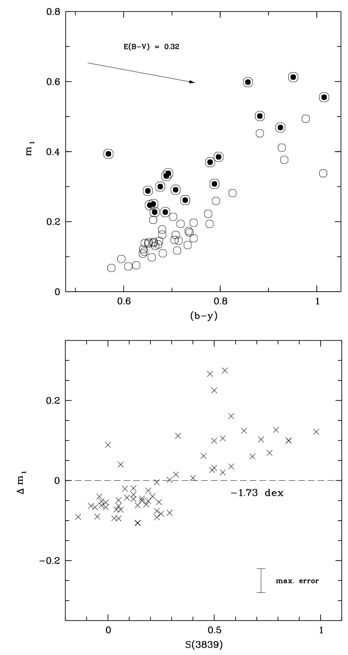
Figure 8: Upper panel: All CN rich stars in M22 show higher $m_{1}$ values than comparable stars with lower CN abundances. Lower panel: The CN abundances are correlated to the vertical distance of the slope which represents the mean Strömgren metallicity for the selected giants in M22 with an adopted reddening of $E(B-V)=0.32$

5 Discussion and conclusions

A comparative study of the two galactic globular clusters M55 and M22 has shown that the Strömgren system can efficiently detect differences in the CN-strength distribution of globular clusters. Moreover, with the method presented in Sect. 3.2 Strömgren photometry can be used for the simultaneous determination of mean metallicities and reddening values in globular clusters.

The present study of M55 and M22 has revealed that the clusters are very different regarding the distribution of Strömgren colours. M55 turns out to be very uniform with respect to Strömgren-metallicities. The sharp red giant branch in the CMD as well as in the $m_{1},(b-y)$ diagram indicates the chemical homogeneity of this globular cluster.

For M22, we confirm the results by Anthony-Twarog et al. (1995). A large scatter in the Strömgren $m_{1}$,$(b-y)$ diagram indicates a large spread in CN strengths among red giants. Therefore, Strömgren colours of M22 stars cannot be interpreted in terms of an overall metallicity, in particular nothing can be said concerning an intrinsic metallicity variation among M22 stars. Moreover, the colour spread of the RGB and the BHB in the colour-magnitude diagram of M22 is not caused by a metallicity variation but probably by patchy reddening variations in the order of $\Delta E(B-V)\approx 0.07$ over the cluster area, because most of the reddest giant-branch stars are spatially concentrated in the southern part of the cluster. This, and the fact that there is no correlation between the dispersions in the CMD and the $m_{1},(b-y)$ diagram, led us to conclude that a spread in [Fe/H], if present, is of minor importance with respect to the CN scatter. Considering similar results for M22 of Anthony-Twarog et al. (1995) and the spectroscopic measurements by Lehnert et al. (1991), $\omega$ Cen remains as the only globular cluster in the Milky Way, where significant evidence exists for a possibly primordial dispersion in [Fe/H].

So far, the existence of a wide range of cyanogen strengths has been shown only in a few globular clusters (see Kraft 1994 for a detailed overview) and their origin can be explained by primordial as well as by evolutionary origin. See to this also the extensive discussion in Anthony-Twarog et al. (1995). Perhaps, CN-rich clusters may be brought into relation with anomalies found in the comparison of integrated spectra of M31 clusters with those of galactic globular clusters. Several authors found (Burstein et al. 1988; Brodie & Huchra 1990) that, at the same metallicity, M31 clusters showed stronger CN-features than galactic clusters. Unfortunately, no work exists measuring integral CN strengths for both M22 and M55.

It is of obvious interest to perform a larger census of the CN-strength distribution among globular-cluster stars. The Strömgren system proved to be an efficient tool for this purpose. At present, it is not possible to investigate the relation of “CN-richness” with any other properties of globular clusters. M55 and M22 are perhaps representatives of two classes of globular clusters regarding their CN-strength distribution. If the CN-strengths in M22 are decoupled from stellar evolution, what else can be the cause? A striking difference between M55 and M22 is their stellar density. M55 is one of the most loosely structured globular clusters while, in contrast, M22 has a quite high density. It is imaginable that encounters or merging of stars can change the CN-surface abundance of red giants. It is therefore of high interest to study a larger sample of globular clusters.

Appendix A Blue stragglers in M55

As mentioned in Sect. 3.1, a population of blue straggler stars (BSS) is visible in the CMD of M55 in the area above the turn-off point. The existence of BSS in M55 and their central concentration has already been shown in detailed analyses by Mandushev et al. (1997) and Zaggia et al. (1998).

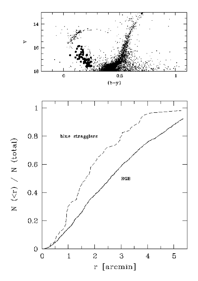
Figure 9: Upper panel: The 56 BSS in the CMD of M55. Lower panel: The cumulative distribution show that the BSS are more centrally concentrated than RGB stars

At present there is much evidence that BSS are close or merged binary stars (e.g. see Mandushev 1997 and references therein). This theory is supported by the finding that the BSS are often more centrally concentrated than other stellar types within globular clusters, which might be indicative for a dynamical mass segregation. In the CMD the BSS sequence ranges up to 2.5 magnitudes above the TOP (see Fig. A1). From our data sample of M55 we selected 56 BSS candidates from the inner $5\aas@@fstack{\prime}3$ for further investigations, shown in Fig. A1 as filled circles.

We compared the spatial distribution of the 56 BSS with that of 1377 sub-giant branch (SGB) stars chosen from the same magnitude interval to ensure that incompleteness does not influence the comparison. In Fig. A1, the cumulative distributions of the SGB stars and the BSS are plotted. The BSS are clearly more concentrated than the SGB stars within the selected radius. Running a Kolmogorov-Smirnov test we obtain a 92 percent probability that the BSS and the SGB stars are taken from different distributions, a value that is similar to the one found by Mandushev et al. (1997) for M55. These results favour mass segregation and further support that BSS have on the average larger masses than subgiants and thus are merged stars or binaries.

References

- (1) Alcaino G., Liller W., 1983, AJ 88, 1330
- (2) Anthony-Twarog B.J., Twarog B.A., 1998, AJ 116, 1922
- (3) Anthony-Twarog B.J., Twarog B.A., Craig J., 1995, PASP 107, 32
- (4) Arp H.C., Melbourne, W.G., 1959, AJ 64, 28
- (5) Bates B., Montgomery A.S., Wood K.D., Davies R.D., Walker H.J., 1992
- (6) Bell R.A., Gustafsson B., 1978, A&AS 34, 229
- (7) Briley M.M., Hesser J.E., Bell R.A., 1991, ApJ 373, 482
- (8) Briley M.M., Smith G.H., Hesser J.E., Bell R.A., 1993, AJ 106, 142
- (9) Brodie J.P., Huchra J.P. 1990, ApJ 362, 503
- (10) Brown J.A., Wallerstein G., 1992, AJ 104, 1818
- (11) Brown J.A., Wallerstein G., Oke J.B., 1990, AJ 100, 1561
- (12) Burstein D., Bertola F., Buson L.M., Faber S.M., Lauer T.R. 1988, ApJ 328, 440
- (13) Carretta E., Gratton R.G., 1997, A&AS 121, 95
- (14) Crocker D.A., 1988, AJ 96, 1649
- (15) Gratton R.G., Ortolani S., 1989, A&A 211, 41
- (16) Grebel E.K., Richtler T., 1992, A&A 253, 359
- (17) Hesser, J.E. 1976, PASP 88, 849
- (18) Hesser J.E., Hartwick F.D.A., McClure R.D., 1977, ApJS 33, 471
- (19) Icke V., Alcaino G., 1988, A&A 204, 115
- (20) Jønch-Sørensen H., 1993, A&AS 102, 637
- (21) Jønch-Sørensen H., 1994, A&AS 108, 403
- (22) Kraft R.P., 1994, PASP 106, 553
- (23) Lee S.-W., 1976, A&AS 29, 1
- (24) Lehnert M.D., Bell R.A., Cohen J.G., 1991, ApJ 367, 514
- (25) Lloyd Evans T., 1978, MNRAS 182, 293
- (26) Mandushev G.I., Fahlman G.G., Richer H.B., 1997, AJ 114, 1060
- (27) Minniti D., Coyne G.V., Tapia S., 1990, A&A 236, 371
- (28) Minniti D., Coyne G.V., Claria J.J., 1992, AJ 103, 871
- (29) Norris J., Freeman K.C., 1982, ApJ 266, 130
- (30) Norris J., Freeman K.C., 1983, ApJ 273, 838
- (31) Norris J.E., Freeman K.C., Mighell K.J., 1996, ApJ 462, 241
- (32) Norris J.E., Freeman K.C., Mayor M., Seitzer P., 1997, ApJ 487, L187
- (33) Persson S.E., Frogel J.A., Cohen J.G., Aaronson M., Matthews K., 1980, ApJ 235, 452
- (34) Peterson R.C., Cudworth K.M., 1994, ApJ 420, 612
- (35) Richtler T., 1988, A&A 204, 101
- (36) Searle L., 1977, In: Tinsley B.M., Larson R.B. (eds.) The Evolution of Galaxies and Stellar Populations, New Haven: Yale Univ. Obs., p. 219
- (37) Smith G.H., Norris J., 1982, ApJ 254, 149
- (38) Stetson P.B., 1987, PASP 99, 191
- (39) Stetson P.B., 1992, In: D.M. Worrall, C. Biemesderfer, J. Barnes (eds.) ASP Conf. Series, Vol. 25, Astronomical Data Analysis Software and Systems, p. 297
- (40) Stryker L.L., 1993, PASP 105, 1081
- (41) Suntzeff N., 1993, In: Smith G.H., Brodie J.P. (eds.) ASP Conf. Series, Vol. 48, The Globular Cluster-Galaxy Connection, p. 167
- (42) Suntzeff N.B., 1989, In: Spite M., Lloyd Evans T. (eds.) The Abundance Spread within Globular Clusters, Obs. de Paris, p. 71
- (43) Zaggia S.R., Piotto G., Capaccioli M., 1998, A&A 327, 1004
- (44) Zinn R., West M.J., 1984, ApJS 55, 45