SPH simulations of magnetic fields in galaxy clusters

Abstract

We perform cosmological, hydrodynamic simulations of magnetic fields in galaxy clusters. The computational code combines the special-purpose hardware Grape for calculating gravitational interaction, and smooth-particle hydrodynamics for the gas component. We employ the usual MHD equations for the evolution of the magnetic field in an ideally conducting plasma. As a first application, we focus on the question what kind of initial magnetic fields yield final field configurations within clusters which are compatible with Faraday-rotation measurements. Our main results can be summarised as follows: (i) Initial magnetic field strengths are amplified by approximately three orders of magnitude in cluster cores, one order of magnitude above the expectation from spherical collapse. (ii) Vastly different initial field configurations (homogeneous or chaotic) yield results that cannot significantly be distinguished. (iii) Micro-Gauss fields and Faraday-rotation observations are well reproduced in our simulations starting from initial magnetic fields of $\sim 10^{-9}\,{\rm G}$ strength. Our results show that (i) shear flows in clusters are crucial for amplifying magnetic fields beyond simple compression, (ii) final field configurations in clusters are dominated by the cluster collapse rather than by the initial configuration, and (iii) initial magnetic fields of order $10^{-9}\,{\rm G}$ are required to match Faraday-rotation observations in real clusters.

1 Introduction

Magnetic fields in galaxy clusters are inferred from observations of diffuse radio haloes (Kronberg 1994) and Faraday rotation (Vallee, MacLeod & Broten 1986, 1987).

It is therefore evident that clusters of galaxies are pervaded by magnetic fields of $\sim\mu{\rm G}$ strength.

Various models have been proposed for the origin of cluster magnetic fields in individual galaxies (Rephaeli 1988; Ruzmaikin, Sokolov & Shukurov 1989). The basic argument behind such models is that the metal abundances in the intra-cluster plasma are comparable to solar values. The plasma therefore must have been substantially enriched by galactic winds which could at the same time have blown the galactic magnetic fields into intra-cluster space.

We here address the question whether seed magnetic fields of speculative origin, magnified in the collapse of cosmic material into galaxy clusters, can reproduce a number of observations, particularly Faraday-rotation measurements. Specifically, we ask what initial conditions we must require for the seed fields in order to reproduce the statistics of rotation-measure observations. A compilation of available observations of this kind was published by Kim, Kronberg & Tribble (1991).

2 GrapeMSPH

We start with the GrapeSPH code developed and kindly provided by Matthias Steinmetz (Steinmetz 1996). It simultaneously computes with a multiple time-step scheme the behaviour of two matter components, a dissipation-free dark matter component interacting only through gravity, and a dissipational, gaseous component. The gravitational interaction is evaluated on the Grape board, while the hydrodynamics is calculated by the CPU of the host work-station in the smooth-particle approach (SPH, Lucy 1977; Monaghan 1985). We supplement the code with the magneto-hydrodynamic equations to follow the evolution of an initial magnetic field caused by the flow of the gaseous matter component. Details on GrapeMSPH and on the results can be found in Dolag, Bartelmann & Lesch (1999). Fig. 1 shows the appearance of a typical simulation at the end of a calculation.

3 Initial conditions

We need two types of initial conditions, namely (i) the cosmological parameters and initial density perturbations, and (ii) the properties of the primordial magnetic field. For the purposes of the present study, we set up cosmological initial conditions in an Einstein-de Sitter universe ($\Omega^{0}_{\rm m}=1$, $\Omega^{0}_{\rm\Lambda}=0$) with a Hubble constant of $H_{0}=50\,{\rm km\,s^{-1}\,Mpc^{-1}}$. We initialise density fluctuations according to a COBE-normalised CDM power spectrum. The origin of the observed cluster magnetic fields is uncertain. We therefore use two extreme set-ups for the initial magnetic field, namely either a chaotic or a completely homogeneous magnetic field at high redshift ($z=15$). For a fair comparison we fixed the average magnetic field energy density to the same value in both cases.

4 Results

The magnetic field in our simulated clusters is dynamically unimportant even in the densest regions, i.e. the cluster cores. Since we ignore cooling, this result may change close to cluster centres where cooling can become efficient and cooling flows can form.

Magnetic flux conservation in an ideally conducting plasma leads to an enhancement of the magnetic field during spherically symmetric cluster collapse proportional to $\rho^{2/3}$, where $\rho$ is the gas density. An initial intracluster field of order $10^{-9}\,{\rm G}$ is therefore expected to be magnified only up to $10^{-7}\,{\rm G}$. Our simulations, however, demonstrate that such seed fields can be magnified up to $10^{-6}\,{\rm G}$ in final stages of cluster evolution. Shear flows therefore stretch and tangle the magnetic field, leading to an extra amount of amplification during the cluster formation process.

4.1 Different initial field set-ups

In order to evaluate what the two different kinds of initial magnetic-field set-ups imply for the observations of rotation measures (Fig. 2), we compute rotation-measure maps from the cluster simulations (lower part of Fig. 1) and compare them statistically. We use two methods for that. First is the usual Kolmogorov-Smirnov test, which evaluates the probability with which two sets of data can have been drawn from the same parent distribution. Second is an excursion-set approach, in which we compute the fraction ${\cal F}$ of the total cluster surface covered by RM values exceeding a certain threshold. For the cluster surface area, we take the area of the region emitting 90% of the X-ray luminosity.

Fig. 4 shows how the RM distributions evolve in clusters in which the initial magnetic field was set up either homogeneously or chaotically. We use the excursion-set approach here, i.e. we plot the fraction ${\cal F}$ of the cluster area that is covered by regions in which the RM exceeds a certain threshold.

Quite generally, this fractional area for fixed RM threshold increases during the process of cluster formation. As Fig. 4 shows, the difference between initially homogeneous (heavy lines) and chaotic (thin lines) magnetic fields is negligible.

4.2 Individual cluster

We can now compare the simulated RM statistics with measurements in individual clusters like Coma, for which a fair number of measurements is available, as done in Fig. 3. The distribution of the RM values as a function of distance to the cluster centre are shown for the Coma cluster as points in the lower right panel. The cumulative distribution of these measurements (dash-dotted curve) is shown in the upper panel. This distribution can now be compared to the RM values obtained from the simulations (other lines in all panels). We choosed random beam positions under the constraint that their radial distribution match the observed one. In this example, the Kolmogorov-Smirnov likelihood for 30 simulated beams to match the ten measurements in Coma falls between 30% and 50% for the less massive cluster (solid and dashed curves), compared to a few per cent for the more massive one (dotted curve). Since the less massive cluster has approximately the estimated mass of Coma, this demonstrates that our simulations well reproduce the RM measurements in Coma.

4.3 A sample of clusters

Unfortunately, in most clusters the number of radio sources suitable for measurements of Faraday rotation is only one or two. We therefore also compare a sample of simulated clusters with a compilation of RM observations in different clusters. Fig. 5 shows the values published by Kim et al. (1991). We take the absolute RM value and plot it against the distance to the nearest Abell cluster in units of the estimated Abell radius (crosses).

The increase of the signal towards the cluster centres is evident. In order not to be dominated by a few outliers, which in some cases even fall outside the plotted region and are marked by the arrows at the top of the plot, we did not calculate mean and variance, but rather the median and the $25$- and $75$-percentiles of the RM distribution (solid curves).

The median of synthetic radial rotation-measure distributions obtained from our simulations for different initial magnetic field strengths is shown by the dashed and dotted curves. The initial magnetic field strengths are $10^{-9}{\rm G}$ and $0.2\times 10^{-9}{\rm G}$ as indicated in the figure. An initial field strength of order $\approx 10^{-9}\,{\rm G}$ at redshift $15$ reasonably reproduces the observations.

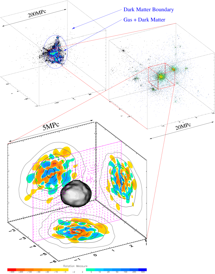
Figure 1: Our simulations work with three classes of particles. In a central region, we have $\sim 50,000$ collision-less dark-matter particles with mass $3.2\times 10^{11}\,M_{\odot}$, mixed with an equal number of gas particles whose mass is twenty times smaller. These gas particles carry the magnetic field. The central region is surrounded by $\sim 20,000$ collision-less boundary particles whose mass increases outward to mimic the tidal forces of the neighbouring large scale structure. The figure shows the structure of this kind of simulation at redshift $z=0$ from the whole simulated volume down to the cluster. The lower box in this figure shows one simulated cluster in a three-dimensional box and also appears as color print. The Faraday-rotation measures produced by the cluster in the three independent spatial directions are projected onto the box sides and encoded by the color-scale as indicated below the box. The gray solid curves are projected density contours, whereas the dashed line marks half the central density. The green dashed curve encompasses the region emitting 90% of the projected X-ray luminosity. The shaded object in the center is the isodensity surface at hundred times the critical density. In addition, magnetic field vectors are plotted in the slice marked by the purple rectangle. Coordinates are physical coordinates in Mpc.

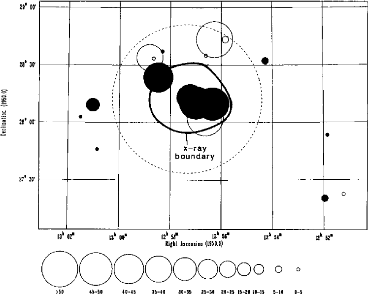
Figure 2: Values and positions of rotation measures observed in the Coma cluster (reproduced from Kim et al. 1990).

Figure 3: This figure shows different visualizations of the RM statistics for a simulated cluster. Shown are a Cluster with homogeneous (solid line) and chaotic (dashed line) initial magnetic field, an approximately twice as massive cluster (dotted line), and observations in the Coma cluster (dashed-dotted line or points). The top panel shows cumulative distributions of rotation measures. A Kolmogorov-Smirnov test reveals a thirty percent chance for the observations to be drawn from the simulated distributions for the smaller and only one per cent for the more massive cluster, whereas the homogeneous and chaotic initial conditions cannot be distinguished. The additional plot in the upper panel shows the final comparison with the Coma measurements, applying some corrections for intrinsic Faraday rotation and spatial distribution of the sources. The lower left panel shows the distribution of the RM measurements inside the X-Ray boundary. The more massive cluster has relatively more high and fewer low RM values than the less massive one. The lower right panel shows the mean of the absolute value for the RM measurements as function of the distance to the cluster center. Towards its center, the more massive cluster has higher RM values than Coma, while the less massive one almost reproduces the observations. In the outer parts, both clusters produce somewhat too small RMs.

Figure 4: This figure shows the fraction ${\cal F}$ of the cluster area which is covered by regions in which the absolute value of the rotation measure exceeds a certain threshold for homogeneous (thick line) and chaotic (thin line) initial magnetic fields. The cluster area is taken to be the area of the region emitting 90% of the X-ray luminosity. The results are averaged over the three independent spatial directions. Line types distinguish different RM thresholds, as indicated in the figure.

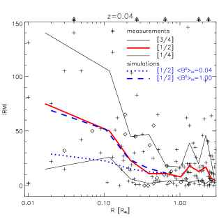
Figure 5: Comparison of simulated results with a sample of measurements in Abell clusters. The absolute values of Faraday rotation measurements (Kim et al. 1991) vs. radius in units of the Abell radius are shown. Obviously, the dispersion increases towards the cluster center. The solid curves mark the median and the 25- and 75-percentiles of the measurements, and the dashed and dotted curves are the medians obtained from simulated cluster samples starting with high and low magnetic fields as marked in the plot, respectively. The radial bins are chosen such as to contain 15 data points each. The scatter in the observations is large, but the simulations with the stronger initial magnetic field seem to match the observations better.

References

- [1] Dolag, K., Bartelmann, M., Lesch, H., 1999, A&A, in press
- [2] Kim, K.T., Kronberg, P.P., Dewdney, P.E., Landecker, T.L., 1990, ApJ, 355, 29
- [3] Kim, K.T., Kronberg, P.P., Tribble, P.C., 1991, ApJ, 379, 80
- [4] Kronberg, P.P., 1994, Rep. Prog. Phys., 57, 325
- [5] Lucy, L., 1977, AJ, 82, 1013
- [6] Monaghan, J.J., 1985, J. Comput. Phys., 3, 71
- [7] Rephaeli, Y., 1988, ComAp, 12, 265
- [8] Ruzmaikin, A., Sokolov, D., Shukurov, A.,1989,MNRAS,241,1
- [9] Steinmetz, M., 1996, MNRAS, 278, 1005
- [10] Vallee, J.P., MacLeod, J.M., Broten, N.W., 1986, A&A, 156, 386
- [11] Vallee, J.P., MacLeod, J.M., Broten, N.W., 1987, ApL, 25, 181