INHOMOGENEOUS REIONIZATION REGULATED BY RADIATIVE AND STELLAR FEEDBACKS

Abstract

We study the inhomogeneous reionization in a critical density CDM universe due to stellar sources, including Population III objects. The spatial distribution of the sources is obtained from high resolution numerical N-body simulations. We calculate the source properties taking into account a self-consistent treatment of both radiative (i.e. ionizing and H₂ -photodissociating photons) and stellar (i.e. SN explosions) feedbacks regulated by massive stars. This allows us to describe the topology of the ionized and dissociated regions at various cosmic epochs and derive the evolution of H, He, and H₂ filling factors, soft UV background, cosmic star formation rate and the final fate of ionizing objects. The main results are: (i) galaxies reionize the IGM by $z$$\approx$10 (with some uncertainty related to the gas clumping factor), whereas H₂ is completely dissociated already by $z$$\approx$25; (ii) reionization is mostly due to the relatively massive objects which collapse via H line cooling, while objects whose formation relies on H₂ cooling alone are insufficient to this aim; (iii) the diffuse soft UV background is the major source of radiative feedback effects for $z\leq 15$; at higher $z$ direct flux from neighboring objects dominates; (iv) the match of the calculated cosmic star formation history with the one observed at lower redshifts suggests that the conversion efficiency of baryons into stars is $\approx$1%; (v) we find that a very large population of dark objects which failed to form stars is present by $z$$\approx$8. We discuss and compare our results with similar previous studies.

1. INTRODUCTION

At $z$$\approx$1100 the intergalactic medium (IGM) is expected to recombine and remain neutral until the first sources of ionizing radiation form and reionize it. The application of the Gunn-Peterson (1965) test to QSOs absorption spectra suggests that the HI reionization is complete by $z$$\approx$5. Recently, Ly$\alpha$ emitters have been seen up to a redshift of $z$=6.68 (Chen, Lanzetta & Pascarelle 1999). This indicates that the IGM was already ionized by then, but the epoch of complete reionization has yet to be firmly established. Several authors (Shapiro, Giroux & Babul 1994; Madau, Haardt & Rees 1998 and references therein) have claimed that the known population of quasars (showing a pronounced cutoff at $z\lower 2.15277pt\hbox{$\;\buildrel>\over{\sim}\;$}3$ [Warren, Hewett & Osmer 1994; Schmidt, Schneider & Gunn 1995; Shaver et al. 1996]) and galaxies provides $\approx$10 times fewer ionizing photons than are necessary to keep the observed IGM ionization level. Thus, additional sources of ionizing photons are required at high redshift. Although models have been proposed in which the UV photons responsible for the IGM reionization may be emitted by a cosmological distribution of decaying dark matter particles, such as neutrinos (see for example Scott, Rees & Sciama 1991), the most promising sources are early galaxies and quasars.

Recent observational evidence suggest the existence of an early population of pregalactic objects which could have contributed to the reionization and metal enrichment of the IGM. Metals have been clearly detected in Ly$\alpha$ forest clouds with column densities low enough to be identified with a truly diffuse IGM (Cowie et al. 1995; Tytler et al. 1995; Lu et al. 1998; Cowie & Songaila 1998), although discrepant metallicities have been inferred. Naively, one can estimate that the amount of heavy elements associated with the number of photons required to ionize every baryon in the universe a few times corresponds to an IGM metallicity $Z\approx 3\times 10^{-3}Z_{\odot}$. This figure is roughly consistent with the value obtained by Cowie & Songaila (1998), but ten times larger than the one derived by Lu et al. (1998). The reasons for this discrepancy are not yet clear. Whatever the correct level of metallicity is, these heavy elements must have been produced by objects hosting the sites of the earliest star formation activity in the universe. The presence of a soft, stellar component of the UV background deduced from studies of the [Si/C] abundance ratios in low column density absorption systems (Savaglio et al. 1997; Giroux & Shull 1997), also supports this view. The question remains concerning the transport mechanism from the production regions, which are presumably associated with high peaks of the density fluctuation field, into the very diffuse medium probed by absorption line experiments. It is currently unclear if the mechanical energy input associated with the same massive stars producing the metals (i.e. supernovae) is sufficient to drive the metals far enough from their production site or if additional mechanisms need be invoked. Although recently Gnedin (1998), using high resolution cosmological simulations which include a coarse modelling of a two-phase interstellar medium, has suggested that merging is the dominant mechanism for transporting heavy elements from primeval galaxies into the IGM, direct ejection of the metal enriched interstellar gas by supernovae or stellar winds may still play an important role.

A contribution to the ionizing flux at high redshift from an early population of quasars may provide the hard component required for HeII reionization. High resolution spectra of a quasar at $z$$\approx$3 have shown large fluctuations of the HI to HeII optical depth ratio (Reimers et al. 1997), interpreted as evidence for a patchy HeII ionization in the IGM. However, it is unclear if these fluctuations could be rather caused by statistical fluctuations of the IGM density or of the ionizing background flux (Miralda-Escudé 1998; Miralda-Escudé, Haehnelt & Rees 1998). Analytical results from Haiman & Loeb (1998b) show that HeII reionization due to sources with quasar-like spectra should occur at approximately the same redshift as hydrogen reionization; if the predicted HeII reionization redshift will be confirmed by future measurements, this would severely constrain the number of high redshift quasars predicted by theory.

The study of the IGM reionization due to these primeval sources has been tackled by several authors, both via semi-analytical (Shapiro 1986; Fukugita & Kawasaki 1994; Tegmark, Silk & Blanchard 1994; Haiman & Loeb 1998b; Miralda-Escudé, Haehnelt & Rees 1998; Valageas & Silk 1999, VS) and numerical (Gnedin & Ostriker 1997, GO; Norman, Paschos & Abel 1998; Razoumov & Scott 1998) approaches. One of the main difficulties of the problem is the treatment of cosmological radiative transfer. Only recently have numerical approaches have been attempted (Abel, Norman & Madau 1998; Norman, Paschos & Abel 1998), and these still require severe approximations to the radiative transfer equation. Clearly, a numerical approach offers the advantage of a more detailed treatment of features such as the IGM clumpiness (GO; Shapiro, Raga & Mellema 1998), or the source spatial distribution. Conversely, semi-analytical approaches are more flexible and allow a more thorough exploration of the parameter space.

A proper treatment of the reionization problem must take into account the interplay of galaxy formation with the reionization process itself. Basically, two types of feedback, radiative and stellar, can be at work. In the standard cosmological hierarchical scenario for structure formation, the objects which form first are predicted to have masses corresponding to virial temperatures $T_{vir}<10^{4}$ K. Once the gas has virialized in the potential wells of dark matter halos, additional cooling is required to further collapse the gas and form stars. For a gas of primordial composition at such low temperatures the main coolant is molecular hydrogen (Peebles & Dicke 1968; Shapiro 1992; Haiman, Rees & Loeb 1996; Abel et al. 1997a; Tegmark et al. 1997; Ferrara 1998). We define Pop III objects as those for which H₂ cooling is required for collapse. After a H₂ molecule gets rotationally or vibrationally excited through a collision with an H atom or another H₂ molecule, a radiative de-excitation leads to cooling of the gas. This mechanism has been studied in great detail by several authors (Lepp & Shull 1984; Hollenbach & McKee 1989; Martin, Schwarz & Mandy 1996; Galli & Palla 1998) and has been applied to the study of the formation of primordial small mass objects (Haiman, Thoul & Loeb 1996; Tegmark et al. 1997; Abel et al. 1997b). Primordial H₂ forms with a fractional abundance of $\approx 10^{-7}$ at redshifts $\lower 2.15277pt\hbox{$\;\buildrel>\over{\sim}\;$}400$ via the H${}_{2}^{+}$ formation channel. At redshifts $\lower 2.15277pt\hbox{$\;\buildrel<\over{\sim}\;$}110$, when the Cosmic Microwave Background radiation (CMB) intensity becomes weak enough to allow for significant formation of H^- ions, a primordial fraction of $f_{H_{2}}\approx 2\times 10^{-6}$ (Shapiro 1992; Anninos & Norman 1996) is produced for model universes that satisfy the standard primordial nucleosynthesis constrain $\Omega_{b}h^{2}=0.0125$ (Copi, Schramm & Turner 1995), where $\Omega_{b}$ is the baryon density parameter and $H_{0}=100h$ km s^-1 Mpc^-1 is the Hubble constant. This primordial fraction is usually lower than the one required for the formation of Pop III objects, but during the collapse phase, the molecular hydrogen content can reach high enough values to trigger star formation. On the other hand, objects with virial temperatures (or masses) above that required for the hydrogen Ly$\alpha$ line cooling to be efficient, do not rely on H₂ cooling to ignite internal star formation. As the first stars form, their photons in the energy range 11.26-13.6 eV are able to penetrate the gas and photodissociate H₂ molecules both in the IGM and in the nearest collapsing structures, if they can propagate that far from their source. Thus, the existence of a UV flux below the Lyman limit due to primordial objects, capable of dissociating the H₂, could strongly influence subsequent small structure formation. Haiman, Rees & Loeb (1997, HRL), for example, have argued that Pop III objects could depress the H₂ abundance in neighbor collapsing clouds, due to their UV photodissociating radiation, thus inhibiting subsequent formation of small mass structures. On the other hand, Ciardi, Ferrara & Abel (1999, CFA) have shown that the “soft-UV background” (SUVB) produced by Pop IIIs is well below the threshold required for negative feedback to be effective earlier than $z$$\approx$20. In principle, the collapse of larger mass objects can also be influenced by an ionizing background, as gas in halos with a circular velocity lower than the sound speed of ionized gas may be prevented from collapsing due to pressure support in the gravitational potential. Thoul & Weinberg (1996) (see also Babul & Rees 1992) have however shown that the collapse is only delayed by this process. We will refer to this complex network of processes as “radiative feedback”.

The other feedback mechanism is related to massive stars and for this reason we will call it “stellar feedback”. Once star formation begins in the central regions of collapsed objects it may strongly influence their evolution via the effects of mass and energy deposition due to massive stars through winds and supernova explosions. These processes may induce two essentially different phenomena. Low mass objects are characterized by shallow potential wells in which the baryons are only loosely bound and a relatively small energy injection may be sufficient to expel the entire gas content back into the IGM, i.e. a blowaway, thus quenching star formation. Larger objects, may instead be able to at least partially retain their baryons, although a substantial fraction of the latter are lost in an outflow, i.e. a blowout (Ciardi & Ferrara 1997; Mac Low & Ferrara 1999, MF; Ferrara & Tolstoy 1999, FT). However, even in this case the outflow induces a decrease of the star formation rate due to the global heating and loss of the galactic ISM. Omukai & Nishi (1999) have pointed out that the ionizing radiation of the first stars formed in Pop III objects can also produce an abrupt interruption of the star formation by dissociating the internal H₂ content. The effect of this feedback is very similar to the blowaway, as both processes are regulated by massive stars.

Our aim here is to study and describe in detail the reionization process of the IGM. As the ionizing sources are not spatially homogeneously distributed, the pattern of the ionized regions is not uniform, i.e. inhomogeneous reionization takes place. Thus, a crucial ingredient of such calculations is the realistic description of the ionized region topology in the universe. This can be achieved only by numerical simulations which track the formation and merging of dark matter halos. For our purposes, these simulations must reach the highest possible mass resolution in order to unambiguously identify the very small Pop III objects initiating the reionization process. The second fundamental ingredient is a proper treatment of radiative and stellar feedback processes on which a great deal of previous work, either by ourselves or other groups, has been accumulating ranging from semi-analytical studies, to numerical models and hydrodynamical simulations, particularly with regard to stellar feedback. Improving on such results we have been able to effectively model and include in the computations a wide number of effects governed by ionizing/dissociating radiation and massive star energy injection which will be presented and discussed in detail. The delicate link between the properties of dark matter halos, which can be reliably derived from N-body simulations, and those describing their baryonic counterparts is represented by the prescription used to model star formation. The advantages that the proposed approach brings along should become evident by reading the paper: it allows to derive self-consistent inhomogeneous reionization models and to infer the properties of the early galaxies producing it. In addition, its predictive power allows to design specific tests that could validate the results.

The plan of the paper is the following. In §2 we present the N-body numerical simulations and in §3 we describe our assumptions about star formation. Then we turn to the discussion of radiative (§4) and stellar (§5) feedbacks and a brief sketch summarizing the possible galactic evolutionary tracks due to such processes is presented in §6. Results are given in §7 and further discussed in §9. A short summary concludes the paper.

2. NUMERICAL SIMULATIONS AND HALO SELECTION

We have simulated structure formation within a periodic cube of comoving length $L=2.55h^{-1}$ Mpc for a critical density cold dark matter model ($\Omega_{0}$=1, $h$=0.5 with $\sigma_{8}$=0.6 at $z$=0). Our choice for the normalization ($\sigma_{8}$) corresponds roughly to those inferred from the present-day cluster abundance (see, e.g., Eke, Cole & Frenk 1996 and Governato et al. 1999). We remind the reader that once the present-day value of $\sigma_{8}$ for the SCDM run is selected, the redshift epoch of all other outputs with lower values of $\sigma_{8}$ is uniquely specified. For example, for the case where the present-day normalization is chosen to be $\sigma_{8}$=0.6, $\sigma_{8}$=0.3 output corresponds to the $z=1$ epoch. It is useful to note that the rms linear overdensity of a sphere with a mass equal to the box is 2.1/(1+z). At early times when the amplitude of fluctuations are small for scales larger than the box size the simulation box should be large enough to be representative of the world model as a whole. But as the scale of non-linear fluctuations grows there will come a time when the simulation volume will not be large enough to provide a proper average. By redshift 8, for example, the rms linear overdensity of a sphere with the mass of the entire simulation is 0.23 and by then the mass spectrum of dark halos in the simulation box may not match the real mass spectrum very well – particularly at the high mass end.

The initial conditions for the simulations, were set up at $z$=100 and integrated in time to $z$=8.3 (with intermediate outputs at $z$=29.6, 25.3, 22.1, 19.8, 18.0, 16.5, 15.4, 14.3, 11.4 and 10.9). We used a transfer function for CDM calculated with CMBFAST and a baryonic fraction $\Omega_{b}$=0.06 (Copi, Schramm & Turner 1995). The simulation, which uses 256³ particles (about $17$ million), was computed with AP3M (Pearce & Couchman 1997), a parallel P3M code. A cubic spline force softening of 0.05 kpc $h^{-1}$ Plummer equivalent was used so that the overall structure of the halos could be resolved. The good mass (particle mass is $\approx 5\times 10^{5}M_{\odot}$) and force resolution allows us to study in detail the evolution of all structures likely to host the formation of primordial stars.

In numerical simulations, halos can be identified using a variety of schemes. Of these, we have chosen one that is available in the public domain: FOF (Davis et al. 1985). In this scheme, all particle pairs separated by less than $b$ times the mean interparticle separation are linked together. Sets of mutually linked particles form groups that are then identified as dark matter halos. Other halo finders that are often used in literature to find virialized halos are HOP (Eisenstein & Hut 1998), the “spherical overdensity algorithm ” or SO, that finds spherically averaged halos above a given overdensity (Lacey & Cole 1994) and the scheme recently developed by Gross et al. (1998). In the present study, we adopted the linking length that Lacey & Cole (1994) deduced to identify virialized halos with mean densities of $\approx$200 times the critical density at the epoch under consideration. Halo masses (and ultimately, our findings) do not depend on the halo finder used (FOF, HOP or SO), as long as it selects halos including all particles down to the same overdensity. Systematic deviations between different algorithms are of the order of a few per cent (see Governato et al. 1999, Lacey & Cole 1994). In our analysis, we only consider halos consisting of 16 particles or more, corresponding to a mass of $8\times 10^{6}\,M_{\odot}$.

We have compared the results of the numerical simulations for the dark matter halo distribution, with the one obtained from the Press & Schechter (1974, PS) formalism, so that we can use this semi–analytical expression to calculate certain quantities, such as the soft-UV background (see § 4.2). The power spectrum normalization is $\sigma_{8}$=0.6, consistent with the above numerical simulations. Although PS slightly overestimates the halo number density, the match is remarkably good over the entire range of redshifts considered.

Finally, the correlation function for galaxies at high redshift has been recently predicted (Governato et al. 1998) and then measured by Giavalisco et al. (1998), giving strong support to hierarchical models of galaxy formation. Bright galaxies at high redshift form on top of the highest peaks in the mass distribution, and so they are strongly biased with respect to the underlying dark matter distribution. In hierarchical models we expect a similar behavior for the most massive halos hosting Pop III stars. This measurement would give a strong constraint on the shape of the power spectrum at scales smaller than 1 Mpc, very relevant for all theories of galaxy formation. Indeed numerical simulations have already shown a large discrepancy between the shape of the rotation curves of CDM halos and those of real dark matter dominated galaxies (see Moore et al. 1999a) as CDM models predict dark matter halos with steeper density profiles than those of real galaxies. We have preliminarly obtained the two-point correlation function of halos significantly contributing to the photon production between redshift $\approx$20 and 8.3. In our SCDM model the correlation function of halos hosting Pop III objects has a (comoving) length scale of about 0.15 Mpc $h^{-1}$, slowly decreasing with redshift. This decrease is expected (Tegmark & Peebles 1998) as the number of halos of mass sufficient to host Pop III objects increases with time. Feedback effects of the type discussed here are clearly strongly influencing the evolution of the correlation function. We plan to present the results concerning the correlation properties of these halos in a future communication.

3. FORMING THE FIRST STARS

Once the gas, driven by gravitational instabilities, has been virialized in the potential well of the parent dark matter halo, further fragmentation of the gas and ignition of star formation is possible only if the gas can efficiently cool and lose pressure support. For a plasma of primordial composition at temperature $T<10^{4}$ K, the typical virial temperature of the early bound structures, molecular hydrogen is the only efficient coolant. Thus, a minimum H₂ fraction is required for a gas cloud to be able to cool in a Hubble time. As the intergalactic relic H₂ abundance falls short of at least two orders of magnitude with respect to the above value, the fate of a virialized lump depends crucially on its ability to rapidly increase its H₂ content during the collapse phase. Tegmark et al. (1997) have addressed this question in great detail by calculating the evolution of the H₂ abundance for different halo masses and initial conditions for a standard CDM cosmology. They conclude that if the prevailing conditions are such that a molecular hydrogen fraction of order of $f_{H_{2}}\approx 5\times 10^{-4}$ is produced, then the lump will cool, fragment and eventually form stars. This criterion is met only by larger halos implying that for each virialization redshift there will exist some critical mass, $M_{crit}$, such that protogalaxies with total mass $M>M_{crit}$ will be able to form stars and those with $M<M_{crit}$ will fail (see their Fig. 6 for the evolution of $M_{crit}$ with the virialization redshift). In reality, even halos with masses smaller than $M_{crit}$ could eventually collapse at a later time (Haiman & Loeb 1997), with a delay increasing with decreasing baryonic mass for a fixed rms amplitude of the fluctuation. However, as we will see below, these structures will be strongly affected by various feedbacks which essentially erase their contribution to the reionization process; hence we neglect this effect in our calculations. In the absence of additional effects that could prevent or delay the collapse (such as the feedbacks discussed below), we can associate to each dark matter halo with $M>M_{crit}$, a corresponding baryonic collapsed mass equal to $M_{b}=\Omega_{b}M$. Throughout the paper we adopt a value of the baryon density parameter $\Omega_{b}=0.06$ consistently with the numerical simulations; note that the set of cosmological parameters used here are the same as in Tegmark et al. (1997), thus allowing a direct use of their results.

As the gas collapses and the first stars form, stellar photons with energies in the Lyman-Werner (LW) band and above the Lyman limit, respectively, can photodissociate H₂ molecules and ionize H and He atoms in the surrounding IGM. By this process a photodissociated/ionized region will be produced around the collapsed object, whose size will depend on the source emission properties. The radiation spectrum, $j(\nu)$, adopted here is obtained from the recently revised version of the Bruzual & Charlot (1993, BC) spectrophotometric code, for a Salpeter initial mass function (IMF), a single burst mode of star formation, and a metallicity $Z=10^{-2}Z_{\odot}$. This choice is supported by recent observational results concluding that the IMF in nearby systems has a slope close the Salpeter value above a solar mass, while flattening at lower masses (see Scalo 1998). Usually, a time independent IMF is assumed by most studies, but indirect evidences for an IMF biased towards massive stars at early times emerge (see Larson 1998 and references therein). Larson (1998) suggests that the IMF might be well represented by a universal power-law at large masses, flattening below a characteristic mass whose value is changing with time. The rationale for this conclusion is that the mass scale for star formation probably depends strongly on temperature and since star-forming clouds were probably hotter at earlier cosmic times, the mass scale should also have been correspondingly higher. This results in an increase of the relative number of high-mass stars formed, and consequently of the number of ionizing photons. The relevance of the Jeans mass scale for the IMF is still subject of lively debate and it is not clear to which extent it might be responsible for the mass distribution. In view of these uncertainties and for sake of simplicity, we will adopt the Salpeter IMF throughout the paper.

Fig. 1 shows the spectral energy distribution of an object per solar mass of stars formed at four different burst evolutionary times $t=(0,1,2,32)\times 10^{7}$ yr. At earlier times the spectrum is rather flat between the 13.6 eV and the HeII edge, with a pronounced cutoff at higher energies; at later stages, it becomes softer with strong discontinuities both at 13.6 eV and 24.6 eV. The number of ionizing photons decreases considerably as the stars age.

The total luminosity of an object is determined by the mass of stars formed. For a baryonic mass $M_{b}$=$10^{5}\;M_{b,5}~{}M_{\odot}$, the corresponding stellar mass is:

$$M_{\star}=M_{b}f_{b}f_{\star}\simeq 1.2\times 10^{3}\;M_{b,5}f_{b,8}f_{\star,15}~{}~{}M_{\odot},$$ (1)

where $f_{b}$=$0.08\;f_{b,8}$ is the fraction of virialized baryons that is able to cool and become available to form stars and $f_{\star}$=$0.15\;f_{\star,15}$ is the star formation efficiency. With these assumptions the luminosity per unit frequency at the Lyman limit, $j_{0}$, as obtained from the adopted spectrum at early evolutionary times (Fig. 1), can be explicitly written in terms of $M_{b}$:

$$j_{0} = 4\times 10^{20}M_{\star}\;{\rm erg}\,{\rm s}^{-1}{\rm Hz}^{-1}$$ (2)

$$\simeq 4.8\times 10^{23}M_{b,5}f_{b,8}f_{\star,15}\;{\rm erg}\,{\rm s}^{-1}{\rm Hz}^{-1},$$

of which only a fraction $j_{0}f_{esc}$$\simeq$$9.6\times 10^{22}$$M_{b,5}f_{b,8}f_{\star,15}f_{esc,20}$ erg s^-1 Hz^-1 (where $f_{esc}=0.2\;f_{esc,20}$ is the photon escape fraction from the proto-galaxy) is able to escape into the IGM. This accounts at least approximately for absorption occurring in the host galaxy.

As $f_{b},f_{\star}$ and $f_{esc}$ are the main parameters involved in the calculation, aside from the cosmological ones fixed by the simulations, it is useful to discuss them in more detail. Primordial stars can only form in the fraction of gas that has been able to cool, and the cooled-to-total baryonic mass ratio in the collapsed objects is only a few percent. Numerical simulations (Abel et al. 1997b; Bromm, Coppi & Larson 1999) have shown that $f_{b}$ can be $\approx$8%, which we assume as our fiducial value. The star formation efficiency, $f_{\star}$, is rather uncertain and dependent over the properties of the star formation environment. Even its definition is not completely unambiguous, as star formation usually takes place in the densest cores of molecular clouds and the efficiency in the cores is obviously different from the one averaged on the parent molecular cloud. We define $f_{\star}$ as the fraction of cooled (probably molecular) gas that has been converted into stars. The formation of a bound cluster system requires a star formation efficiency of nearly 50%, where the cloud disruption is sudden and nearly 20% where cloud disruption takes place on a longer timescale (Margulis & Lada 1983; Mathieu 1983). The highest efficiency estimated for a star-forming region is about 30% for the Ophiuchi dark cloud (Wilking & Lada 1983; Lada & Wilking 1984). Lada, Evans II & Falgarone (1997) have studied the physical properties of molecular cloud cores in L1630, finding efficiencies ranging from 4% to 30% for different cores. Pandey, Paliwal & Mahra (1990) have investigated the effect of variations in the IMF on the star formation efficiency in clouds of various masses. They conclude that the efficiency is lower if the most massive, and consequently most destructive, stars form earlier. On a larger scale, Planesas, Colina & Perez-Olea (1997) have studied the molecular gas properties and star formation in nearby nuclear starburst galaxies, showing the existence of giant molecular clouds ($M_{H_{2}}\approx 10^{8}-10^{9}M_{\odot}$) with associated HII regions where the star formation process is characterized by being short lived ($<3\times 10^{7}$ yr) and with an overall gas to stars conversion less than 10% of the gas mass. Giannakopoulou-Creighton, Fich & Wilson (1999) have recently determined the star formation efficiency in two M101 giant molecular clouds, finding the values 6% and $>$11 %. In spite of great efforts to derive such an important quantity, various authors obtain results uncomfortably different, even when studying the same star forming complex (see the prototypical case of 30 Dor). Given this situation, we use the educated guess $f_{\star}=15\%$. Finally, the value $f_{esc}$=0.2 is an upper limit derived from observational (Leitherer et al. 1995; Hurwitz, Jelinsky & Dixon 1997) and theoretical (Dove & Shull 1994; Dove, Shull & Ferrara 1999) studies. The latter authors, in particular, have included the effects of superbubbles in the computation of $f_{esc}$, finding a value $f_{esc}\approx 6\%$ for the case of coeval star formation history, which should be relevant to the present case. These studies concentrate on large disk galaxies like the Milky Way and it is not clear to which extent they can be applied to the small objects populating the early universe; also, the much lower dust-to-gas ratio could make the escaping probability higher. Again, $f_{esc}=0.2$ can only be seen as a reference value. It is worth noting that while for all processes considered here only the product $f_{b}\times f_{\star}$ enters the model, $f_{esc}$ is instead an independent parameter; this reduces the number of effective free parameters to two.

The total ionizing photon rate, $S_{i}(0)$, from the formed stellar cluster can be written as:

$$S_{i}(0)=\int_{\nu_{l}}^{\nu_{u}}\frac{j(\nu)}{h\nu}d\nu,$$ (3)

where $\nu_{l}$=13.6 eV and $\nu_{u}$=150 eV. As seen from Fig. 1 the stellar spectrum drops off sharply above 100 eV even shortly after the burst; the choice of the upper integration limit follows from this remark. For the spectrum in Fig. 1 at $t=0$, eq. (3) becomes:

$$S_{i}(0) = 5.69\times 10^{-1}(j_{0}/h_{P})f_{esc}$$ (4)

$$\simeq 8.18\times 10^{48}\,M_{b,5}f_{b,8}f_{\star,15}f_{esc,20}\;{\rm s}^{-1};$$

analogously we can define the LW photon production rate, $S_{LW}$, which is typically $S_{LW}=\beta S_{i}(0)$, with $\beta\approx 1.5$ at early evolutionary times. The UV photons create a cosmological HII region in the surrounding IGM, whose radius, $R_{i}$, can be approximated by the Strömgren (proper) radius, $R_{s}=[3S_{i}(0)/(4\pi n_{H}^{2}\alpha^{(2)})]^{1/3}$, where $n_{H}=8\times 10^{-6}\Omega_{b}h^{2}(1+z)^{3}$ cm^-3 is the IGM hydrogen number density and $\alpha^{(2)}$ is the hydrogen recombination rate to levels $\geq 2$. In general, $R_{s}$ represents an upper limit for $R_{i}$, since the ionization front fills the time-varying Strömgren radius only at very high redshift, $z\approx 100$ (Shapiro & Giroux 1987). For our reference parameters it is:

$$R_{i}\lower 2.15277pt\hbox{$\;\buildrel<\over{\sim}\;$}R_{s}=0.05\,\left({\Omega_{b}h^{2}}\right)^{-2/3}(1+z)_{30}^{-2}\;S_{47}^{1/3}\;\;{\rm\ kpc},$$ (5)

where $S_{47}=S_{i}(0)/(10^{47}$ s^-1) and $(1+z)_{30}=(1+z)/30$. In our calculation we use the exact solution for $R_{i}$ as numerically calculated in CFA, and whose analytical approximation is given by Shapiro & Giroux (1987). Typically, $R_{i}$ is about 1.5-2.0 times smaller than $R_{s}$ and cosmological expansion cannot be neglected. Clearly, these solutions assume that the ionizing object is irradiating a volume of the IGM which was previously neutral. If instead the object is located inside (or overlapping) a preexisting ionized sphere, a detailed solution of the radiative transfer would be necessary. This occurrence can result in an underestimate of our calculated ionized volume when substantial sphere overlapping takes place, i.e. close to the reionization epoch.

Similarly to $R_{s}$, we can define the HeII Strömgren radius as $R_{s,He}=[3S_{i,He}(0)/(4\pi n_{He^{++}}n_{e}\alpha_{He^{++}})]^{1/3}$, where $S_{i,He}(0)$ is the rate of ionizing photons with $h\nu>$ 54.4 eV, $n_{He^{++}}$ and $n_{e}$ are the He⁺⁺ and electron number density, respectively, and $\alpha_{He^{++}}$ is the He⁺⁺ recombination rate. For the adopted spectrum it is:

$$S_{i,He}(0) = 1.87\times 10^{-3}(j_{0}/h_{P})f_{esc}$$ (6)

$$\simeq 2.68\times 10^{46}\,M_{b,5}f_{b,8}f_{\star,15}f_{esc,20}\;{\rm s}^{-1}.$$

We have derived $n_{He^{++}}$ and $n_{e}$ assuming that the helium and hydrogen neutral fraction is negligible. For our reference parameters and given eqs. (4) and (6), the radius of the sphere of doubly ionized helium is:

$$R_{i,He}\lower 2.15277pt\hbox{$\;\buildrel<\over{\sim}\;$}R_{s,He}=6\times 10^{-3}\,\left({\Omega_{b}h^{2}}\right)^{-2/3}(1+z)_{30}^{-2}\;S_{47}^{1/3}\;\;{\rm\ kpc},$$ (7)

thus $R_{s,He}\simeq 0.1R_{s}$.

Given a point source that radiates $S_{LW}$ photons per second in the LW bands, a good estimate of the maximum radius of the H₂ photodissociated sphere is the distance at which the (optically thin) photo–dissociation time becomes longer than the Hubble time:

$$R_{d}\lower 2.15277pt\hbox{$\;\buildrel<\over{\sim}\;$}2.5\,h^{-1/2}(1+z)_{30}^{-3/4}S_{LW,47}^{1/2}\;\;{\rm\ kpc},$$ (8)

where $S_{LW,47}=S_{LW}/(10^{47}$ s^-1). CFA also considered the time dependent evolution of both the ionization and dissociation fronts; here we use the exact value for $R_{i}$ and the equilibrium values given by the equations above for both $R_{i,He}$ and $R_{d}$. The latter values represent upper limits to the extent of the spheres as emphasized above: ionized regions at high redshift fill only partially the corresponding Strömgren spheres, while for the dissociated regions the radius $R_{d}$ is completely filled, although on a relatively long time scale. For example an object born at $z=30$ will have a fully developed surrounding dissociated sphere by $z\approx 20$.

To each dark matter halo in which stars can form we assign the ionized and dissociated spheres produced by its stellar cluster according to the above prescriptions. This allows to derive the three dimensional structure and topology of the ionized/dissociated regions as a function of cosmic time.

4. RADIATIVE FEEDBACK

In addition to their local effects, the first objects will also produce UV radiation which could in principle introduce long range feedbacks on nearby collapsing halos. Particularly relevant is the soft UV background in the LW bands, as by dissociating the H₂, it could influence the star formation history of other small objects preventing their cooling.

CFA have argued that the SUVB produced by Pop IIIs is below the threshold required for the negative feedback on the subsequent galaxy formation to be effective before $z\approx 20$. At later times this feedback becomes important for objects with $T_{vir}\lower 2.15277pt\hbox{$\;\buildrel<\over{\sim}\;$}T_{H}=10000$ K, corresponding to a mass $M_{H}$=$4.4\times 10^{9}M_{\odot}\,(1+z_{vir})^{-1.5}h^{-1}$ (Padmanabhan 1993), where $z_{vir}$ is the redshift of virialization, for which cooling via Ly$\alpha$ line radiation is possible. Proto-galaxies with $M>M_{H}$ are not affected by the negative feedback and are assumed to form. In principle even for these larger objects a different type of feedback can be at work: halos with a circular velocity lower than the sound speed of the gas in an ionized region may be prevented from collapsing due to gas pressure support in the gravitational potential. Thoul & Weinberg (1996) (see also Babul & Rees 1992) have shown that the collapse is only delayed by this process, and therefore we neglect this complication.

At higher redshift the radiative feedback can be induced by the direct dissociating flux from a nearby object. In practice, two different situations can occur: i) the collapsing object is outside the dissociated spheres produced by preexistent objects: then its formation could be affected only by the SUVB ($J_{LW,b}$), as by construction the direct flux ($J_{LW,d}$) can only dissociate molecular hydrogen on time scales shorter than the Hubble time inside $R_{d}$; ii) the collapsing object is located inside the dissociation sphere of a previously collapsed object: the actual dissociating flux in this case is essentially given by $J_{LW,max}=(J_{LW,b}+J_{LW,d})$. It is thus assumed that, given a forming Pop III, if the incident dissociating flux ($J_{LW,b}$ in the former case, $J_{LW,max}$ in the latter) is higher than the minimum flux required for negative feedback ($J_{s}$), the collapse of the object is halted. This implies the existence of a population of ”dark objects” which were not able to produce stars and, hence, light.

4.1. Minimum flux for negative feedback

As already stated, in the absence of an external dissociating flux, an object can form if it satisfies the condition $M>M_{crit}$. In this subsection we investigate how this minimum mass is changed by the requirement that the object is able to self-shield from an external incident dissociating flux that could deplete the H₂ abundance and prevent the collapse of the gas. To this aim, we consider the non-equilibrium multifrequency radiative transfer of an incident spectrum inside a homogeneous gas layer, and study the evolution of the following nine species: H, H^-, H⁺, He, He⁺, He⁺⁺, H₂, H${}_{2}^{+}$ and free electrons. The energy equation can be written as (Ferrara & Giallongo 1996):

$${k\over(\gamma-1)}{d\over dt}\left[T\sum_{X}{h_{X}\over\mu_{X^{i}}}\right]=-{1\over n}{\cal L}(X^{i})+{p\over n^{2}}{dn\over dt},$$ (9)

where $T$, $n$ and $p$ are the gas temperature, number density and pressure, respectively. The gas is assumed of primordial composition with a helium abundance equal to $n_{He}=0.1~{}n_{H}$ and total number density $n$. The symbol X= H, He, H₂ denotes the species considered, and $i$ its state of ionization; obviously, $i=0$ for hydrogen, and $i=0,1$ for helium; $h_{X}=n_{X}/n$ is the relative abundance of the species $X$; $\mu_{X^{i}}=(i_{max}+1)^{2}[1+\sum_{i}^{i_{max}}(i+1)x_{X^{i+1}}]^{-1}$, with $i_{max}=0,1$ for H and He, respectively and $x_{X^{i+1}}=n_{X^{i+1}}/n_{X}$ the fractional density of the ionization state $i+1$ of the element $X$; $\gamma$ is the specific heat ratio assumed to be constant and equal to 5/3. The function ${\cal L}$ represents the net cooling rate per unit volume and is given by the difference between heating and cooling:

$${\cal L}(X^{i})=\sum_{i}\sum_{X}n(X^{i}){\cal H}(X^{i})-\sum_{i}\sum_{X}\Lambda(X^{i}).$$ (10)

The cooling term $\Lambda$ (in erg cm^-3 s^-1) includes collisional ionization and excitation of H, He, He⁺, recombination to H, He, He⁺, dielectronic recombination to He, free-free (Black 1981), Compton cooling (Peebles 1971) and H₂ cooling (Martin, Schwarz & Mandy 1996); ${\cal H}$ includes the heating terms due to photoionization of H, He, He⁺, H₂, photodissociation of H${}_{2}^{+}$ and H₂, and H^- photodetachment and is given by:

$${\cal H}(X^{i})=\int^{\infty}_{\nu_{X}}d\nu\,\frac{4\pi J_{s}(h\nu)}{h\nu}h(\nu-\nu_{X})\sigma_{X^{i}}(\nu),$$ (11)

where $\nu_{X}$ indicates the ionization limit for each species, $\sigma$ is the photoionization cross-section and $J_{s}$ is the incident flux, given below. The various cross sections are given in Abel et al. (1997b), apart from $\sigma_{21}$ (taken from Brown 1971) and $\sigma_{25}$ (Shapiro & Kang 1987), and they are numbered according to the nomenclature of Abel et al. (1997b). We have assumed that He, H^- and H${}_{2}^{+}$ are in equilibrium as all reactions determining the H^- abundance occur on much shorter time scales than those relevant to the H₂ chemistry; He and H${}_{2}^{+}$ do not influence substantially the final results. The chemical network includes the 27 reactions listed in Abel et al. (1997b). We have adopted the same rates of that paper except for $k_{1}$ (taken from Cen 1992), $k_{2}$ (Black 1981), $k_{11}$ and $k_{15}$ (Shapiro & Kang 1987). The photoionization rate $\gamma_{p}$ is given by:

$$\gamma_{p}(X^{i})=\int_{\nu_{X}}^{\infty}d\nu{4\pi J_{s}(h\nu)\over h\nu}\sigma(X^{i})\left[1+\phi(X^{i})\right],$$ (12)

where $\phi$ is the secondary ionization rate. We have adopted the “on the spot” approximation in which the diffuse field photons are supposed to be absorbed close to the point where they have been generated.

To derive generally valid results for the negative feedback we have taken the same incident spectrum presented in Fig. 1 but at a later evolutionary time ($2\times 10^{7}$ yr after the burst) in order to roughly average over the different population evolutionary stages. An useful analytical approximation to the adopted spectrum is:

$$J_{s}(E)=J_{s,0}\left\{\begin{array}[]{ll}\beta&E<13.6\;{\rm eV},\\ (E/13.6)^{-3.5}&13.6\;\leq E<25\;{\rm eV},\\ 5\times 10^{-3}e^{-(E-25)/3.3}&25\;\leq E<50\;{\rm eV},\\ 2.6\times 10^{-6}e^{-(E-50)/1.5}&50\;\leq E\leq 150\;{\rm eV},\\ \end{array}\right.$$ (13)

with $\beta$=50 and $E=h\nu$. Here $J_{s,0}$ (units of erg s^-1 cm^-2 Hz^-1 sr^-1) is the parameter with respect to which we quantify the negative feedback at a given redshift.

Initially, we assume that the gas layer is homogeneous, with a mean density $\langle\rho_{b}\rangle$ 18 $\pi^{2}$ times higher than the background intergalactic medium. The fraction of free electrons is taken to have the relic value after recombination $x=10^{-5}\Omega_{b}^{-1}\Omega_{0}^{1/2}h^{-1}$ (see for example Blumenthal et al. 1984); in principle, $x$ could have changed during the virialization process: we neglect this possibility. We use equilibrium values for the He ionic abundances; H^- and H${}_{2}^{+}$ abundances can be arbitrarily small, as their choice does not influence the results. The initial condition for the molecular abundance is slightly more delicate; we determine it as follows. For a given $M_{crit}$ (the mass of an object able to collapse in the absence of radiation) we can determine the corresponding virial temperature $T_{vir}$. This represents the initial condition for the gas temperature. The initial H₂ abundance is set by the value required to satisfy the condition that the free-fall time of the object is equal to its cooling time at temperature $T_{vir}$. This assures that, if no feedback is imposed on the object, it would collapse and form stars.

Starting from these initial conditions we have followed the chemical evolution up to a free-fall time. These conditions are such that in the absence of radiation the fraction of H₂ is high enough to allow for the collapse of the object on a time scale comparable to the free-fall time. The effect of the radiation field is to decrease this abundance in the external regions which therefore cannot cool. In the interior, instead, where the H₂ abundance essentially remains equal to the initial one, the collapse can proceed unimpeded. For this reason the collapse conditions must be checked after a free-fall time. As an example we discuss the case of an object which virializes at $z=29.6$ and to which an incident flux with spectrum given by eq. (13) with $J_{s,0}=J_{21}10^{-21}$ erg s^-1 cm^-2 Hz^-1 sr^-1 has been imposed. The critical mass for collapse, $M_{crit}$, corresponding to that redshift is $M_{crit}=9\times 10^{5}\,M_{\odot}$; this fixes the initial H₂ fraction as explained above. Figs. 2-4 show the corresponding hydrogen ionization fraction, $x$, the gas temperature, T, and the neutral molecular hydrogen fraction, $f_{H_{2}}$, after a free-fall time. For sake of comparison, we also show the cases relative to a power law spectrum (PL) with $\alpha$=1.5 and a cutoff energy of 40 keV. Different values of the $\beta$ parameter, describing the relative number of photodissociating and ionizing photons in the spectrum, are studied in order to cover a wide range of evolutionary phases of the stellar energy emission. As seen from Fig. 1, the value of $\beta$ tends to increase as the stellar cluster ages. Our standard case is the BC spectrum with $\beta$=50, appropriate to an age of $2\times 10^{7}$ yr.

From Fig. 2, it is clear that the ionization fraction is mostly determined by photons with energies above the Lyman limit; however, in the cases with $\beta$=1, as the final abundance of H₂ is increased with respect to the initial one (see Fig. 4), electrons are depleted by the $H^{-}$ molecular hydrogen formation channel, with respect to the cases with $\beta$=50. The high energy photons present in the power-law spectrum penetrate deeper inside the layer and consequently the initial ionization is enhanced over a larger depth than for the BC spectrum, although with a lower ionization level; this feature is typical of hard ionizing spectra. For the same reason, a PL spectrum heats the cloud to higher temperatures and the plateau extends into deeper regions (Fig. 3). Lower temperatures and higher $f_{H_{2}}$ are obtained for smaller values of $\beta$ (see Fig. 3), when the H₂ cooling is more efficient. It is clear from Fig. 3, that, although in the external regions of the layer heating is dominant due to photoelectric effect, in the inner regions, where the medium becomes optically thick to LW photons, after a free-fall time the temperature has decreased by about 30% due to H₂ cooling. In Fig. 4 the $f_{H_{2}}$ profile is shown. In the external regions, the most important mechanisms for the H₂ destruction are direct photoionization by photons with energies above 15.4 eV and LW photons dissociation. A PL spectrum with the same value of $\beta$ yields a larger H₂ destruction, while if the upper PL spectrum cutoff is increased the curves shift towards larger depths due to penetrating photons. Note that when $\beta$=1, H₂ is formed rather than destroyed due to the larger abundance of free electrons and paucity of LW photons available. Finally, the $f_{H_{2}}$ smoothly approaches the initial value in the internal regions due to the loss of free electrons (see Fig. 2).

We would like to briefly comment on the differences between the above curves for the H₂ abundance and the analogous ones derived by HRL. These are mainly due to: (i) a different incident flux and (ii) their assumption of chemical and ionization equilibrium at a constant temperature, which could not be reached within a free-fall time. As they also note in a previous paper (Haiman, Rees & Loeb 1996), this might lead to an overestimate of the H₂ abundance. In addition, they used the Lepp & Shull (1984) cooling function, that, at the low densities of interest here, is higher than the one we have adopted (for a comparison see Galli & Palla 1998).

As shown above, after a free-fall time the temperature in the inner regions of the protogalactic cloud has considerably decreased due to H₂ cooling. It is normally assumed that this process would eventually lead to the collapse, fragmentation and star formation. These regions are therefore not affected by the imposed external flux as they can efficiently self-shield. The gas in the outer regions, up to the shielding radius, $R_{sh}(J_{s,0})$, is instead globally heated by radiation and fails to collapse. On this basis, we can then define the minimum total mass required for an object to self-shield from an external flux of intensity $J_{s,0}$ at the Lyman limit, as $M_{sh}=(4/3)\,\pi\langle\rho_{h}\rangle R_{sh}^{3}$, where $\langle\rho_{h}\rangle=\langle\rho_{b}\rangle\Omega_{b}^{-1}$ is the mean dark halo matter density. In practice, $R_{sh}$ is defined as the point where the temperature profile has increased by 0.01% from the inner flat curve (see Fig. 3). Values of $M_{sh}$ for different values of $J_{s,0}$ have been obtained at various redshifts and will be then used in the calculations presented below; these curves are shown in Fig. 5. We point out that the results depend only very weakly on the detailed shape of the spectrum as long as this is produced by stellar sources with a relatively soft spectrum; differences up to a factor of several can be found if instead a hard spectral component is present (Haiman, Abel & Rees 1999). In this paper we restrict our analysis to the first case. Protogalaxies with masses above $M_{H}$ for which cooling is predominantly contributed by Ly$\alpha$ line cooling will not be affected by the negative feedback studied here: these objects lie on the upper dashed portions of the curves in Fig. 5. The collapse of very small objects with mass $<M_{crit}$ is on the other hand made impossible by the cooling time being longer than the Hubble time (lower dashed portion of the curves). Thus the only mass range in which negative feedback is important (solid portion) lies approximately in $10^{6}-10^{8}M_{\odot}$, depending on redshift. In order for the negative feedback to be effective, fluxes of the order of $10^{-24}-10^{-23}$erg s^-1 cm^-2 Hz^-1 sr^-1 are required. In turn, by using eq. (4), we see that these fluxes are produced by a Pop III with baryonic mass $M_{b,5}$ at distances closer than $\simeq 21-7\times M_{b,5}^{1/2}$ kpc for the two above flux values, respectively, while the SUVB can reach an intensity in the above range only after $z\approx 15$ (see § 7.2). This suggests that at high $z$ negative feedback is driven primarily by the direct irradiation from neighbor objects in regions of intense clustering, while only for $z\lower 2.15277pt\hbox{$\;\buildrel<\over{\sim}\;$}15$ the SUVB becomes dominant.

4.2. Maximum incident flux

We define the maximum dissociating flux felt by a forming Pop III as the sum $J_{LW,max}=(J_{LW,b}+J_{LW,d})$, where $J_{LW,b}$ is the SUVB and $J_{LW,d}$ is the direct flux produced by a nearby luminous object. $J_{LW,d}$ is defined as:

$$J_{LW,d}=\frac{\beta j_{0}}{4\pi r^{2}};$$ (14)

$r$ is the distance between the forming object and the source of the dissociating flux. The value of $j_{0}$ is the one given in eq. (2) and the value of $\beta=1.5$ is adopted for the reasons explained in §3.

We now derive the intensity of the SUVB. As the LW range is very narrow ($\approx 2$ eV) we consider the average flux at the central frequency of the band, $h\nu_{0}=12.45$ eV. To properly calculate the intensity of the SUVB we must consider the intergalactic H₂ attenuation including the effects of cosmological expansion and treat in detail the radiative transfer through LW H₂ lines. LW lines are optically thin, with $\tau_{i}=N_{H_{2},i}\sigma_{i}\approx 0.05$, essentially for all the lines. This implies that as $J_{LW}$ is redshifted due to cosmological expansion through LW lines, it is attenuated by each line by a factor $e^{-\tau_{i}}$. Abgrall & Roueff (1989) have included in their study of classic H₂ PDRs more than 1000 LW lines. As in our case H₂ formation, which leaves the molecule in excited roto/vibrational levels, is negligible, a smaller number of lines $\approx 70$ – involving the ground state only – needs to be considered. Globally, $J_{LW}$ is attenuated by a factor $e^{-\tau_{H2}}$, where $\tau_{H2}=\sum_{i}\tau_{i}$, and $i$ runs up to the 71 lines considered from the ground roto/vibrational states; we obtain $\tau_{H_{2}}\lower 2.15277pt\hbox{$\;\buildrel<\over{\sim}\;$}3$, depending on the number of lines encountered, and thus on the photon energy. The intensity of the background is:

$$J_{LW,b}(z)=c\int^{z}_{z_{on}}\epsilon(\nu^{\prime},z^{\prime})\;{\cal A}_{H,H_{2}}\frac{(1+z)^{3}}{(1+z^{\prime})^{3}}\left|\frac{dt}{dz^{\prime}}\right|dz^{\prime},$$ (15)

$$\epsilon(\nu^{\prime},z^{\prime})=\int^{M_{max}}_{M_{min}}j(\nu^{\prime}){\cal N}(M,z^{\prime})dM,$$ (16)

where $z_{on}=29.6$ corresponds to the redshift at which the first objects start to form, $\nu^{\prime}=\nu_{0}(1+z^{\prime})/(1+z)$; $\epsilon(\nu^{\prime},z^{\prime})$ [erg cm^-3 s^-1 Hz^-1] is the proper emissivity due to sources with $M_{min}\leq M\leq M_{max}$; ${\cal A}_{H,H_{2}}$ takes into account the H and H₂ line absorption in the LW band and the H absorption above the Lyman limit; the corresponding curves of growth are taken from Federman, Glassgold & Kwan (1979). $j(\nu^{\prime})$ is taken from the BC spectrum as described in § 3 with intensity given by eq. (2) and ${\cal N}(M,z^{\prime})$ is the source number density in the mass interval $dM$ derived from the PS formalism. The upper cut-off is $M_{max}=10^{14}M_{\odot}$, the maximum statistically significant mass down to $z=$8.3, the lowest redshift of the numerical simulation. $M_{min}$ is the mass of the smallest halo that has been able to collapse at the previous redshift step; we are thus assuming that all objects with masses greater than $M_{min}$ will contribute to the SUVB. This calculation of $J_{LW,b}$ is correct as long as the filling factor of the ionized and dissociated regions is small. As the volume filling factor of these regions grows with time, their attenuation of the radiation emitted by the sources is diminished and eventually, when the dissociation/ionization process is complete, vanishes. To roughly take into account these complications, we assume that only a fraction $1-f_{i}$ of the IGM gas, where $f_{i}$ is the filling factor of either ionized or dissociated regions, contributes to the attenuation. We note that taking into account this effect, together with the determination of the lower limit $M_{min}$ of the integral governed by the negative feedback, implies that eqs. (15)-(16) cannot be solved directly but must be computed iteratively as we derive the evolution of the reionization process.

5. STELLAR FEEDBACK

Once the first stars have formed in the host protogalaxy, they can deeply influence the subsequent star formation process through the effects of mass and energy deposition due to winds and supernova explosions. While low mass objects may experience a blowaway, expelling their entire gas content into the IGM and quenching star formation, larger objects may instead be able to at least partially retain their baryons. However, even in this case the blowout induces a decrease of the star formation rate due to the global heating and loss of the galactic ISM. These two regimes are separated by a critical mass, $M_{by}$, to be calculated in the following.

For the relatively small objects present during the reionization epoch $30\lower 2.15277pt\hbox{$\;\buildrel>\over{\sim}\;$}z\lower 2.15277pt\hbox{$\;\buildrel>\over{\sim}\;$}10$ the importance of these stellar feedbacks can hardly be overlooked. To understand the role of stellar feedback, let us consider a collapsed object with mass lower than $M_{by}$. Then the star formation is suddenly halted as the entire gas content is removed. In this case, the ionizing photon production will last only for a time interval of order $t_{OB}\approx 10^{7}$ yr, the mean lifetime of the massive stars produced initially; after this, the ionized gas around the source will start to recombine at a fast rate as a result of the highly efficient high $z$ Compton cooling, rapidly decreasing the temperature inside the ionized region. Due to the short lifetime and recombination time scales, these object will only produce transient HII regions which will rapidly disappear. In fact, the recombination time scale, when the Compton cooling is taken into account, is of order $t_{rec}\approx(1-50)\times 10^{6}$ yr at redshift $z$$\approx$30-10, respectively, and therefore much shorter than the corresponding Hubble time. The dissociating photon production will nevertheless continue for a longer time, due to the important contribution of long-lived intermediate mass stars formed in the same initial star formation burst. This, combined with the fact that there is no efficient mechanism available to re-form the destroyed H₂ in the IGM analogous to H recombination, implies that the dissociation is not impeded by blowaway and the contribution from these small objects should be yet accounted for. However, this is not necessary. In fact, after blowaway, H₂ is efficiently formed in the shocked IGM gas, cooling under non equilibrium conditions (Ferrara 1998). The final radius of the cooled shell behind which H₂ is formed by this process is:

$$R_{s}\simeq 224M_{b,5}^{1/5}(1+z)^{-19/10}\;{\rm kpc}.$$ (17)

We notice that the formation process produces an amount of H₂ roughly similar to the one destroyed by radiation (Ferrara 1998). As inside $R_{s}$ H₂ is re-formed, the net effect on the destruction of intergalactic H₂ of blown away objects is negligible (if not positive) and we can safely neglect them in the subsequent calculations.

In conclusion, low mass objects with mass $<M_{by}$ produce ionization regions which last only for a recombination time; larger objects can survive but their star formation ability is impaired by ISM loss/heating. The rest of the Section is devoted to quantify these two cases.

5.1. Low mass objects: $M<M_{by}$

Due to the small mass of these proto-galaxies, massive star formation and, particularly, multi-supernova explosions result in a blowaway. The blowaway is always preceded (unless the galaxy is perfectly spherical) by a blowout, as explained in FT (see also MF). The blowout and blowaway conditions can be derived by comparing the blowout velocity, $v_{b}$, and the escape velocity of the galaxy, $v_{e}$. From an analysis of the Kompaneets (1957) solution for the propagation of a shock produced by an explosion in a stratified medium, it follows that the shock velocity decreases down to a minimum occurring at about $3H$, where $H$ is the characteristic scale height, before being reaccelerated; $v_{b}$ corresponds to such a minimum.

To calculate these two velocities we define a protogalaxy as a two component system made of a dark matter halo and a gaseous disk. We assume a modified isothermal halo density profile $\rho_{h}(r)=\rho_{c}/[1+(r/r_{0})^{2}]$ extending out to a radius $r_{h}=[3M_{h}/(4\pi(18\pi^{2})\rho_{crit})]^{1/3}$, defined as the characteristic radius within which the mean dark matter density is $18\pi^{2}$ times the critical density $\rho_{crit}=3H_{0}^{2}\Omega_{0}(1+z)^{3}/8\pi G=1.88\times 10^{-29}h^{-2}\,(1+z)^{3}$ g cm^-3; $M_{h}$ is the halo mass. For such a halo the escape velocity can be written as:

$$v_{e} = (2|\Phi(r_{d})|)^{1/2}\simeq(4\pi pG\rho_{c}r_{0}^{2})^{1/2}=\left({2pGM_{h}\over r_{h}}\right)^{1/2},$$ (18)

$$\simeq 0.9M_{b,5}^{1/3}(1+z)^{1/2}{\rm km~{}s}^{-1},$$

where $\Phi(r_{d})$ is the the gravitational potential of the halo (in this calculation we neglect the contribution of baryons to the potential) calculated at the radius of the disk, $r_{d}$; $p$=1.65; the assumption $r_{d}\gg r_{0}$ has been made.

The explicit expression for $v_{b}$ has been obtained by FT:

$$v_{b}=2.7\left({L\over H^{2}\langle\rho_{d}\rangle}\right)^{1/3}~{}~{}{\rm~{}km~{}s}^{-1},$$ (19)

where $L$ is the mechanical luminosity and $\langle\rho_{d}\rangle$ is the disk mean gas density. $L$ at redshift $z$ can be written as:

$$L={\epsilon_{0}\nu M_{\star}\over t_{ff}}\simeq 9.4\times 10^{35}(1+z)^{3/2}M_{b,5}f_{b,8}f_{\star,15}{\rm ergs~{}s}^{-1},$$ (20)

where $\epsilon_{0}=10^{51}$ ergs is the energy of a SN explosion; as previously stated, we assume a Salpeter IMF, according to which one supernova is produced for each 135 $M_{\odot}=\nu^{-1}$ of stars formed; the free-fall time is $t_{ff}=(4\pi G\langle\rho_{h}\rangle)^{-1/2}$;

Due to the dissipative nature of the gas, the baryons which should be initially distributed approximately as the dark matter, will lose pressure and collapse in the gravitational field of the dark matter. If the halo is rotating, the gas will collapse in a centrifugally supported disk and , assuming that all the baryons bound to the dark matter halo are able to collapse in the disk, $\langle\rho_{d}\rangle\simeq(r_{h}^{3}\Omega_{b}/r_{d}^{2}H)\langle\rho_{h}\rangle$. The radius of the disk can be estimated by imposing that the specific angular momentum of the disk, $j_{d}$, is equal to the halo one, $j_{h}$ (Mo, Mao & White 1998; Weil, Eke & Efstathiou 1998):

$$j_{h}=\sqrt{2}\lambda v_{c}r_{h}=2v_{c}\ell_{d}=j_{d},$$ (21)

where $v_{c}$ is the circular velocity, $\ell_{d}$ is the disk scale length and $\lambda$ the standard halo spin parameter. As shown by numerical simulations (Barnes & Efstathiou 1987; Steinmetz & Bartelmann 1995) $\lambda$ is only very weakly dependent on $M_{h}$ and on the density fluctuation spectrum; its distribution is approximately log-normal and peaks around $\lambda=0.04$. From eq. (21) we then obtain $\ell_{d}=(\lambda/\sqrt{2})r_{h}$. For an exponential disk, as implicitly assumed in deriving eq. (21) above, the optical radius (i.e. the radius encompassing 83 % of the total integrated light) is 3.2 $\ell_{d}$; then, the HI radius in galaxies is typically found to be $\approx 2$ times larger than the optical radius (Salpeter & Hoffman 1996). Thus, for the radius of the gaseous disk we take:

$$r_{d}=4.5\lambda r_{h}.$$ (22)

The scale height, $H$, is roughly given by:

$$H={c_{s}^{2}r_{d}^{2}\over GM_{h}}=69\lambda^{2}\left({c_{s}\over v_{e}}\right)^{2}r_{h},$$ (23)

where $c_{s}$ is the effective gas sound speed, including also a possible turbulent contribution; we take $c_{s}\approx 1$ km s^-1, corresponding to the minimum temperature allowed by molecular cooling. It is useful to note that $H^{2}\langle\rho_{d}\rangle=0.24c_{s}^{2}\Omega_{b}/G$, i.e. is independent of mass and redshift. We point out that these estimates are in excellent agreement with the properties of Pop III disks found in numerical simulations of Bromm, Coppi & Larson (1999).

In the following we derive the necessary condition for blowaway to occur. Following blowout, the pressure inside the hot gas bubble drops suddenly due to the inward propagation of a rarefaction wave. The lateral walls of the shell, moving along the galaxy major axis will continue to expand unperturbed until they are overcome by the rarefaction wave at $r_{c}$, corresponding to a time $t_{c}$ elapsed from the blowout. After that moment, the shell enters the momentum-conserving phase, since the driving pressure has been dissipated by the blowout. The requirement for the blowaway to take place is then that the momentum of the shell (of mass $M_{c}$ at $r_{c}$) is larger than the momentum necessary to accelerate the gas outside $r_{c}$ at a velocity larger than the escape velocity:

$$M_{c}v_{r_{c}}\geq M_{h}v_{e}.$$ (24)

With the assumptions and algebra outlined in FT, one can write the condition for blowaway to occur:

$$\frac{v_{b}}{v_{e}}\geq(\epsilon-a)^{2}a^{-2}{\rm e}^{3/2},$$ (25)

where $v_{b}$ is the blowout velocity, $v_{e}$ is the escape velocity, $a$ is a parameter equal to 2/3 and $\epsilon=r_{d}/H$ is the ratio of the major to the minor axis of the proto-galaxy. From eqs. (22) and (23), we find:

$$\epsilon^{-1}=15.3\lambda\left(\frac{c_{s}}{v_{e}}\right)^{2}.$$ (26)

Substituting eqs. (18), (19) and (26) into eq. (25), we find the critical mass below which blowaway occurs. It is useful to recall that this prescription has been carefully tested against hydrodynamical simulations presented in MF.

In Fig. 6 $M_{by}$ and $M_{crit}$ are plotted for the usual cosmological parameters ($\Omega_{0}$=1, $h$=0.5 and $\Omega_{b}$=0.06) and for the three runs A, B, C, whose parameters are defined in Tab. 1 and described in detail in §7. As $M_{by}$ depends on the product $f_{b}\times f_{\star}$ all other runs give the same results as run A. As it is seen from the Figure, the blowaway mass depends very weakly on this product (approximately $\propto(f_{b}f_{\star})^{1/4}$), and it is always larger than $M_{crit}$, but the number of objects suffering blowaway decreases with redshift. Note as that the vast majority of the objects which virialized at redshifts $\lower 2.15277pt\hbox{$\;\buildrel>\over{\sim}\;$}15$ will be blown away due to their low mass predicted by hierarchical models. We also point out that at redshifts below $\approx$6, when objects with masses $\geq 10^{9}M_{\odot}$ start to dominate the mass function, our estimate of $M_{by}$ becomes less accurate. This is due to the assumption implicitly made that all SNe drive the same superbubble. Although valid for small objects, for larger galaxies this idealization becomes increasingly poorer and one should consider the fact that in general SNe are distributed among OB associations with different values of $L$ spread around the galactic disk. However, our calculations are not affected by this problem as we stop the simulations at $z\approx 8$.

5.2. Larger objects: $M>M_{by}$

Objects with $M>M_{by}$ will not experience blowaway and rather than explode, they continue to produce stars quiescently. Nevertheless, a blowout with consequent mass loss and heating of the ISM by SN shock waves will very likely take place. MF found that galaxies with masses lower than a few $\times 10^{10}$M_⊙ will suffer losses in an outflow, although the gas loss efficiency is not very high. Most important, perhaps, is the evaporation and destruction of molecular clouds as a result of an enhanced star formation activity which depresses the star formation rate. These processes are not yet fully understood in their complexity and detailed hydrodynamical models implementing the physics regulating the multi-phase structure of the ISM are required to make further progress. We parameterise these processes by an heuristic approach prescribing that the mass transformed into stars is lower than the value $M_{\star}$ used for low mass objects by a mass dependent factor $s_{feed}$:

$$M_{\star}^{\ell}=s_{feed}M_{\star}=\frac{1}{1+(M_{by}/M)^{\gamma}}M_{\star},$$ (27)

where $\gamma$ is a free parameter usually taken equal to 2. We have checked that our results are almost insensitive to different values of $\gamma$. This parameterization of the stellar feedback is analogous to the one typically used in semi-analytical models of galaxy formation (White & Frenk 1991; Kauffman 1995; Baugh et al. 1998a; Guiderdoni et al. 1998). This factor allows for a maximum 50% decrease of the stellar mass of a galaxy due to gas heating/loss; this stellar feedback becomes increasingly less important for larger objects.

6. Summary of Evolutionary Tracks

Given the large number of processes so far discussed and included in the model, it is probably worth to summarize them briefly before presenting the results. Fig. 7 illustrates all possible evolutionary tracks and final fates of primordial objects, together with the mass scales determined by the various physical processes and feedbacks. We recall that there are four critical mass scales in the problem: (i) $M_{crit}$, the minimum mass for an object to be able to cool in a Hubble time; (ii) $M_{H}$, the critical mass for which hydrogen Ly$\alpha$ line cooling is dominant; (iii) $M_{sh}$, the characteristic mass above which the object is self-shielded, and (iv) $M_{by}$ the characteristic mass for stellar feedback, below which blowaway can not be avoided. Starting from a virialized dark matter halo, condition (i) produces the first branching, and objects failing to satisfy it will not collapse and form only a negligible amount of stars. In the following, we will refer to these objects as dark objects. Protogalaxies with masses in the range $M_{crit}<M<M_{H}$ are then subject to the effect of radiative feedback, which could either impede the collapse of those of them with mass $M<M_{sh}$, thus contributing to the class of dark objects, or allow the collapse of the remaining ones ($M>M_{sh}$) to join those with $M>M_{H}$ in the class of luminous objects. This is the class of objects that convert a considerable fraction of their baryons in stars. Stellar feedback causes the final bifurcation by inducing a blowaway of the baryons contained in luminous objects with mass $M<M_{by}$; this separates the class in two subclasses, namely ”normal” galaxies (although of masses comparable to present day dwarfs) that we dub gaseous galaxies and tiny stellar aggregates with negligible traces (if any) of gas to which consequently we will refer to as naked stellar clusters. The role of these distinct populations for the reionization of the universe and their density evolution will be clarified by the following results.

7. RESULTS

In this Section we present the results obtained by including all the effects discussed above in the calculation of the reionization history. As the cosmological model (CDM with $\Omega_{0}$=1, $h$=0.5, $\Omega_{b}$=0.06) is fixed by the N-body simulations, there are three free parameters left, namely $f_{b}$, $f_{\star}$ and $f_{esc}$, defined in § 3 (actually, as already pointed out, the number of effective free parameters is two, $f_{b}\times f_{\star}$ and $f_{esc}$). We have performed runs with different values for these parameters, labelled as runs A-D in Table 1; our reference case is run A ($f_{b}=0.08$, $f_{\star}=0.15$ and $f_{esc}=0.2$). We have made runs with the same parameters as in run A, but in which only objects with masses $M>M_{H}$ are considered (run A1) and the normalization of the fluctuation spectrum has been varied (run A2). These cases are intended to isolate the effects of negative feedback and of a different evolution of the dark matter halos, as explained below.

The present approach, based on a combination of very high resolution N-body numerical simulations and detailed treatment of the radiative/stellar feedbacks, allows us to study the inhomogeneous ionization process and the nature of the sources producing it at a remarkable detail level. The main output of our model consist of simulation boxes in which ionized/dissociated regions can be clearly identified and for which we can derive the global three dimensional structure as a function of cosmic time.

7.1. Filling factor

As a typical example, we show in Fig. 8 the actual outcome for run A. There, the spatial distribution of reionized regions is shown at four different redshifts ($z=22.1,19.8,18.0,15.4$). The spheres grow in number and volume with time, although from $z\approx$15 the number of luminous objects flattens. The reason for this behavior is that the population is dominated by small mass objects whose collapse is prevented either by the condition $M>M_{crit}$ or by the increased intensity of the SUVB (see § 7.4). The images shown in Fig. 8 give an immediate and qualitative view of the evolution of the volume occupied by ionized atomic hydrogen. A more quantitative measure of the filling factor of the ionized gas can easily be obtained.

The filling factors of the dissociated H₂ and ionized H are defined as the box volume fraction occupied by those species. The results are shown in Fig. 9a and 9b, for different runs. The intergalactic relic molecular hydrogen is found to be completely dissociated at very high redshift ($z\approx 25$) independently of the parameters of the simulation. This descends from the fact that dissociation spheres are relatively large and overlap at early times. Ionization spheres are instead always smaller than dissociation ones and complete reionization occurs considerably later. Except for run C, when reionization occurs by $z$$\approx$15, primordial galaxies are able to reionize the IGM at a redshift $z$$\approx$10. The filling factor is approximately linearly proportional to the number of sources but has a stronger (cubic) dependence on the ionization sphere radius. Thus, although the number of (relatively small) luminous objects present increases with redshift, the filling factor is only boosted by the appearance of larger, and therefore more luminous, objects which can ionize more efficiently. The subsequent flattening at lower redshifts, is obviously due to the fact that when the volume fraction occupied by the ionized gas becomes close to unity most photons are preferentially used to sustain the reached ionization level rather than to create new ionized regions.

In principle, a higher photon injection in the IGM could result both in an increase (as larger HII regions are produced) or a decrease (as the number of sources is reduced by the effect of radiative feedback) of the filling factor. Along the sequence run B, D, A, C the number of ionizing photons injected in the IGM is progressively increased. Then Fig. 9a allows us to conclude that the former effect is dominating, i.e. the radiative feedback is of minor importance.

For the specific case of run A (we do not discuss in further detail He reionization in this paper) we show the analogous filling factor for the doubly ionized He; the lowest curve in Fig. 9a shows its evolution. As $R_{s,He}\simeq 0.1R_{s}$ (see eqs. [5] and [7]), the helium filling factor should be approximately 0.1 % of the hydrogen filling factor, but it increases when the effects of the ionized hydrogen sphere overlapping is included (see Fig. 9a). The stellar spectrum contributed by the reionizing galaxies is relatively soft and the number of photons above the He⁺⁺ ionization threshold very limited. Hence, He reionization does not occur in our model and could be possibly achieved only through quasar-like sources with harder spectra.

In Fig. 9b we analyze the effect of negative feedback and the normalization of the dark matter fluctuation power spectrum, $\sigma_{8}$. By comparing run A with run A1, in which only objects with masses $M>M_{H}$ are considered, we see that, apart from very high redshifts where few such objects are present and the bulk of photon production is due to objects with $M<M_{H}$, the main contribution to the IGM reionization comes from sources with $M>M_{H}$ and Pop IIIs (with $M<M_{H}$) alone would not be able the reionize the IGM. This statement remains valid even in the absence of radiative feedback effects on Pop III as concluded from the results of a run A in which radiative feedback has not been allowed. In this case, although a slightly higher filling factor is obtained as the contribution from previously suppressed Pop III is now present, the difference with run A is never higher than 10%.

Finally, in run A2, the normalization of the fluctuation spectrum has been decreased to $\sigma_{8}=0.5$. The evolution of the filling factor appears similar to that in run A, but shifted towards lower redshift. This is due to the delayed evolution of this model with respect to the reference one, which results in a lower number of luminous objects at a given redshift.

7.2. SUVB

The derived evolution of the SUVB is presented in Fig. 10a at the mean frequency of the LW band, $h\nu_{0}$=12.45 eV, for runs C, A, D and B (from the top to the bottom). The intensity scales with the product $f_{b}\times f_{\star}\times f_{esc}$ as deduced from eqs. (2), (15) and (16). Typically, a flux lower than 10^-24 erg cm^-2 s^-1 Hz^-1 sr^-1 is found at $z$$\;\buildrel>\over{\sim}\;$15, except for case C for which it is found to be about one order of magnitude larger. As an intensity of at least few $\times 10^{-24}$ erg cm^-2 s^-1 Hz^-1 sr^-1 at the Lyman limit is needed for an appreciable negative feedback at these redshifts (see Fig. 5), we conclude, in agreement with CFA, that the SUVB flux is too weak to affect small mass structure formation at high redshift. At these early epochs, negative feedback is instead induced by the direct flux from pre-existing nearby objects. The SUVB becomes intense and dominates the direct flux for $z$$<$15 (earlier for run C) and consequently it governs the formation of late forming Pop IIIs. The additional cases for runs A1 and A2 are shown in Fig. 10b. Run A1 produces the same SUVB as run A at low redshift; at early times, where there is little contribution from objects with $M>M_{H}$, the SUVB intensity is lower. The case with a lower normalization (run A2) also produces a lower SUVB, as expected.

7.3. SFR

We have calculated the star formation rate per comoving volume (SFR) predicted by our model and we have compared it with the values derived by the most recent studies at lower redshift (Lilly et al. 1996; Connolly et al. 1997; Madau, Pozzetti & Dickinson 1998; Steidel et al. 1998). Inside each simulation box we have derived the SFR as $SFR=V^{-1}\sum_{i}sfr_{i}$, where $V$ is the comoving volume of the simulation box and $sfr_{i}$ are the star formation rates of the individual luminous objects:

$$sfr_{i}=\frac{M_{\star,i}}{t_{e}},$$ (28)

in units of M_☉ yr^-1. Here $M_{\star,i}$ is given by eq. (1), showing that the SFR crucially depends on the parameters $f_{b}$ and $f_{\star}$; $t_{e}$ is defined as the free-fall time for objects with mass $M>M_{by}$, while for small mass objects ($M<M_{by}$), witnessing only a single burst of star formation, we assume it equal to the Hubble time:

$$t_{e}=\left\{\begin{array}[]{ll}t_{H}&M<M_{by},\\ t_{ff}&M\geq M_{by},\\ \end{array}\right.$$ (29)

where $t_{H}=(2/3)H_{0}^{-1}\,(1+z)^{-3/2}$. As we have already pointed out, the simulations, although resolving small mass objects, might miss halos larger than $M_{max,s}$; this value increases with decreasing redshift. To take into account this limitation and correct for it, we include also objects with masses $M>M_{max,s}$ and model their contribution as follows. At each redshift, this contribution is given by:

$$sfr_{PS}=\int_{M_{max,s}}^{M_{max}}\frac{M_{\star}(M)}{t_{e}(M)}{\cal N}(M)dM,$$ (30)

where $M_{\star}$ is given in eq. (1), while ${\cal N}(M)$ and $M_{max}$ are defined in eq. (16). We implicitly assume that these objects do not suffer from radiative feedback (this assumption is justified by the fact that these are usually objects with masses $M>M_{H}$) and that these halos host luminous objects. We then add this contribution to the SFR derived from the simulations. The results are shown in Fig. 11a for runs A-D. Obviously, the higher the $f_{b}\times f_{\star}$ product, the higher SFR is obtained. Actually, although run A and D use the same values for the above parameters, in run D more luminous objects are formed (as the SUVB is lower [see § 7.2] more objects escape negative feedback) and this results in a slightly higher SFR. We compare the curves obtained with the most recent measurements of the SFR, namely: Lilly et al. (1996) [circles], Madau, Pozzetti & Dickinson (1998) [triangles], Connolly et al. (1997) [squares] and Steidel et al. (1998) [crosses]. The recent lower limit to the SFR at $z$$\approx$3 set by SCUBA (Hughes et al. 1998) coincides with the point corresponding to Steidel et al. (1998). The points from Madau, Pozzetti & Dickinson (1998) are derived from a study of the Lyman break galaxies in the Hubble Deep Field (HDF) and show a decline of the SFR at high redshift. The measurements by Steidel et al. (1998) do not show the same decline and favour a more or less constant SFR at high redshift. This determinations are based on a study of star-forming galaxies at $z>$3.8 in a field much wider than the HDF, although shallower. All points are corrected for dust extinction as in Steidel et al. (1998). From Fig. 11a, we see that runs B and C can be taken respectively as lower and upper limits to the SFR obtained from our model, thus constraining the product $f_{b}\times f_{\star}$. Run A and D produce a trend which apparently well matches the observations, suggesting a likely value of the product $f_{b}\times f_{\star}$ around $\approx$0.01. In Fig 11b we study the effect of negative feedback and $\sigma_{8}$. From a comparison between run A and A1, where only objects with $M>M_{H}$ are considered, we see that, while at high redshift the main contribution to the SFR comes from small mass objects ($M<M_{H}$), at lower redshift, their contribution becomes negligible. Finally, run A2, with $\sigma_{8}$=0.5, produces a lower SFR as less luminous objects are present at a given redshift, again the same point made in § 7.1.

Additionally, we have derived the evolution of the stellar density parameter, $\Omega_{\star}(z)=\rho_{\star,tot}(z)/\rho_{crit}$, produced by run A; $\rho_{\star,tot}(z)$ is the total mass density in stars at redshift $z$ inside the comoving volume of the box $V$=125 Mpc³, and is given by

$$\rho_{\star,tot}(t)=\int_{t_{on}}^{t}SFR(t)dt,$$ (31)

where $t_{on}$ is the Hubble time corresponding to $z_{on}$=29.6. We find that by the time the IGM is completely reionized, $z$$\approx$10, only 2% of the stars observed at $z=0$ ($\Omega_{\star}(0)\approx 4.9\times 10^{-3}$ [Fukugita, Hogan & Peebles 1998]) has been produced. This apparently small amount of stars is sufficient to produce the necessary ionizing flux. The number of ionizing photons produced by $z$$\approx$10 can be derived as follows. At $z$$\approx$10, $M_{\star,tot}\approx 3.8\times 10^{8}$ M_⊙, corresponding to an ionizing photon rate $S_{i}(0)\approx 2.62\times 10^{54}$ s^-1 for the standard case A (see eq. [4]). The time at which the lowest mass OB stars expire is $\approx$40 Myr (Oey & Clarke 1997), thus, the total number of ionizing photons escaping from luminous objects is N${}_{i}\approx 3.3\times 10^{69}$. As the number of baryons in the box is N${}_{b}=V\Omega_{b}\rho_{crit}/(\mu m_{p})\approx 4.7\times 10^{68}$, where $\mu\approx 1.27$ is the mean molecular weight, there are N_i/N_b$\approx$7 ionizing photons per baryon available. At $z$$\approx$10 the Hubble time is $t_{H}\approx 3.59\times 10^{8}$ yr, while the mean hydrogen recombination time over the time interval $z$$\approx$30-10 of interest here is $\langle t_{rec}\rangle\approx 1.33\times 10^{8}$ yr. Thus, typically an atom has recombined about $t_{H}/\langle t_{rec}\rangle\approx$3 times. However, the ionizing photon budget provided by the formed stars is sufficient to balance this recombination and keep the gas ionized.

A rough estimate of the mean metallicity produced by these stars can be calculated. Given the adopted IMF and the total mass in stars at $z$$\approx$10, $M_{\star,tot}$, we can derive the number of SNe in the simulation box, and, assuming that each SN produces $\approx$1 $M_{\odot}$ of heavy elements, we find that the total mass of heavy elements at $z$$\approx$10 is $M_{met}\approx 2.81\times 10^{6}M_{\odot}$. As the total mass in baryons in the considered cosmic volume is $M_{b,tot}\approx 5.06\times 10^{11}M_{\odot}$, we find that the mean metallicity at $z$$\approx$10 is:

$$\langle Z\rangle=\frac{M_{met}}{M_{b,tot}}\approx 5.5\times 10^{-6}\approx 3\times 10^{-4}Z_{\odot}.$$ (32)

7.4. Galaxy evolutionary tracks

In this Section we discuss the final fates of primordial objects and we show their relative numbers in Fig. 12. The straight lines represent, from the top to the bottom, the number of dark matter halos, dark objects, naked stellar clusters and gaseous galaxies, respectively. The dotted curve represents the number of luminous objects with large enough mass ($M>M_{H}$) to make the H line cooling efficient and become insensitive to the negative feedback. We remind that the naked stellar clusters are the luminous objects with $M<M_{by}$, while the gaseous galaxies are the ones with $M>M_{by}$; thus, the number of luminous objects present at a certain redshift is given by the sum of naked stellar clusters and gaseous galaxies. We first notice that the majority of the luminous objects that are able to form at high redshift will experience blowaway, becoming naked stellar clusters, while only a minor fraction, and only at $z\lower 2.15277pt\hbox{$\;\buildrel<\over{\sim}\;$}$15, when larger objects start to form, will survive and become gaseous galaxies. An always increasing number of luminous objects is forming with decreasing redshift, until $z$$\approx$15, where a flattening is seen. This is due to the fact that the dark matter halo mass function is still dominated by small mass objects, but a large fraction of them cannot form due to the following combined effects: i) towards lower redshift the critical mass for the collapse ($M_{crit}$) increases and fewer objects satisfy the condition $M>M_{crit}$; ii) the radiative feedback due to either the direct dissociating flux or the SUVB (see § 4) increases at low redshift as the SUVB intensity reaches values significant for the negative feedback effect. When the number of luminous objects becomes dominated by objects with $M>M_{H}$, by $z$$\approx$10 the population of luminous objects grows again, basically because their formation is now unaffected by negative feedback. A steadily increasing number of objects is prevented from forming stars and remains dark; this population is about $\approx$99% of the total population of dark matter halos at $z$$\approx$8. This is also due to the combined effect of points i) and ii) mentioned above. This population of halos which have failed to produce stars could be identified with the low mass tail distribution of the dark galaxies that reveal their presence through gravitational lensing of quasars (Hawkins 1997; Jimenez et al. 1997). It has been argued that this population of dark galaxies outnumbers normal galaxies by a substantial amount, and Fig. 12 supports this view. At the same time, CDM models predict that a large number of satellites (a factor of 100 more than observed [Klypin et al. 1999; Moore et al. 1999b]) should be present around normal galaxies. Many of them would form at redshifts higher than five and would survive merging and tidal stripping inside larger halos to the present time. Their existence is then linked to that of small mass primordial objects and the natural question arises if these objects can be reconciled with the internal properties of halos of present day-galaxies.

A question that naturally arises is which is the fate of the naked stellar objects. The actual number of naked stellar objects should not be much higher than the one at $z\approx$8, for two reasons: (i) with decreasing redshift, a lower number of luminous objects is subject to blowaway, as increasingly larger objects form; (ii) as already pointed out, at redshifts below $\approx$6, our estimate of $M_{by}$ becomes less accurate, actually larger than the real value (see FT), thus, the number of luminous objects undergoing a blowaway is decreased also by this effect. With this caveat, approximately 2 naked stellar objects should end up in the Galactic halo, where, at present time, only stars with masses in the range 0.1-1 $M_{\odot}$ are still shining. As the maximum total mass of a naked stellar object at $z\approx$8 is $\approx 10^{9}$ $M_{\odot}$, given a Salpeter IMF, we find that the upper limit for the number of the above relic stars is $\approx 4\times 10^{6}$. As in the Galaxy, given the same IMF, $\approx 2\times 10^{11}$ stars with masses in the range 0.1-1 $M_{\odot}$ are present, one out of $\approx 5\times 10^{4}$ stars comes from naked stellar objects. The upper limit on the metallicity of such stars is the IGM one at $z\approx$10, i.e. $Z\approx 3\times 10^{-4}Z_{\odot}$, as derived in eq. (32).

We have compared the results for runs A and C. The only significant difference is that in case C, where a higher SUVB is found, the redshift at which the $M>M_{H}$ population peaks is higher, as from $z\approx 15$ there are very few objects that can avoid negative feedback and the only surviving halos are the ones for which H line cooling is efficient.

8. Comparison with previous work

In the last decade there have been a number of different works dedicated to reionization. The “first generation” of studies used very simplified descriptions of the problem in terms of the treatment of the physical processes, cosmological evolution of the ionizing sources, or both. These pioneering works (Fukugita & Kawasaki 1994; Tegmark, Silk & Blanchard 1994; Giroux & Shapiro 1996) found results often in disagreement among them, probably due to the different effects/cosmological models included or neglected. More recent works have tackled again the problem improving on at least two crucial ingredients: a detailed cosmological hydrodynamic evolution of the IGM/galaxy formation, which gives a more detailed distribution of ionizing sources and of the gas, and the inclusion of newly discovered feedback effects, along the lines presented here. GO performed detailed simulations for a CDM+$\Lambda$ cosmological model with an approximate treatment of the radiative transfer and allowing for IGM clumping. The N-body simulations used here have a larger number of particles (256³ instead of their 64/128³) although the size of the box is practically the same. Their spatial resolution ($\approx$1 kpc) can only marginally resolve the HII spheres which, for Pop III objects, are often smaller than that size. Also, we treat in more detail the effects of radiative and stellar feedback, even if we cannot compete with the wealth of information on the IGM density distribution that can be extracted from their simulations. They conclude that the reionization redshift is $\approx$7, i.e. about 3 redshift units below the one found here. The discrepancy might depend both on the different cosmological model adopted and/or on the above differences. A low value for the reionization redshift is found also in the semi-analytical model presented by VS: for both an open and a critical density universe, they use a mass function alternative to the usually adopted PS formalism and, given a prescription for galaxy formation and photon production, they find that the reionization is complete by redshift 6.8 for the open universe and 5.6 for the critical density one. As in their calculation they include the treatment of the gas clumpiness, this could again explain the discrepancy with the value found in the present work. Additionally, deriving the radius of the HII region surrounding a source, they neglect the influence of the expansion of the universe, underestimating the real radius and obtaining a late reionization epoch. Haiman & Loeb (1997) used a semi-analytical model based on PS formalism which adopted a strong version of the radiative feedback (but not considering the stellar one), assuming the suppression of star formation inside objects with virial temperature below $10^{4}$ K. They also neglect the effect of gas clumpiness. This approach has the advantage of being very flexible when exploring the dependence of reionization on various parameters, but clearly lacks the crucial information about the spatial distribution of ionizing sources. They find that for a large range of CDM models reionization occurs at a redshift $\;\buildrel>\over{\sim}\;$10, consistent with the value we find in the present work. The basic agreement with their result derives from the fact that we also find that reionization is mostly driven by objects collapsed through H line cooling. Stellar feedback instead introduces a different prediction for the fate of ionizing objects as discussed above.

9. DISCUSSION

In this paper we have studied the reionization of the universe due to an inhomogeneous distribution of sources, including a number of relevant physical processes and feedback effects whose importance for this type of studies has only recently been recognized. Our approach provides a reliable picture of the actual process of IGM reionization.

Maybe, the major feature not considered here is constituted by the possible IGM density inhomogeneities, as throughout the paper we have assumed an homogeneous gas distribution. The IGM clumpiness can have in principle different effects on the reionization of the universe. Both GO and VS have studied the process of reionization taking into account the effect of the inhomogeneous gas distribution through a clumping factor $C=\langle\rho_{IGM}^{2}\rangle/\langle\rho_{IGM}\rangle^{2}$, that, included in the calculation of the recombination process, increases the number of ionizing photons necessary to reionize the IGM by the amount $C$, thus delaying the IGM complete reionization with respect to the homogeneous case. The gas clumpiness influences also the shape of the ionized regions: indeed, the propagation of the ionizing front in an inhomogeneous medium, does not result in a spherically symmetric HII region, with ionization proceeding in an inside-out fashion, but rather the reionization occurs outside-in, starting in voids and gradually penetrating in high-density regions as pointed out by Miralda-Escudé, Haehnelt & Rees (1998). If this is the case, recombinations from overdense regions which are presumably very compact, would contribute to the average recombination rate only at later times, when most of the volume has already been ionized. Note that this effect is opposite to the first one, indicating that at a given redshift in the homogeneous case one might be underestimating the filling factor of the ionized gas. An even more refined approach to the problem should include the combined treatment of the complete radiative transfer equation in an inhomogeneous medium. The very first steps in this directions have been presented by Norman, Paschos & Abel (1998), who are trying to incorporate radiative transfer into 3D hydrodynamic cosmological simulations. As a preliminary study of the effect of the gas clumpiness on our results, we have made additional runs in which we include a clumping factor in the calculation of the recombination process. For $C$ we have adopted the curves given in GO and VS. In Fig. 13 the HII filling factor for run A is shown, together with the curves derived in the presence of clumping. The GO clumping factor (dashed curve) produces little difference, as it is close to unity until $z\approx$10. On the other hand, the VS one (dotted line), reaching much higher values, results in a substantially lower filling factor and a delay in the IGM reionization, which is not complete by $z$$\approx$8.

Another important output of the model is the star formation history. A direct comparison with most of the previous calculations of the SFR, both in numerical and semi-analytical approaches, can only be approximate, as those mainly concentrated on lower redshift range than the ones studied here (see for example Guiderdoni et al. 1998; Baugh et al. 1998b; Pei, Fall & Hauser 1998; Nagamine, Cen & Ostriker 1999). VS, on the other hand, calculate the SFR up to $z$$\approx$20, obtaining values slightly lower both than ours and the ones observationally derived.

Finally, the result that a high fraction of dark objects is present, is intriguing, as the question of whether dark galaxies can exist is a longstanding one (Dekel & Silk 1986). Indeed, the fact that the luminosity function has a flatter faint slope than the associated halo mass function can be explained with an increasing fraction of dark galaxies towards lower masses. Some authors (Babul & Rees 1992; Metcalfe et al. 1997) claim that the initial burst of the star formation in small mass objects may provide a population of disappearing dwarfs proposed for interpreting the faint galaxy counts. On the other hand, Jimenez et al. (1997) propose that a dark galaxy forms as a low-density disk in a dark halo of high spin parameter: such a galaxy may have a surface density too low to produce a significant star formation rate. Our model offers an alternative explanation to the nature of such objects.

A comparison of the predictions of our model is currently possible only in a indirect way, as done throughout the paper for several quantities. However, in a near future, thanks to the availability of powerful spatial and ground-based instrumentation it will become possible to directly probe most of the activity occurring prior to complete reionization. For example, NGST is expected to produce the detection of a large number of high-z SNe (Marri & Ferrara 1998) that could be used to trace early star formation and stellar feedback in Pop III objects, and possibly the IGM, via absorption experiments. NGST will be also able to determine with great accuracy the reionization epoch from the spectra of high-redshift sources (Haiman & Loeb 1998c). The ionized regions can be mapped directly in free-free emission (Oh 1999) by the Square Kilometer Array (SKA). Reionization should leave a measurable imprint on the CMB, as secondary anisotropies are produced via the kinetic Sunyaev-Zeldovich effect by inhomogeneous reionization (Knox, Scoccimarro & Dodelson 1998; Gruzinov & Hu 1998); this experiment is well into the capabilities of MAP and Planck missions. submillimetre telescopes will be used to search for dust, produced by primordial objects, and possibly molecules; the dust can be an important reservoir of the metals synthesized by the first SNe and it might have important consequences for the exploration of the early universe. Finally, radio surveys might reveal signatures of reionization and give insight into the thermal evolution of neutral hydrogen through its redshifted HI 21-cm line emission. These features are within reach of new generation radio telescope like SKA (Madau, Meiksin & Rees 1997; Tozzi et al. 1999). Clearly, exciting times are ahead of us.

10. SUMMARY

We have studied inhomogeneous reionization in a critical density CDM model, including a detailed treatment of radiative and stellar feedback processes on galaxy formation. The main results discussed in this paper can be summarized as follows.

• Galaxies are able to reionize the neutral atomic hydrogen by a redshift $z$$\approx$10, while molecular hydrogen is completely dissociated at very high redshift ($z$$\approx$25).

• IGM reionization is basically driven by objects collapsed through H line cooling ($M>M_{H}$), while small mass objects ($M<M_{H}$) play only a minor role and even in the absence of a radiative negative feedback they would not be able the reionize the IGM.

• The soft-UV background intensity is too low to produce sensible negative feedback effects on low mass galaxy formation at redshift $z$$\;\buildrel>\over{\sim}\;$15, where the radiative feedback is dominated by the direct flux from pre-existing objects. At lower redshifts the SUVB is instead dominant and reaches interesting values to influence the subsequent galaxy formation process.

• The evolution of the star formation rate obtained shows a trend consistent with the most recent measurements and the match constrains the baryon conversion efficiency into stars in a narrow range around $\approx$0.01. Only about 2% of the stars observed at $z=0$ is required to reionize the universe. This corresponds to an average IGM metallicity at redshift $z$$\approx$10 equal to $\langle Z\rangle\approx 3\times 10^{-4}Z_{\odot}$.

• A consistent fraction of halos is prevented from forming stars by either the condition $M<M_{crit}$ or the effect of radiative feedback; this population of dark objects reaches $\approx$99 % of the dark matter halo population at $z$$\approx$8.

Tables

RUN $f_{b}$ $f_{\star}$ $f_{esc}$ cooling $\sigma_{8}$ A 0.08 0.15 0.2 H+H₂ 0.6 B 0.08 0.05 0.2 H+H₂ 0.6 C 1.00 0.15 0.2 H+H₂ 0.6 D 0.08 0.15 0.1 H+H₂ 0.6 A1 0.08 0.15 0.2 H 0.6 A2 0.08 0.15 0.2 H+H₂ 0.5

Table 1Parameters of the calculation: fraction of virialized baryons that are able to cool and be available for star formation, $f_{b}$; star formation efficiency, $f_{\star}$; photon escape fraction, $f_{esc}$; object cooling mechanism; dark matter fluctuation power spectrum normalization, $\sigma_{8}$.

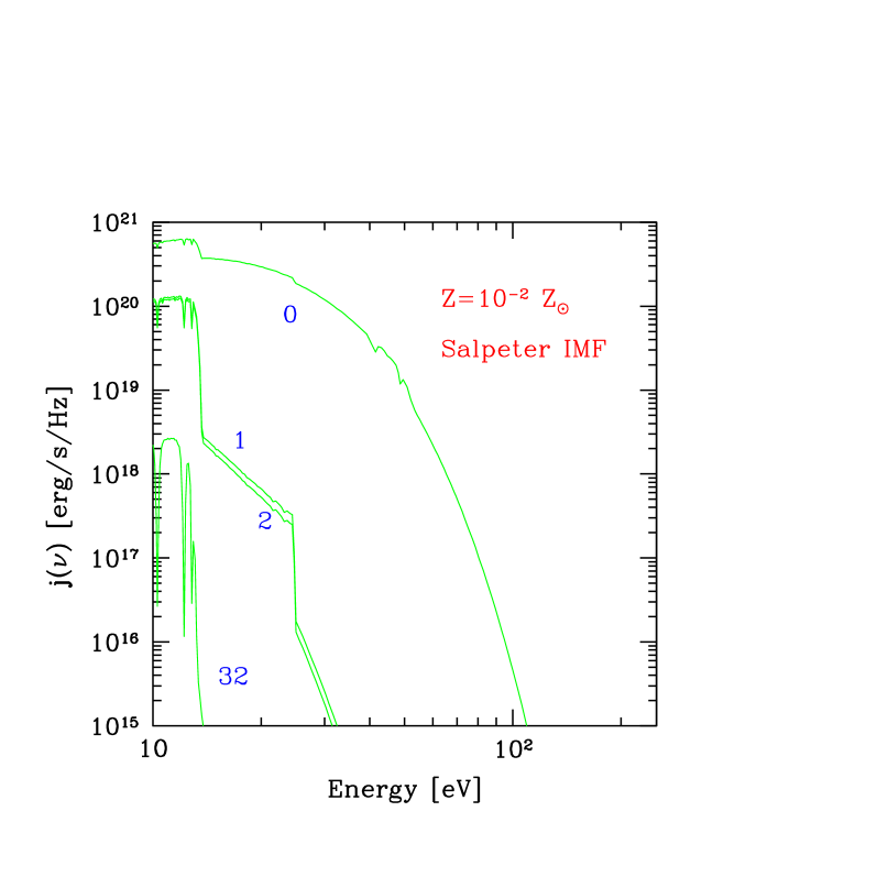
Figure 1.— Evolution of the adopted emission spectrum as a function of photon energy, at four different evolutionary times $t=(0,1,2,32)\times 10^{7}$ yr. The specific luminosity corresponds to one solar mass of stars formed.

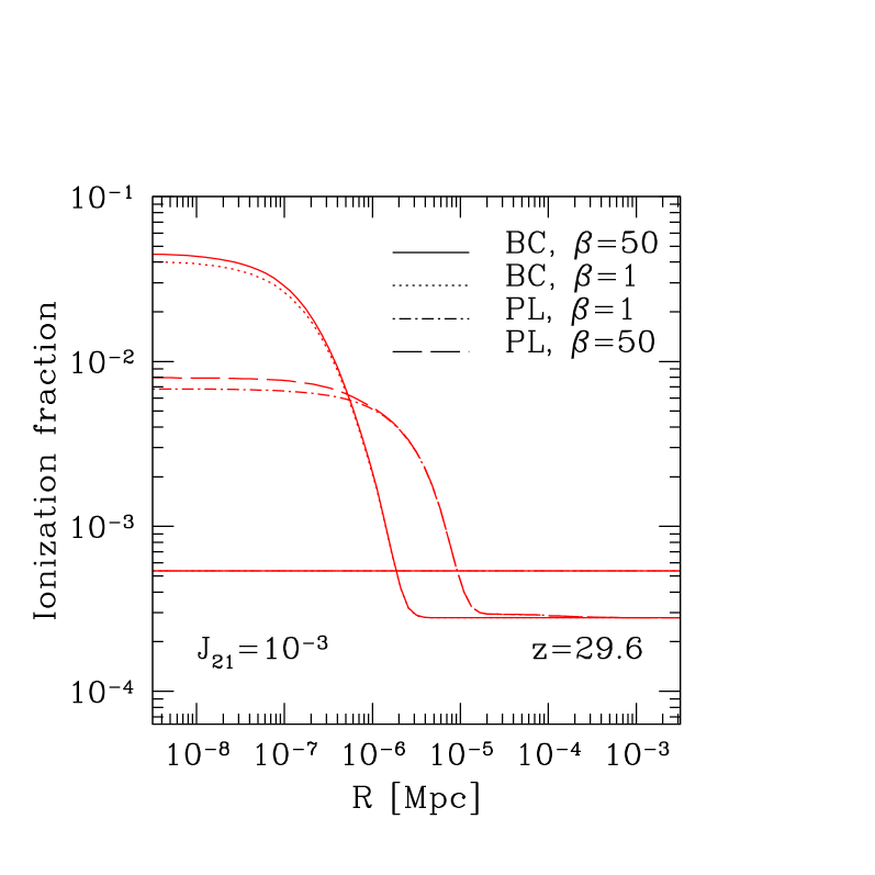
Figure 2.— Evolution of the ionized atomic hydrogen fraction as a function of depth, for a Pop III at $z=29.6$ and an incident flux $J_{s,0}=J_{21}10^{-21}$ erg s^-1 cm^-2 Hz^-1 sr^-1. The curves are derived for the BC stellar spectrum calculated at $t=2\times 10^{7}$ yr and, for comparison, for a power law spectrum (PL) with $\alpha$=1.5. Different values of the $\beta$ parameter are shown. The horizontal line represents the initial condition.

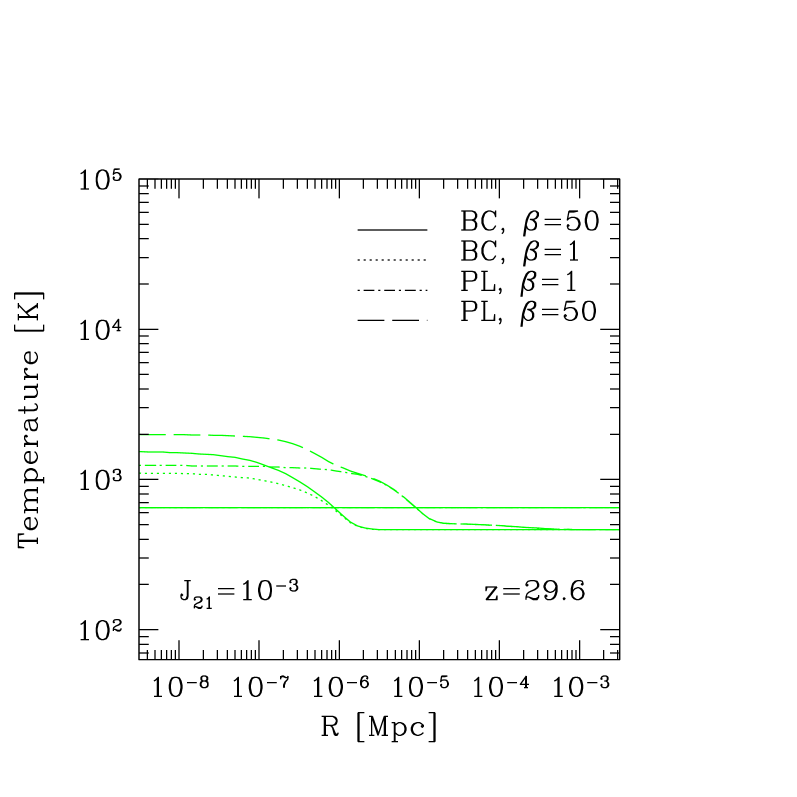
Figure 3.— As Fig. 2 for the gas temperature.

Figure 4.— As Fig. 2 for the neutral molecular hydrogen fraction.

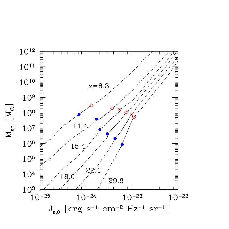
Figure 5.— Minimum total mass for self-shielding from an external incident flux with intensity $J_{s,0}$ at the Lyman limit. The curves are for different redshift: from the top to the bottom $z=$8.3, 11.4, 15.4, 18.0, 22.1, 29.6. Circles show the value of $M_{H}$ (open) and $M_{crit}$ (filled). Radiative feedback works only in the solid portions of the curves.

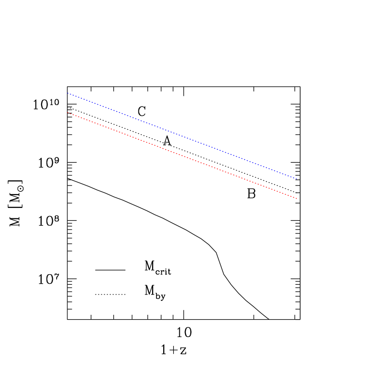
Figure 6.— Minimum total mass for collapse of an object as a function of redshift according to Tegmark et al. (1997) ($M_{crit}$, solid line) and maximum mass for blowaway as a function of redshift ($M_{by}$, dotted line). $M_{by}$ is shown for the three runs A, B, C (see Tab. 1).

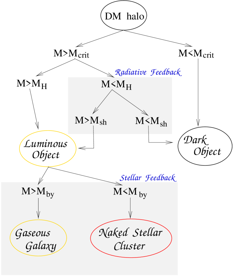
Figure 7.— Possible evolutionary tracks of objects as determined by the processes and feedbacks included in the model. Explanations are given in §6.

Figure 8.— Global spatial structure of photoionized regions at $z$=22.1 (a), 19.8 (b), 18.0 (c) and 15.4 (d).

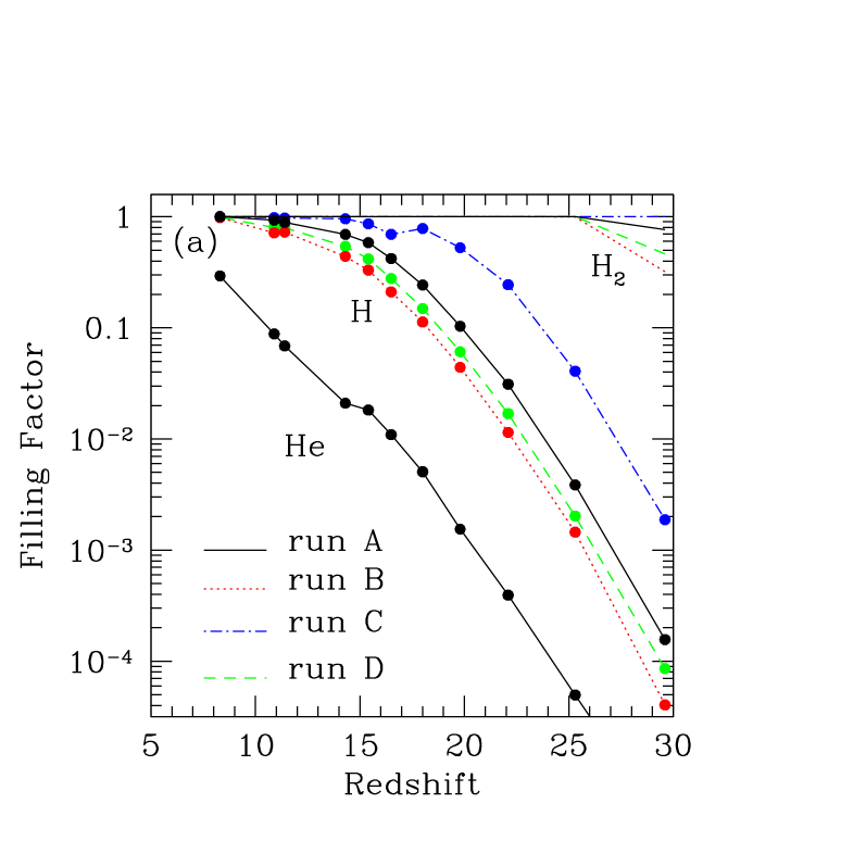
Figure 9.— (a) dissociated molecular hydrogen (upper set of lines), ionized atomic hydrogen (middle set) and doubly ionized helium (bottom line) filling factor as a function of redshift for different runs: A (solid line), B (dotted), C (dashed-dotted) and D (dashed). (b) same as (a) for runs: A (solid line), A1 (dotted) and A2 (dashed-dotted).

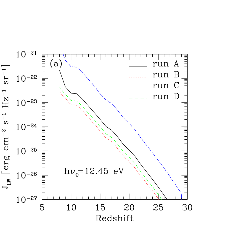
Figure 10.— (a) SUVB intensity as a function of redshift, at the central frequency of the Lyman-Werner band $h\nu_{0}$=12.45 eV for runs A-D. (b) same as (a) for runs A, A1, A2.

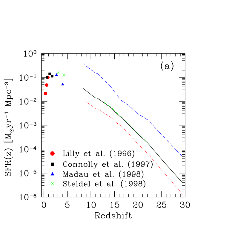
Figure 11.— (a) comoving star formation rate as a function of redshift, for runs C, D, A, B, from the top to the bottom, respectively. Data points are from Lilly et al. (1996) [circles]; Connolly et al. (1997) [squares]; Madau, Pozzetti & Dickinson (1998) [triangles] and Steidel et al. (1998) [crosses]. (b) same as (a) for runs A, A1, A2.

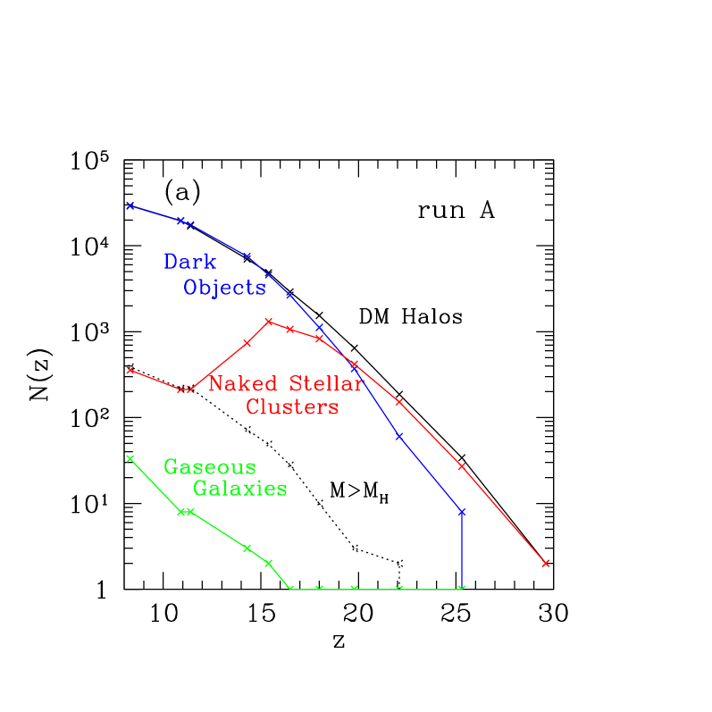
Figure 12.— (a) Number evolution of different objects in the simulation box for run A (see discussion in § 7.4) (b) same as (a) for run C.

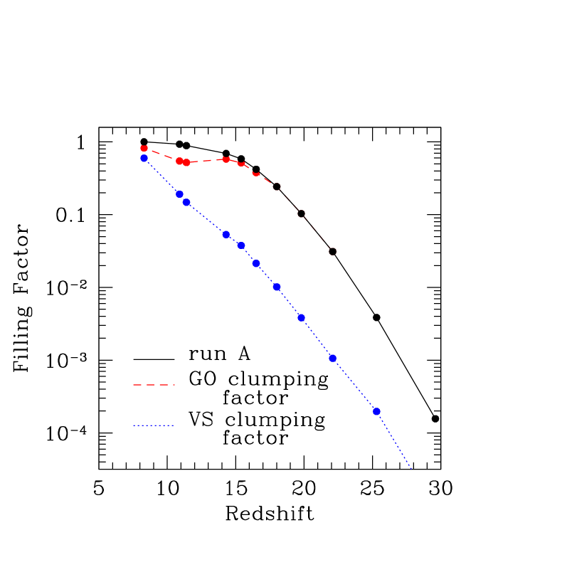
Figure 13.— Ionized atomic hydrogen filling factor as a function of redshift for different runs: A (solid line), A with the clumping factor curve of GO (dashed) and VS (dotted).

References

- (1)
- (2) Abel, T., Anninos, P., Zhang, Y. & Norman, M. L. 1997a, NewA, 2, 181.
- (3)
- (4) Abel, T., Anninos, P., Norman, M. L. & Zhang, Y. 1997b, preprint (astro-ph/9705131).
- (5)
- (6) Abel, T., Norman, M. L. & Madau, P. 1998, preprint (astro-ph/9812151).
- (7)
- (8) Abgrall, H. & Roueff, E. 1989, A&AS, 79, 313.
- (9)
- (10) Anninos, P. & Norman, M. L. 1996, ApJ, 460, 556.
- (11)
- (12) Babul, A. & Rees, M. J. 1992, MNRAS, 255, 346
- (13)
- (14) Barnes, J. & Efstathiou, G. 1987, ApJ, 319, 575.
- (15)
- (16) Baugh, C. M., Cole, S., Frenk, C. S., Lacey, C. G., 1998a, ApJ, 498, 504.
- (17)
- (18) Baugh, C. M. et al. 1998b, preprint (astro-ph/9808209).
- (19)
- (20) Benson, A. J. et al. 1999, preprint (astro-ph/9903343).
- (21)
- (22) Black, J. H. 1981, MNRAS, 197, 553.
- (23)
- (24) Bromm, V., Coppi, P. & Larson, R. 1999, in preparation
- (25)
- (26) Brown, R. L. 1971, ApJ, 164, 387.
- (27)
- (28) Blumenthal, G. R., Faber, S. M., Primack, J. R. & Rees, M. J. 1984, Nat, 311, 517.
- (29)
- (30) Bruzual, A. G. & Charlot, S. 1993, ApJ, 405, 538 (BC).
- (31)
- (32) Cen, R. 1992, ApJS, 78, 341.
- (33)
- (34) Chen, H. W., Lanzetta, K. M. & Pascarelle, S. 1999, preprint (astro-ph/9904161).
- (35)
- (36) Ciardi, B. & Ferrara, A. 1997, ApJ, 483, L5.
- (37)
- (38) Ciardi, B., Ferrara, A. & Abel, T. 1999, ApJ accepted (CFA).
- (39)
- (40) Connolly, A. L. et al. 1997, ApJ, 486, L11.
- (41)
- (42) Copi, C. J., Schramm, D. N. & Turner, M. S. 1995, Science, 267, 192.
- (43)
- (44) Cowie, L. L., Songaila, A., Kim, T. S. & Hu, E. M. 1995, AJ, 109, 1 522.
- (45)
- (46) Cowie, L. L., & Songaila, A. 1998, Nature, 344, 44.
- (47)
- (48) Davis, M., Efstathiou, G., Frenk, C. S. & White, S. D. M. 1985, ApJ, 292, 371.
- (49)
- (50) Dekel, A. & Silk, J. 1986, ApJ, 303, 39.
- (51)
- (52) Dove, J. B. & Shull, J. M. 1994, ApJ, 423, 196.
- (53)
- (54) Dove, J. B., Shull, J. M. & Ferrara, A. 1999, preprint (astro-ph/9903334).
- (55)
- (56) Eisenstein, D. J. & Hut, P. 1998, ApJ, 498, 137.
- (57)
- (58) Eke, V. R., Cole, S., Frenk, C. S., 1996, MNRAS, 282, 263.
- (59)
- (60) Federman, S. R., Glassgold, A. E. & Kwan, J. 1979, ApJ, 227, 466.
- (61)
- (62) Ferrara, A. 1998, ApJ, 499, L17.
- (63)
- (64) Ferrara, A. & Giallongo, E. 1996, MNRAS, 282, 1165.
- (65)
- (66) Ferrara, A. & Tolstoy, E. 1999, preprint (astro-ph/9905280).
- (67)
- (68) Fukugita, M. & Kawasaki, M. 1994, MNRAS, 269, 563.
- (69)
- (70) Fukugita, M., Hogan, C. J. & Peebles, P. J. E. 1998, ApJ, 503, 518.
- (71)
- (72) Galli, D. & Palla, F. 1998, A&A, 335, 403.
- (73)
- (74) Giannakopoulou-Creighton, G., Fich, M. & Wilson, C. D. 1999, preprint (astro-ph/9903334).
- (75)
- (76) Giavalisco, M. et al. 1998, ApJ, 503, 543.
- (77)
- (78) Giroux, M. L. & Shull, J. M. 1997, AJ, 113, 150.
- (79)
- (80) Giroux, M. L. & Shapiro, P. R. 1996, AJ, 102, 191.
- (81)
- (82) Gnedin, N. Y. 1998, MNRAS, 294, 407.
- (83)
- (84) Gnedin, N. Y. & Ostriker, J. P. 1997, ApJ, 486, 581 (GO).
- (85)
- (86) Governato, F. et al. 1998, Nature, 392, 359.
- (87)
- (88) Governato, F. et al. 1999, in preparation.
- (89)
- (90) Gross, M. A. K. et al. 1998, MNRAS, 301, 81.
- (91)
- (92) Gruzinov, A. & Hu, W. 1998, ApJ, 508, 435.
- (93)
- (94) Guiderdoni, G., Hivon, E., Bouchet, F. R., & Maffei, B. 1998, MNRAS, 295, 877.
- (95)
- (96) Gunn, J. E. & Peterson, B. A. 1965, ApJ, 142, 1633.
- (97)
- (98) Haiman, Z., Thoul, A. A. & Loeb, A. 1996, ApJ, 464, 523.
- (99)
- (100) Haiman, Z., Rees, M. J. & Loeb, A. 1996, ApJ, 467, 522.
- (101)
- (102) Haiman, Z., Rees, M. J. & Loeb, A. 1997, ApJ, 476, 458 (HRL).
- (103)
- (104) Haiman, Z. & Loeb, A. 1997, ApJ, 483, 21.
- (105)
- (106) Haiman, Z. & Loeb, A. 1998a, ApJ, 503, 505.
- (107)
- (108) Haiman, Z. & Loeb, A. 1998b, preprint (astro-ph/9811395).
- (109)
- (110) Haiman, Z. & Loeb, A. 1998c, preprint (astro-ph/9807070).
- (111)
- (112) Haiman, Z., Abel, T. & Rees, M. J. 1999, preprint (astro-ph/9903336).
- (113)
- (114) Hawkins, M. R. S. 1997, A&A, 328, L25.
- (115)
- (116) Hollenbach, D. & McKee, C. F. 1989, ApJ, 342, 306.
- (117)
- (118) Hughes, D. et al. 1998, Nature, 398, 241.
- (119)
- (120) Hurwitz, M., Jelinsky, P. & Dixon, W. V. 1997, ApJ, 481, L31.
- (121)
- (122) Jimenez, R., Heavens, A. F., Hawkins, M. R. S. & Padoan, P. 1997, MNRAS, 292, L5.
- (123)
- (124) Kauffmann, G. A. M., 1995, MNRAS, 274, 161.
- (125)
- (126) Klypin, A. A., Kravtsov, A. V., Valenzuela, O. & Prada, F. 1999, preprint (astro-ph/9901240).
- (127)
- (128) Knox, L, Scoccimarro, R. & Dodelson, S. 1998, Phys. Rev. Lett., 81, 2004
- (129)
- (130) Kompaneets, A. S. 1957, Soviet Phys., 4, 730.
- (131)
- (132) Lacey, C. & Cole, S. 1994, MNRAS, 271, 676.
- (133)
- (134) Lada, C. J. & Wilking, B. A. 1984, ApJ, 287, L610.
- (135)
- (136) Lada, E. A., Evans II, N. J. & Falgarone, E. 1997, ApJ, 488, 286.
- (137)
- (138) Larson, R. B. 1998, preprint (astro-ph/9808145).
- (139)
- (140) Leitherer, C., Ferguson, H. C., Heckman, T. M. & Lowental, J. D. 1995, ApJ, 454, L19.
- (141)
- (142) Lepp, S. & Shull, J. L. 1984, ApJ, 280, 465.
- (143)
- (144) Lilly, S. J., LeFevre, O., Hammer, F. & Crampton, D. 1996, ApJ, 460, L1.
- (145)
- (146) Lu, L., Sargent, W. L. W., Barlow, T. A. & Rauch, M. 1998, preprint, astro-ph/9802189.
- (147)
- (148) Mac Low, M.-M. & Ferrara, A. 1999, ApJ, 513, 142, MF.
- (149)
- (150) Madau, P., Meiksin, A. & Rees, M. 1997, ApJ, 475, 429
- (151)
- (152) Madau, P., Pozzetti, L. & Dickinson, M. E. 1998, ApJ, 498, 106.
- (153)
- (154) Madau, P., Haardt, F. & Rees, M. J. 1998, preprint (astro-ph/9809058).
- (155)
- (156) Margulis, M. & Lada, C. J. 1983, in Star Formation Workshop, ed. R. D. Wolstencroft (Edinburgh Roy. Obs.), p. 41.
- (157)
- (158) Marri, S. & Ferrara, A. 1998, ApJ, 509, 43.
- (159)
- (160) Martin, P. G., Schwarz, D. H. & Mandy, M. E. 1996, ApJ, 461, 265.
- (161)
- (162) Mathieu, R. D. 1983, ApJ 267, L97.
- (163)
- (164) Metcalfe, N. et al. 1997, Nature, 383, 326.
- (165)
- (166) Miralda-Escudé, J. 1998, ApJ, 501, 15.
- (167)
- (168) Miralda-Escudé, J., Haehnelt, M. & Rees, M. R. 1998, preprint (astr-ph/9812306).
- (169)
- (170) Mo, H. J., Mao, S. & White, S. D. M. 1998, MNRAS, 295, 319.
- (171)
- (172) Moore, B. et al. 1999a, preprint (astro-ph/9903164).
- (173)
- (174) Moore, B. et al. 1999b, submitted to ApJ.
- (175)
- (176) Nagamine, K., Cen, R. & Ostriker, J. P. 1999, preprint (astro-ph/9902327).
- (177)
- (178) Norman, M. L., Paschos, P. & Abel, T. 1998, in H2 in the Early Universe, Florence, Proc., eds. E. Corbelli, D. Galli & F. Palla, p. 455.
- (179)
- (180) Oey, Y. M. S. & Clarke, C. J. 1997, MNRAS, 289, 570.
- (181)
- (182) Oh, S. P. 1999, preprint (astro-ph/9904225).
- (183)
- (184) Omukai, K. & Nishi, R. 1999, preprint (astro-ph/9904303).
- (185)
- (186) Padmanabhan, T. 1993, Structure Formation in the Universe, (University Press: Cambridge).
- (187)
- (188) Pandey, A. K., Paliwal, D. C. & Mahra, H. S. 1990, ApJ, 362, 165.
- (189)
- (190) Pearce, F. R. & Couchman H. M. P. 1997, NewA, 2, 441.
- (191)
- (192) Peebles, P. J. E. & Dicke, R. H. 1968, ApJ, 154, 891.
- (193)
- (194) Peebles, P. J. E. 1971, Physical Cosmology, (Princeton University Press, NJ).
- (195)
- (196) Pei, Y. C., Fall, S. M. & Hauser, M. G. 1998, preprint (atro-ph/9812182).
- (197)
- (198) Planesas, P., Colina, L. & Perez-Olea, D. 1997, A&A, 325, 81.
- (199)
- (200) Press, W. H. & Schechter, P. 1974, ApJ, 187, 425 (PS).
- (201)
- (202) Razoumov, A. & Scott, D. 1998, preprint (astro-ph/9810425).
- (203)
- (204) Reimers, D. et al. 1997, A&A, 326, 489.
- (205)
- (206) Salpeter, E. E. & Hoffman, G. L. 1996, ApJ, 465, 595.
- (207)
- (208) Savaglio S. et al. 1997, A&A, 318, 347.
- (209)
- (210) Scalo, J. 1998, in The Birth of Galaxies, Blois, in press (astro-ph/9811341).
- (211)
- (212) Schmidt, M., Schneider, D. P. & Gunn, J. E. 1995, AJ, 110, 68.
- (213)
- (214) Scott, D., Rees, M. J. & Sciama, D. W. 1991, A&A, 250, 295.
- (215)
- (216) Shapiro, P. R. 1986, PASP, 98, 1014.
- (217)
- (218) Shapiro, P. R. & Giroux, M. L. 1987, ApJ, 321, L107.
- (219)
- (220) Shapiro, P. R. & Kang, H. 1987, ApJ, 318, 32.
- (221)
- (222) Shapiro, P. R. 1992, ”Chemistry in The Early Universe” in Astrochemistry of Cosmic Phenomena (IAU Symposium No. 150), ed. P. D. Singh (Kluwer Academic), pp. 73-82.
- (223)
- (224) Shapiro, P. R., Giroux, M. L. & Babul, A. 1994, ApJ, 427, 25.
- (225)
- (226) Shapiro, P. R., Raga, A. C. & Mellema, G. 1998, in H2 in the Early Universe, Florence, Proc., eds. E. Corbelli, D. Galli & F. Palla, p. 463.
- (227)
- (228) Shaver, P. A. et al. 1996, Nature, 384, 439.
- (229)
- (230) Steidel, C. C. et al. 1998, preprint (astro-ph/9811399).
- (231)
- (232) Steinmetz, M. & Bartelmann, M. 1995, MNRAS, 272, 570.
- (233)
- (234) Tegmark, M., Silk, J. & Blanchard, A. 1994, ApJ, 434, 395.
- (235)
- (236) Tegmark, M. et al. 1997, ApJ, 474, 1.
- (237)
- (238) Tegmark, M. & Peebles, P. J. E. 1998, ApJ, 500, L79.
- (239)
- (240) Thoul, A. A. & Weinberg, B. H. 1996, ApJ, 465, 608.
- (241)
- (242) Tozzi, P., Madau, P., Meiksin, A. & Rees, M. 1999, preprint (astro-ph/9905199)
- (243)
- (244) Tytler, D. et al. 1995, in QSOs Absorption Lines, Proc. ESO Workshop, ed. G. Meylan (Heidelberg: Springer), p. 289.
- (245)
- (246) Valageas, P. & Silk, J. 1999, preprint (astro-ph/9903411) (VS).
- (247)
- (248) Warren, S. J., Hewett, P. C. & Osmer, P. S. 1994, ApJ, 421, 412.
- (249)
- (250) Weil, M. L., Eke, V. R. & Efstathiou, G. 1999, preprint (astro-ph/9802311).
- (251)
- (252) White, S. D. M. & Frenk, C. S. 1991, ApJ, 379, 52
- (253)
- (254) Wilking, B. A. & Lada, C. J. 1983, ApJ, 274, 698.
- (255)