Astrometric radial velocities

Abstract

High-accuracy astrometry permits the determination of not only stellar tangential motion, but also the component along the line-of-sight. Such non-spectroscopic (i.e. astrometric) radial velocities are independent of stellar atmospheric dynamics, spectral complexity and variability, as well as of gravitational redshift. Three methods are analysed: (1) changing annual parallax, (2) changing proper motion and (3) changing angular extent of a moving group of stars. All three have significant potential in planned astrometric projects. Current accuracies are still inadequate for the first method, while the second is marginally feasible and is here applied to 16 stars. The third method reaches high accuracy ($<1$ km s^-1) already with present data, although for some clusters an accuracy limit is set by uncertainties in the cluster expansion rate.

1 Introduction

For well over a century, radial velocities for objects outside the solar system have been determined through spectroscopy, using the (Doppler) shifts of stellar spectral lines. The advent of high-accuracy (sub-milliarcsec) astrometric measurements, both on ground and in space, now permits radial velocities to be obtained by alternative methods, based on geometric principles and therefore independent of spectroscopy. The importance of such astrometric radial velocities stems from the fact that they are independent of phenomena which affect the spectroscopic method, such as line asymmetries and shifts caused by atmospheric pulsation, surface convection, stellar rotation, stellar winds, isotopic composition, pressure, and gravitational potential. Conversely, the differences between spectroscopic and astrometric radial velocities may provide information on these phenomena that cannot be obtained by other methods. Although the theoretical possibility of deducing astrometric radial velocities from geometric projection effects was noted already at the beginning of the 20th century (if not earlier), it is only recently that such methods have reached an accuracy level permitting non-trivial comparison with spectroscopic measurements.

We have analysed three methods by which astrometric radial velocities can be determined (Fig. 1). Two of them are applicable to individual, nearby stars and are based on the well understood secular changes in the stellar trigonometric parallax and proper motion. The third method uses the apparent changes in the geometry of a star cluster or association to derive its kinematic parameters, assuming that the member stars share, in the mean, a common space velocity. In Sects. 4 to 6 we describe the principle and underlying assumptions of each of the three methods and derive approximate formulae for the expected accuracy of resulting astrometric radial velocities. For the first and second methods, an inventory of nearby potential target stars is made, and the second method is applied to several of these.

However, given currently available astrometric data, only the third (moving-cluster) method is capable of yielding astrophysically interesting, sub-km s^-1 accuracy. In subsequent papers we develop in detail the theory of this method, based on the maximum-likelihood principle, as well as its practical implementation, and apply it to a number of nearby open clusters and associations, using data from the Hipparcos astrometry satellite.

2 Notations

In the following sections, $\pi$, $\mu$ and $v_{r}$ denote the trigonometric parallax of a star, its (total) proper motion, and its radial velocity. The components of $\mu$ in right ascension and declination are denoted $\mu_{\alpha*}$ and $\mu_{\delta}$, with $\mu=(\mu_{\alpha*}^{2}+\mu_{\delta}^{2})^{1/2}$. The dot signifies a time derivative, as in $\dot{\pi}\equiv{\rm d}\pi/{\rm d}t$. The statistical uncertainty (standard error) of a quantity $x$ is denoted $\epsilon(x)$. (We prefer this non-standard notation to $\epsilon_{x}$, since $x$ is itself often a subscripted variable.) $\sigma_{v}$ is used for the physical velocity dispersion in a cluster. $A=1.49598\times 10^{8}$ km is the astronomical unit; the equivalent values $4.74047$ km yr s^-1 and $9.77792\times 10^{8}$ mas km yr s^-1 are conveniently used in equations below (cf. Table 1.2.2 in Vol. 1 of ESA esa (1997)). Other notations are explained as they are introduced.

3 Astrometric accuracies

In estimating the potential accuracy of the different methods, we consider three hypothetical situations:

• Case A: a quasi-continuous series of observations over a few years, resulting in an accuracy of $\epsilon(\pi)=1$ mas (milliarcsec) for the trigonometric parallaxes and $\epsilon(\mu)=1$ mas yr^-1 for the proper motions.

• Case B: similar to Case A, only a thousand times better, i.e. $\epsilon(\pi)=1$ $\mu$as (microarcsec) and $\epsilon(\mu)=1$ $\mu$as yr^-1.

• Case C: two sets of measurements, separated by an interval of 50 yr, where each set has the same accuracy as in Case B. The much longer-time baseline obviously allows a much improved determination of the accumulated changes in parallax and proper motion.

The accuracies assumed in Case A are close to what the Hipparcos space astrometry mission (ESA esa (1997)) achieved for its main observation programme of more than 100 000 stars. Current ground-based proper motions may be slightly better than this, but not by a large factor. This case therefore represents, more or less, the state-of-the-art accuracy in optical astrometry. Accuracies in the 1 to 10 $\mu$as range are envisaged for some planned or projected space astrometry missions, such as GAIA (Lindegren & Perryman lindegren96 (1996)) and SIM (Unwin et al. unwin (1998)). The duration of such a mission is here assumed to be about 5 years. Using the longer-time baselines available with ground-based techniques, similar performance may in the future be reached with the most accurate ground-based techniques (Pravdo & Shaklan pravdo (1996); Shao shao (1996)). Case B therefore corresponds to what we could realistically hope for within one or two decades. Case C, finally, probably represents an upper limit to what is practically feasible in terms of long-term proper-motion accuracy, not to mention the patience of astronomers.

Figure 1: Three methods to astrometrically determine stellar radial motion: a Changing trigonometric parallax $\pi$; b Perspective change in the proper motion $\mu$; c Changing angular separation $\rho$ of stars sharing the same space velocity, e.g. in a moving cluster.

4 Radial velocity from changing annual parallax

The most direct and model-independent way to determine radial velocity by astrometry is to measure the secular change in the trigonometric parallax (Fig. 1a). The distance $b$ (from the solar system barycentre) is related to parallax $\pi$ through $b=A/\sin\pi\simeq A/\pi$. Since $v_{r}=\dot{b}$, the radial velocity is

$$v_{r}=-A\,\frac{\dot{\pi}}{\pi^{2}}\,,$$ (1)

where $A$ is the astronomical unit (Sect. 2). The equivalent of Eq. (1) was derived by Schlesinger (schlesinger (1917)), who concluded that the parallax change is very small for every known star. However, although extremely accurate parallax measurements are obviously required, the method is not as unrealistic as it may seem at first. To take a specific, if extreme, example: for Barnard’s star (Gl 699 = HIP 87937), with $\pi=549$ mas and $v_{r}=-110$ km s^-1, the expected parallax rate is $\dot{\pi}=+34\leavevmode\nobreak\ \mu$as yr^-1. According to our discussion in Sect. 3 this will almost certainly be measurable in the near future.

It can be noted that the changing-parallax method, in contrast to the methods described in Sect. 5 and 6, does not depend on the object having a large and uniform space motion, and would therefore be applicable to all stars within a few parsecs of the Sun.

Table 1: Number of target stars, and achievable accuracy in the radial velocity, as obtained from the changing annual parallax. $n$ = number of stars with parallax greater than $\pi$ in the Third Catalogue of Nearby Stars (Gliese & Jahreiß gliese (1991)); $\epsilon(v_{r})$ = predicted accuracy according to Eqs. (2) and (3). Case B: space astrometry mission lasting $L=5$ yr and yielding parallaxes with standard error $\epsilon(\pi)=1\leavevmode\nobreak\ \mu$as and consequently $\epsilon(\dot{\pi})=0.69\leavevmode\nobreak\ \mu$as yr^-1; Case C: combination of two such measurements, $\epsilon(\pi_{1})=\epsilon(\pi_{2})=1\leavevmode\nobreak\ \mu$as, with a large epoch difference, $T=50$ yr.

$\pi$	$n$	$\epsilon(v_{r})$ [km s-1]
[mas]		Case B	Case C
740	3	01.2	0.05
300	14	07.5	0.30
200	60	17.0	0.70
100	326	68.0	2.80

4.1 Achievable accuracy

The accuracy in $v_{r}$ is readily estimated from Eq. (1) for a given accuracy in $\dot{\pi}$, since the contribution of the parallax uncertainty to the factor $A/\pi^{2}$ is negligible. The achievable accuracy in $\dot{\pi}$ depends both on the individual astrometric measurements and on their number and distribution in time. Concerning the temporal distribution of the measurements we consider two limiting situations:

Quasi-continuous observation. The measurements are more or less uniformly spread out over a time period of length $L$ centred on the epoch $t_{0}$. This is a good approximation to the way a single space mission would typically be operated; for example, Hipparcos had $L\simeq 3$ yr and $t_{0}\simeq 1991.25$. In such a case there exist simple (mean) relations between how accurately the different astrometric parameters of the same star can be derived, depending on $L$. For instance, $\epsilon(\mu_{\delta})\simeq(\sqrt{12}/L)\epsilon(\delta)$, if $\epsilon(\mu_{\delta})$ is the accuracy of the proper motion in declination and $\epsilon(\delta)$ that of the declination at $t_{0}$. This approximation is applicable to Case A and B as defined in Sect. 3.

Two-epoch observation. Two isolated parallax or proper-motion measurements are taken, separated by a long time interval (say, $T$ years) during which no observation takes place. Each measurement must actually be the result of a series covering at least a year or so, but the duration of each such series is assumed to be negligible compared with $T$. This could be two similar space missions separated by several decades and is applicable to Case C in Sect. 3.

For quasi-continuous observation we may assume that the parallax variation is linear over the observation period $L$. Thus, $\pi(t)=\pi_{0}+(t-t_{0})\dot{\pi}$, where $\pi_{0}$ and $\dot{\pi}$ are two parameters to be determined from the observations. There exists an approximate relation between the accuracies of these two parameters that is similar to that between the proper motion and the position at the mean epoch, viz. $\epsilon(\dot{\pi})=(\sqrt{12}/L)\epsilon(\pi_{0})$. Moreover, the estimates of the two parameters are uncorrelated, so $\epsilon(\pi_{0})$ equals the accuracy $\epsilon(\pi)$ of a parallax determination in the absence of the parallax-change term; thus

$$\epsilon(v_{r})\simeq\sqrt{12}\,A\,\frac{\epsilon(\pi)}{L\pi^{2}}\,.$$ (2)

In the case of a two-epoch observation, let us assume that independent parallax measurements $\pi_{1}$ and $\pi_{2}$ are made at epochs $t_{1}$ and $t_{2}=t_{1}+T$. The estimated rate of change is $\dot{\pi}=(\pi_{2}-\pi_{1})/T$. With $\epsilon(\pi_{1})$ and $\epsilon(\pi_{2})$ denoting the accuracies of the two measurements, we have $\epsilon(\dot{\pi})=[\epsilon(\pi_{1})^{2}+\epsilon(\pi_{2})^{2}]^{1/2}/T$ and consequently

$$\epsilon(v_{r})\simeq\frac{A}{T\pi^{2}}\,\left[\epsilon(\pi_{1})^{2}+\epsilon(\pi_{2})^{2}\right]^{1/2}\,.$$ (3)

For given observational errors we find, from both Eq. (2) and (3), that the radial-velocity error is simply a function of distance. The number of potential target stars for a certain maximum radial-velocity uncertainty is therefore given by the total number of stars within the corresponding maximum distance. Table 1 gives the actual numbers of such stars, and the observational accuracies that may be reached.

5 Radial velocity from changing proper motion (perspective acceleration)

To a good approximation, single stars move with uniform linear velocity through space. For a given linear tangential velocity, the angular velocity (or proper motion $\mu$), as seen from the Sun, varies inversely with the distance to the object. However, the tangential velocity changes due to the varying angle between the line of sight and the space-velocity vector (Fig. 1b). As is well known (e.g. van de Kamp vdkamp67 (1967), Murray murray (1983)) the two effects combine to produce an apparent (perspective) acceleration of the motion on the sky, or a rate of change in proper motion amounting to $\dot{\mu}=-2\mu v_{r}/b$. With $b=A/\pi$ we find

$$v_{r}=-A\,\frac{\dot{\mu}}{2\pi\mu}\,.$$ (4)

Schlesinger (schlesinger (1917)) derived the equivalent of this equation, calculated the perspective acceleration for Kapteyn’s and Barnard’s stars (cf. Table 2) and noted that, if accurate positions are acquired over long periods of time, “we shall be in position to determine the radial velocities of these stars independently of the spectroscope and with an excellent degree of precision”. The equation for the perspective acceleration was earlier derived by Seeliger (seeliger (1901)) and used by Ristenpart (ristenpart (1902)) in an (unsuccessful) attempt to determine $\dot{\mu}$ observationally for Groombridge 1830. A major consideration for Ristenpart seems to have been the possibility to derive the parallax from the apparent acceleration in combination with a spectroscopic radial velocity. Such a determination of ‘acceleration parallaxes’ was also considered by Eichhorn (eichhorn81 (1981)).

Table 2: Nearby high-proper-motion stars suitable for the determination of radial velocity from changing proper motion (perspective acceleration). All known objects with a parallax-proper-motion product greater than 0.5 arcsec² yr^-1 are included. Data are from the Hipparcos Catalogue (ESA esa (1997)) where available, otherwise from the preliminary version of the Third Catalogue of Nearby Stars, CNS3 (Gliese & Jahreiß gliese (1991)). Columns: CNS3 = identifier in CNS3; HD = identifier in the HD/HDE catalogue; HIP = identifier in the Hipparcos Catalogue; Sp = spectral classification in CNS3; $V$ = visual magnitude; $b$ = distance from the Sun; $\pi\mu$ = product of parallax and proper motion; $\epsilon(v_{r})$ = predicted accuracy of the astrometric radial velocity (Case B: space astrometry mission lasting $L=5$ yr and yielding an accuracy of $\epsilon(\mu)=1\leavevmode\nobreak\ \mu$as yr^-1 for the mean proper motion and consequently $\epsilon(\dot{\mu})=1.55\leavevmode\nobreak\ \mu$as yr^-2 for the acceleration; Case C: the combination of two such measurements with $\epsilon(\mu_{1})=\epsilon(\mu_{2})=1\leavevmode\nobreak\ \mu$as yr^-1 having an epoch difference $T=50$ yr). In the last column, $P$ is the orbital period of a binary. Possibly, the star CF UMa does not exist, being an erroneous catalogue entry.

CNS3	HD	HIP	Sp	$V$	$b$	$\pi\mu$	$\epsilon(v_{r})$ [km s-1]		Remark
					[pc]	[arcsec2 yr-1]	Case B	Case C
Gl 699		87937	sdM4	9.5	1.8	5.69	0.13	0.01	Barnard’s star
Gl 551		70890	M5Ve	11.0	1.3	2.98	0.25	0.01	$\alpha$ Cen C (Proxima)
Gl 559B	128621	71681	K0V	1.4	1.3	2.76	0.27	0.01	$\alpha$ Cen B
Gl 559A	128620	71683	G2V	0.0	1.3	2.75	0.28	0.01	$\alpha$ Cen A (AB: $P=80$ yr)
Gl 191	33793	24186	M0V	8.9	3.9	2.21	0.34	0.01	Kapteyn’s star
Gl 887	217987	114046	M2Ve	7.4	3.3	2.10	0.36	0.01
Gl 406			M6	13.5	2.4	1.96	0.38	0.01	Wolf 359
Gl 411	95735	54035	M2Ve	7.5	2.5	1.88	0.40	0.01
Gl 820A	201091	104214	K5Ve	5.2	3.5	1.52	0.50	0.02	61 Cyg A
Gl 820B	201092	104217	K7Ve	6.1	3.5	1.48	0.51	0.02	61 Cyg B (AB: $P=700$ yr)
Gl 1	225213	439	M4V	8.6	4.4	1.40	0.54	0.02
Gl 845	209100	108870	K5Ve	4.7	3.6	1.30	0.58	0.02	$\epsilon$ Ind
Gl 65A			dM5.5e	12.6	2.6	1.28	0.59	0.02
Gl 65B			dM5.5e	12.7	2.6	1.28	0.59	0.02	UV Cet (AB: $P=27$ yr)
Gl 273		36208	M3.5	9.8	3.8	0.98	0.77	0.03	Luyten’s star
Gl 866AB			M5e	12.3	3.4	0.96	0.79	0.03	$P=2.2$ yr
Gl 412A		54211	M2Ve	8.8	4.8	0.93	0.81	0.03
Gl 412B			M6e	14.4	5.3	0.86	0.88	0.03	WX UMa
Gl 825	202560	105090	M0Ve	6.7	3.9	0.88	0.86	0.03
Gl 15A	1326	1475	M2V	8.1	3.6	0.82	0.92	0.03	GX And
Gl 15B			M6Ve	11.1	3.6	0.84	0.90	0.03	GQ And (AB: $P=2600$ yr)
Gl 166A	26965	19849	K1Ve	4.4	5.0	0.81	0.94	0.03	40 Eri A ($o^{2}$ Eri)
Gl 166B	26976		DA4	9.5	4.8	0.84	0.90	0.03	40 Eri B (BC: $P=250$ yr)
Gl 166C			dM4.5e	9.5	4.8	0.84	0.90	0.03	DY Eri
Gl 299			dM5	12.8	6.8	0.77	0.98	0.04	Ross 619
Gl 451A	103095	57939	G8VI	6.4	9.2	0.77	0.98	0.04	Groombridge 1830
Gl 451B			—	12	9.2	0.82	0.92	0.03	CF UMa (non-existent star?)
Gl 35		3829	DZ7	12.4	4.4	0.68	1.10	0.04	van Maanen 2
Gl 725B	173740	91772	dM5	9.7	3.6	0.66	1.20	0.04	AB: $P=400$ yr
Gl 725A	173739	91768	dM4	8.9	3.6	0.63	1.20	0.04
Gl 440		57367	DQ6	11.5	4.6	0.58	1.30	0.05
Gl 71	10700	8102	G8Vp	3.5	3.6	0.53	1.40	0.05	$\tau$ Cet
Gl 754			M4.5	12.2	5.7	0.52	1.50	0.05
Gl 139	20794	15510	G5V	4.3	6.1	0.52	1.50	0.05	82 Eri
Gl 905			dM6	12.3	3.2	0.51	1.50	0.05
Gl 244A	48915	32349	A1V	$-1.4$	2.6	0.51	1.50	0.05	$\alpha$ CMa (Sirius)
Gl 244B			DA2		2.6	0.51	1.50	0.05	AB: $P=50$ yr
Gl 53A	6582	5336	G5VI	5.2	7.6	0.50	1.50	0.06	$\mu$ Cas
Gl 53B			—	11	7.6	0.51	1.50	0.06	AB: $P=20$ yr

Subsequent attempts to determine the perspective acceleration of Barnard’s star by Lundmark & Luyten (lundmark (1922)), Alden (alden (1924)) and van de Kamp (1935b ) yielded results that were only barely significant or (in retrospect) spurious. Meanwhile, Russell & Atkinson (russell (1931)) suggested that the white dwarf van Maanen 2 might exhibit a gravitational redshift of several hundred km s^-1 and that this could be distinguished from a real radial velocity through measurement of the perspective acceleration. The astrophysical relevance of astrometric radial-velocity determinations was thus already established (Oort oort (1932)).

In relatively recent times, the perspective acceleration was successfully determined for Barnard’s star by van de Kamp (vdkamp62 (1962), vdkamp63 (1963), vdkamp67 (1967), vdkamp70 (1970), vdkamp81 (1981)); for van Maanen 2 by van de Kamp (vdkamp71 (1971)), Gatewood & Russell (gatewood (1974)) and Hershey (hershey (1978)); and for Groombridge 1830 by Beardsley et al. (beardsley (1974)). Among these determinations the highest precisions, in terms of the astrometric radial velocity, were obtained for Barnard’s star (corresponding to $\pm 4$ km s^-1; van de Kamp vdkamp81 (1981)) and van Maanen 2 ($\pm 15$ km s^-1; Gatewood & Russell gatewood (1974)).

Our application of the method, combining Hipparcos measurements with data in the Astrographic Catalogue, yielded radial velocities for 16 objects, as listed in Table 3.

5.1 Achievable accuracy

The accuracy of the radial velocity calculated from Eq. (4) can be estimated as in Sect. 4.1. It depends on the parallax-proper-motion product $\pi\mu$. The most promising targets for this method are listed in Table 2, which contains the known nearby stars ranked after decreasing $\pi\mu$.

For quasi-continuous observation during a period of length $L$ we may use a quadratic model for the angular position $\phi$ of the star along the great-circle arc: $\phi(t)=\phi(t_{0})+(t-t_{0})\mu_{0}+{\scriptstyle\frac{1}{2}}(t-t_{0})^{2}\dot{\mu}$. Here $\mu_{0}$ is the proper motion at the central epoch $t_{0}$. The estimates of $\mu_{0}$ and $\dot{\mu}$ are found to be uncorrelated and their errors related by $\epsilon(\dot{\mu})=(\sqrt{60}/L)\epsilon(\mu_{0})$. Consequently,

$$\epsilon(v_{r})\simeq\sqrt{15}\,A\,\frac{\epsilon(\mu)}{L\pi\mu}$$ (5)

where $\epsilon(\mu)$ is the accuracy of proper-motion measurements in the absence of temporal changes. We neglect the (small) contribution to $\epsilon(v_{r})$ from the uncertainty in the denominator $\pi\mu$.

For a two-epoch observation, consider proper-motion measurements $\mu_{1}$ and $\mu_{2}$ made around $t_{1}$ and $t_{2}=t_{1}+T$. The estimated acceleration is $\dot{\mu}=(\mu_{2}-\mu_{1})/T$. Provided the two observation intervals centred on $t_{1}$ and $t_{2}$ do not overlap, the measurements are independent, yielding the standard error $\epsilon(\dot{\mu})=[\epsilon(\mu_{1})^{2}+\epsilon(\mu_{2})^{2}]^{1/2}/T$. For the radial velocity this gives

$$\epsilon(v_{r})\simeq\frac{A}{T\pi\mu}\,\left[\epsilon(\mu_{1})^{2}+\epsilon(\mu_{2})^{2}\right]^{1/2}\,.$$ (6)

Based on these formulae, Table 2 gives the potential radial-velocity accuracy for the two cases B and C defined in Sect. 3.

In a two-epoch observation we normally have, in addition, a very good estimate of the mean proper motion between $t_{1}$ and $t_{2}$, provided the positions $\phi_{1}$ and $\phi_{2}$ at these epochs are accurately known. In the previous quadratic model we may take the reference epoch to be $t_{0}=(t_{1}+t_{2})/2$ and find $\mu_{0}=(\phi_{2}-\phi_{1})/T$ with standard error $\epsilon(\mu_{0})=[\epsilon(\phi_{1})^{2}+\epsilon(\phi_{2})^{2}]^{1/2}/T$. The three proper-motion estimates $\mu_{0}$, $\mu_{1}$ and $\mu_{2}$ (referred to $t_{0}$, $t_{1}$ and $t_{2}$) are mutually independent and may be combined in a least-squares estimate of $\dot{\mu}$. If $\epsilon(\mu_{1})=\epsilon(\mu_{2})$ (equal weight at $t_{1}$ and $t_{2}$), then it is found that $\mu_{0}$ does not contribute at all to the determination of $\dot{\mu}$, and the standard error is still given by Eq. (6). If, on the other hand, the two observation epochs are not equivalent, then some improvement can be expected by introducing the position measurements.

An important special case is when there is just a position (no proper motion) determined at one of the epochs, say $t_{1}$. This is however equivalent to the two independent proper-motion determinations $\mu_{0}$ at $t_{0}=(t_{1}+t_{2})/2$, and $\mu_{2}$ at $t_{2}$, separated by $t_{2}-t_{0}=T/2$. Applying Eq. (6) on this case yields

$$\epsilon(v_{r})\simeq\frac{2A}{T\pi\mu}\,\left[\frac{\epsilon(\phi_{1})^{2}+\epsilon(\phi_{2})^{2}}{T^{2}}+\epsilon(\mu_{2})^{2}\right]^{1/2}\,.$$ (7)

This formula is applicable on the combination of a recent position and proper-motion measurement (e.g. by Hipparcos) with a position derived from old photographic plates (e.g. the Astrographic Catalogue). Taking $t_{1}\sim 1907$, $\epsilon(\phi_{1})\simeq 200$ mas as representative for the Astrographic Catalogue, and $t_{2}=1991.25$, $\epsilon(\phi_{2})\simeq 1$ mas, $\epsilon(\mu_{2})\simeq 1$ mas yr^-1 for Hipparcos, we find $\epsilon(v_{r})\simeq(60\leavevmode\nobreak\ \mbox{km\leavevmode\nobreak\ s${}^{-1}$\leavevmode\nobreak\ arcsec${}^{2}$\leavevmode\nobreak\ yr${}^{-1}$})/(\pi\mu)$. With such data, moderate accuracies of a few tens of km s^-1 can be reached for several stars (Sect. 5.3).

5.2 Effects of gravitational perturbations

The perspective-acceleration method depends critically on the assumption that the star moves with uniform space motion relative the observer. The presence of a real acceleration of their relative motions, caused by gravitational action of other bodies, would bias the calculated astrometric radial velocity by $-g_{t}/2\mu$, where $g_{t}$ is the tangential component of the relative acceleration. The acceleration towards the Galactic centre caused by the smoothed Galactic potential in the vicinity of the Sun is $g\simeq 2\times 10^{-13}$ km s^-2. For a hypothetical observer near the Sun but unaffected by this acceleration, the maximum bias would be 0.06 km s^-1 for Barnard’s star, and 0.17 km s^-2 for Proxima. However, since real observations are made relative the solar-system barycentre, which itself is accelerated in the Galactic gravitational field, the observed (differential) effect will be very much smaller.

In the case of Proxima the acceleration towards $\alpha$ Cen AB is of a similar magnitude as the Galactic acceleration. For the several orbital binaries in Table 2 the curvature of the orbit is much greater than the perspective acceleration. Application of this method will therefore require careful correction for all known perturbations: the possible presence of long-period companions may introduce a considerable uncertainty.

Among other effects which may have to be considered are light-time effects which, to first order in $c^{-1}$, may require a correction of $-v_{t}^{2}/2c$ on the right-hand side of Eq. (4), where $v_{t}$ is the tangential velocity. For typical high-velocity (Population II) stars the correction is 0.1–0.2 km s^-1. At this accuracy level, the precise definition of the radial-velocity concept itself requires careful consideration (Lindegren et al. lindegren99 (1999)).

Table 3: Astrometric radial velocities, obtained by combining positions and proper motions from Hipparcos (epoch 1991.25) with old position measurements from the Astrographic Catalogue. Spectroscopic radial velocities are also given (from Turon et al. turon (1998)). Data for the binary 61 Cyg = HIP 104214+104217 = AC 1382645+1382649 refer to its mass centre, assuming a mass ratio of 0.90. Two solutions are given: the first based on Hipparcos and AC data alone; the second (marked *) includes Bessel’s visual measurements from 1838.

HIP	AC 2000		Radial velocity, $v_{r}$ [km s-1]		Remark
	No.	Epoch	Astrom.	Spectr.
000439	3152964	1912.956	00$+7.0\leavevmode\nobreak\ \pm\phantom{0}29.7$	0$+22.9$
001475	1406215	1898.435	0$-40.8\leavevmode\nobreak\ \pm\phantom{0}36.1$	0$+12.0$	GX And
005336	1721511	1913.868	$-106.4\leavevmode\nobreak\ \pm\phantom{0}82.7$	0$-98.0$	$\mu$ Cas
15510	3488626	1901.018	0$+89.6\leavevmode\nobreak\ \pm\phantom{0}59.1$	0$+86.8$	82 Eri
19849	2125614	1892.970	0$-73.2\leavevmode\nobreak\ \pm\phantom{0}32.8$	0$-42.6$	40 Eri
24186	3505363	1899.058	$+249.4\leavevmode\nobreak\ \pm\phantom{0}13.7$	$+245.5$	Kapteyn’s star
36208	282902	1908.859	0$-33.7\leavevmode\nobreak\ \pm\phantom{0}38.4$	0$+18.7$	Luyten’s star
54035	1340883	1930.895	0$+22.0\leavevmode\nobreak\ \pm\phantom{0}36.1$	0$-85.6$
54211	1463341	1895.620	0$+58.6\leavevmode\nobreak\ \pm\phantom{0}30.5$	0$+67.5$
57367	4195112	1924.492	0$+43.1\leavevmode\nobreak\ \pm\phantom{}106.4$	—
57939	1342199	1930.260	$-139.5\leavevmode\nobreak\ \pm\phantom{0}86.1$	0$-98.0$	Groombridge 1830
87937	146626	1905.979	$-101.9\leavevmode\nobreak\ \pm\phantom{00}6.5$	$-109.7$	Barnard’s star
104214/217	1382645/649	1921.699	0$-12.2\leavevmode\nobreak\ \pm\phantom{0}34.5$	0$-64.5$	61 Cyg
104214/217	1382645/649	1921.699	0$-68.0\leavevmode\nobreak\ \pm\phantom{0}11.1$ *	”	”
105090	3462277	1905.316	0$-25.0\leavevmode\nobreak\ \pm\phantom{0}40.9$	0$+23.6$
108870	4384302	1901.189	0$-64.1\leavevmode\nobreak\ \pm\phantom{0}23.6$	0$-40.0$	$\epsilon$ Ind
114046	3355101	1913.368	0$+54.0\leavevmode\nobreak\ \pm\phantom{0}19.7$	00$+9.5$

5.3 Results from observed proper-motion changes

Past determinations of the perspective acceleration, e.g. by van de Kamp (vdkamp81 (1981)) and Gatewood & Russell (gatewood (1974)), were based on photographic observations collected over several decades, in which the motion of the target star was measured relative to several background (reference) stars. One difficulty with the method has been that the positions and motions of the reference stars are themselves not accurately known, and that small errors in the reference data could cause a spurious acceleration of the target star (van de Kamp 1935a ).

The Hipparcos Catalogue (ESA esa (1997)) established a very accurate and homogeneous positional reference frame over the whole sky. Using the proper motions, this reference frame can be extrapolated backwards in time. It is then possible to re-reduce measurements of old photographic plates, and express even century-old stellar positions in the same reference frame as modern observations. This should greatly facilitate the determination of effects such as the perspective acceleration, which are sensitive to systematic errors in the reference frame.

As part of the Carte du Ciel project begun more than a century ago, an astrographic programme to measure the positions of all stars down to the 11th magnitude was carried out and published as the Astrographic Catalogue, AC (see Eichhorn eichhorn74 (1974) for a description). After transfer to electronic media, the position measurements have been reduced to the Hipparcos reference frame (Nesterov et al. nesterov (1998), Urban et al. urban (1998)). The result is a positional catalogue of more than 4 million stars with a mean epoch around 1907 and a typical accuracy of about 200 mas. We have used the version known as AC 2000 (Urban et al. urban (1998)), available on CD-ROM from the US Naval Observatory, to examine the old positions of all the stars with HIP identifiers in Table 2.

For the stars in Table 3 we successfully matched the AC positions with the positions extrapolated backwards from the Hipparcos Catalogue and hence could calculate the astrometric radial velocities. Other potential targets in Table 2 were either outside the magnitude range of AC 2000 (e.g. $\alpha$ Cen and Proxima) or lacked an accurate proper motion from Hipparcos (e.g. van Maanen 2 and HIP 91768+91772).

The basic procedure was as follows. The rigorous epoch transformation algorithm described in Sect. 1.5.5 of the Hipparcos Catalogue, Vol. 1, was used to propagate the Hipparcos position and its covariance matrix to the AC 2000 epoch relevant for each star. This extrapolated position was compared with the actual measured position in AC 2000, assuming a standard error of 200 mas in each coordinate for the latter. A $\chi^{2}$ goodness-of-fit was then calculated from the position difference and the combined covariance of the extrapolated and measured positions. The epoch transformation algorithm requires that the radial velocity is known. The radial velocity was therefore varied until the $\chi^{2}$ attained its minimum value. The $\pm$1$\sigma$ confidence interval given in the table was obtained by modifying the radial velocity until the $\chi^{2}$ had increased by one unit above the minimum.

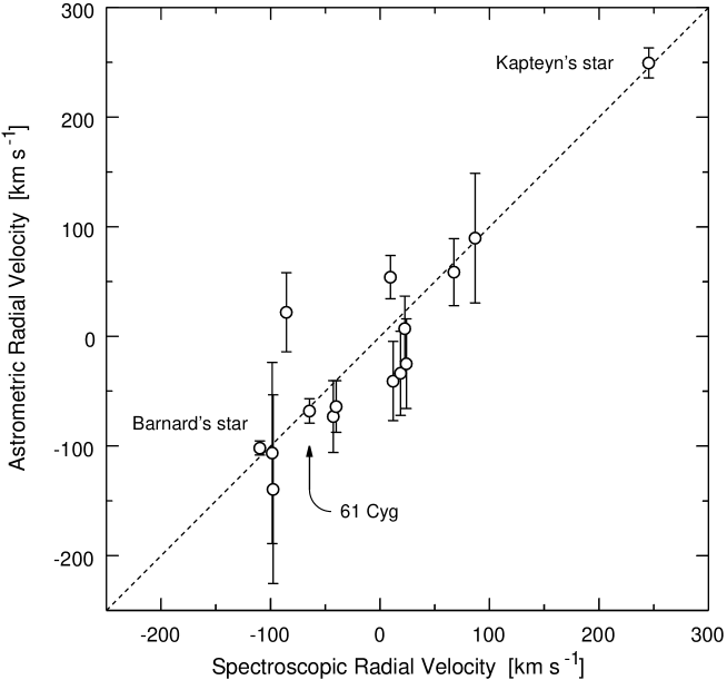
Figure 2: Comparison of the astrometric radial velocities in Table 3 with their spectroscopic counterparts. The straight line is the expected relationship $v_{r}(\mbox{astrom.})\simeq v_{r}(\mbox{spectr.})$. The three most accurate determinations are indicated.

For some of the stars, data had to be corrected for duplicity or known orbital motion. The solutions for the resolved binary 61 Cyg (HIP 104214+104217) refer to the mass centre, assuming a mass ratio of $M_{\rm B}/M_{\rm A}=0.90$, as estimated by means of standard isochrones from the absolute magnitudes and colour indices of the components (Söderhjelm, private communication). For the astrometric binary $\mu$ Cas (HIP 5336) the Hipparcos data explicitly refer to the mass centre using the orbit by Heintz & Cantor (heintz (1994)); the same orbit was used to correct the AC position of the primary to the mass centre. No correction for orbital motion was used for GX And and 40 Eri.

Table 3 gives two solutions for 61 Cyg. The first solution was obtained as described above, using only the Hipparcos data plus the AC positions for the two components. The second solution, marked with an asterisk in the table, was derived by including also the observations by Bessel (bessel39 (1839)) from his pioneering determination of the star’s parallax. Bessel measured the angular distances from the geometrical centre (half-way between the components) of 61 Cyg to two reference stars, called $a$ and $b$ in his paper. After elimination of aberration, proper motion and parallax, he found the distances $461.6171\pm 0.015$ arcsec and $706.2791\pm 0.017$ arcsec for the beginning of year 1838 (B1838.0 = J1838.0022). The uncertainties are our estimates (standard errors) based on the scatter of the residuals in Bessel’s solution ‘II’. We identified the reference stars in AC 2000 and in the Tycho Catalogue (ESA esa (1997)) as $a$ = AC 1382543 = TYC 3168 708 1 and $b$ = AC 1382712 = TYC 3168 1106 1. Extrapolating the positions from these catalogues back to B1838 allowed us to compute the position of the geometrical centre of 61 Cyg in the Hipparcos/Tycho reference frame. This could then be transformed to the position of the mass centre, using Bessel’s own measurement of the separation and position angle in 61 Cyg and the previously assumed mass ratio. Actually, all the available data were combined into a $\chi^{2}$ goodness-of-fit measure and the radial velocity was varied in order to find the minimum and the $\pm$1$\sigma$ confidence interval. This gave $v_{r}=-68.0\pm 11.1$ km s^-1.

Table 3 also gives the spectroscopic radial velocities when available in the literature. A comparison between the astrometric and spectroscopic radial velocities is made in Fig. 2. Given the stated confidence intervals, the agreement is in all cases rather satisfactory. The exercise demonstrates the basic feasibility of this method, but also hints at some of the difficulties in applying it to non-single stars.

6 Radial velocity from changing angular extent (moving-cluster method)

The moving-cluster method is based on the assumption that the stars in a cluster move through space essentially with a common velocity vector. The radial-velocity component makes the cluster appear to contract or expand due to its changing distance (Fig. 1c). The relative rate of apparent contraction equals the relative rate of change in distance to the cluster. This can be converted to a linear velocity (in km s^-1) if the distance to the cluster is known, e.g. from trigonometric parallaxes. In practice, the method amounts to determining the space velocity of the cluster, i.e. the convergent point and the speed of motion, through a combination of proper motion and parallax data. Once the space velocity is known, the radial velocity for any member star may be calculated by projecting the velocity vector onto the line of sight.

The method can be regarded as an inversion of the classical procedure (e.g. Binney & Merrifield binney (1998)) by which the distances to the stars in a moving cluster are derived from the proper motions and (spectroscopic) radial velocities: if instead the distances are known, the radial velocities follow. The first application of the classical moving-cluster method for distance determination was by Klinkerfues (klinkerfues (1873)), in a study of the Ursa Major system. The possibility to check spectroscopic radial velocities against astrometric data was recognised by Klinkerfues, but could not then be applied to the Ursa Major cluster due to the lack of reliable trigonometric parallaxes. This changed with Hertzsprung’s (hertzsprung (1909)) discovery that Sirius probably belongs to the Ursa Major moving group. The relatively large and well-determined parallax of Sirius, combined with its considerable angular distance from the cluster apex, could lead to a meaningful estimate for the cluster velocity and hence for the radial velocities. Rasmuson (rasmuson (1921)) and Smart (smart (1939)) appear to have been among the first who actually made this computation, although mainly as a means of verifying the cluster method for distance determination. Later studies by Petrie (petrie49 (1949)) and Petrie & Moyls (petrie53 (1953)) reached formal errors in the astrometric radial velocities below 1 km s^-1. The last paper concluded “There does not appear to be much likelihood of improving the present results until a substantial improvement in the accuracy of the trigonometric parallaxes becomes possible.”

One of the purposes of the Petrie & Moyls study was to derive the astrometric radial velocities of spectral type A in order to check the Victoria system of spectroscopic velocities. The method was also applied to the Hyades (Petrie petrie63 (1963)) but only with an uncertainty of a few km s^-1. Given the expected future availability of more accurate proper motions and trigonometric parallaxes, Petrie (petrie62 (1962)) envisaged that one or two moving clusters could eventually be used as primary radial-velocity standards for early-type spectra.

Such astrometric data are now in fact available. In Sect. 6.1 we derive a rough estimate of the accuracy of the method and survey nearby clusters and associations in order to find promising targets for its application. An important consideration is to what extent systematic velocity patterns in the cluster, in particular cluster expansion, will limit the achievable accuracy. This is discussed in Sect. 6.2 and Appendix A. In Sect. 6.3 we briefly consider the improvement in the distance estimates for individual stars resulting from the moving-cluster method.

The present discussion of the moving-cluster method is only intended to highlight its theoretical potential and limitations. Its actual application requires a more rigorous formulation, which is developed in a second paper.

Table 4: Potential accuracy in astrometric radial velocities of nearby star clusters and associations, using the moving-cluster method. The first five data columns contain general cluster data taken from the literature (see below): $n=$ number of member stars; (photometric) ages; $\rho_{\rm rms}=$ rms angular radius; $b_{0}=$ mean distance from the Sun; $v_{r}$, $v_{t}=$ approximate radial and tangential velocities. The columns headed $\epsilon(v_{0r})$ give the potential accuracies according to Eq. (9) assuming $\epsilon(\pi)=1$ mas and $\epsilon(\mu)=1$ mas yr^-1 (Case A), or $\epsilon(\pi)=1\leavevmode\nobreak\ \mu$as and $\epsilon(\mu)=1\leavevmode\nobreak\ \mu$as yr^-1 (Case B). The final column gives the bias in the astrometric radial velocity estimate (Eq. 10) that would result from neglecting an isotropic expansion of the cluster, assuming that the relative expansion rate equals the inverse age of the cluster. A dash means that no data were available. The cluster data are mostly from Lyngå (1987a , 1987b ) [assuming $\rho_{\rm rms}$ to equal the cluster core diameter $D$ in that catalogue], with supplementary data from de Zeeuw et al. (dezeeuw (1999)), de Zeeuw & Brand (dezeeuw+brand (1985)), Mermilliod et al. (mermilliod (1996)), Perryman et al. (perryman (1998)), Smith & Messer (smith (1983)), Soderblom & Mayor (soderblom (1993)), and Stryker & Hrivnak (stryker (1984)). Tangential velocities and the angular radii of the larger clusters and of all the associations were calculated from data for identified members in the Hipparcos Catalogue (ESA esa (1997)). The memberships for the associations were adopted from de Zeeuw et al. (dezeeuw (1999)) and Platais et al. (platais (1998)). Ursa Major refers to the rather extended group (UMaG) identified by Soderblom & Mayor (soderblom (1993)); ‘HIP 98321’ to the possible association identified by Platais et al. (platais (1998)). An internal velocity dispersion $\sigma_{v}=0.25$ km s^-1 was assumed for all clusters and associations, although a higher value is more likely for associations and the halos of some clusters.

Name	IAU	$n$	Age	$\rho_{\rm rms}$	$b_{0}$	$v_{r}$	$v_{t}$		$\epsilon(v_{0r})$ [km s-1]			$\delta_{\rm exp}(v_{0r})$
	designation		[Myr]	[arcmin]	[pc]	[km s-1]			(A)	(B)		[km s-1]
Cassiopeia–Taurus		0083	0025	1800	0190	0$+$6	21		00.24	0.06		00$-$7.30
Upper Centaurus Lupus		0221	0013	0670	0140	0$+$5	21		00.25	0.09		0$-$10.00
Ursa Major		0040	0300	4300	0025	$-$11	05		00.11	0.10		00$-$0.08
Lower Centaurus Crux		0180	0010	0560	0118	$+$12	19		00.30	0.12		0$-$11.00
Hyades	C 0424$+$157	0380	0625	0560	0046	$+$43	25		00.19	0.14		00$-$0.07
Perseus OB3 ($\alpha$ Per)	C 0318$+$484	0186	0050	0350	0180	0$-$1	29		00.64	0.18		00$-$3.40
‘HIP 98321’		0059	0060	0740	0300	$-$17	04		01.10	0.19		00$-$4.80
Upper Scorpius		0120	0005	0325	0145	0$-$5	18		00.71	0.24		0$-$28.00
Lacerta OB1		0096	0016	0350	0370	$-$13	08		01.80	0.26		0$-$22.00
Collinder 121		0103	0005	0290	0540	$+$26	15		03.30	0.32		$-$103.00
Collinder 70	C 0533$-$011	0345	—	0140	0430	—	—		02.70	0.33		—
Cepheus OB2		0071	0005	0320	0615	$-$21	12		04.10	0.34		$-$120.00
Vela OB2		0093	0020	0260	0415	$+$18	20		02.80	0.36		0$-$20.00
Perseus OB2		0041	0007	0340	0300	$+$20	14		02.50	0.43		$-$46.00
Pleiades	C 0344$+$239	0277	0130	0120	0125	0$+$7	29		01.10	0.43		00$-$0.92
Coma Berenices	C 1222$+$263	0273	0460	0120	0087	0$+$0	09		00.84	0.43		00$-$0.18
NGC 3532	C 1104$-$584	0677	0290	0050	0480	0$+$7	27		06.00	0.66		00$-$1.60
Praesepe	C 0837$+$201	0161	0830	0070	0160	$+$33	26		03.10	0.98		00$-$0.18
NGC 2477	C 0750$-$384	1911	1260	0020	1150	0$+$7	17		21.00	0.98		00$-$0.87
IC 4756	C 1836$+$054	0466	0830	0039	0390	$-$18	05		07.60	1.00		00$-$0.45
IC 4725	C 1828$-$192	0601	0041	0029	0710	0$+$3	20		16.00	1.20		0$-$17.00
Trumpler 10		0023	0015	0150	0370	$+$21	26		08.60	1.20		0$-$24.00
Cepheus OB6		0020	0050	0150	0270	$-$20	22		06.8	1.30		00$-$5.20
NGC 752	C 0154$+$374	0077	3300	0075	0360	0$-$3	20		09.00	1.30		00$-$0.10
NGC 6618	C 1817$-$162	0660	—	0025	1500	—	26		38.00	1.30		—
NGC 2451	C 0743$-$378	0153	0041	0050	0315	$+$27	27		08.40	1.40		00$-$7.30
NGC 7789	C 2354$+$564	0583	1780	0025	1800	$-$54	27		49.00	1.40		00$-$1.00
NGC 2099	C 0549$+$325	1842	0200	0014	1300	0$+$8	45		35.00	1.40		00$-$6.40
NGC 6475	C 1750$-$348	0054	0130	0080	0240	$-$12	07		06.80	1.50		00$-$1.80
NGC 2264	C 0638$+$099	0222	0010	0039	0800	$+$22	17		23.00	1.50		0$-$76.00
Stock 2	C 0211$+$590	0166	0170	0045	0300	0$+$2	30		08.60	1.50		00$-$1.70
IC 2602	C 1041$-$641	0033	0029	0100	0150	$+$22	14		04.60	1.50		00$-$5.00

6.1 Potential accuracy

The accuracy of the astrometric radial velocity potentially achievable by the moving-cluster method can be estimated as follows. Let $b$ be the (mean) distance to the cluster and consider a star at angular distance $\rho$ from the centre of the cluster, as seen from the Sun. The projected linear distance of the star from the centre of the cluster is $b\sin\rho\simeq b\rho$, provided the angular extent of the cluster is not very large. As the cluster moves through space, its linear dimensions remain constant, so that $\dot{\rho}b+\rho\dot{b}=0$. Putting $\dot{\rho}=\mu$ (the proper motion relative to the cluster centre), $\dot{b}=v_{r}$, and $b=A/\pi$, gives $v_{r}=-A\mu/(\rho\pi)$. Now suppose that the parallaxes and proper motions of $n$ cluster stars are measured, each with uncertainties of $\epsilon(\pi)$ and $\epsilon(\mu)$. Standard error propagation formulae give the expected accuracy in $v_{r}$ as

$$\epsilon(v_{r})\simeq A\,\frac{\epsilon(\mu)}{\rho_{\rm rms}\pi\sqrt{n}}\,\left[1+\left(\frac{v_{r}\rho_{\rm rms}\epsilon(\pi)}{A\epsilon(\mu)}\right)^{2}\right]^{1/2}\,$$ (8)

where $\rho_{\rm rms}$ is in radians; $A$ is the astronomical unit (Sect. 2). The expression within the square brackets derives from the uncertainty in the mean cluster distance, by which the derived radial velocity scales. For the type of (space) astrometry data considered here (Case A and B), $\epsilon(\pi)/\epsilon(\mu)$ is on the order of a few years (for Hipparcos the mean ratio is $\simeq 1.2$ yr). The factor in brackets can then be neglected except for the most extended (and nearby) clusters.

Under certain circumstances it is not the accuracy of proper-motion measurements that defines the ultimate limit on $\epsilon(v_{r})$, but rather internal velocity dispersion among the cluster stars. Assuming isotropic dispersion with standard deviation $\sigma_{v}$ in each coordinate, one must add $\sigma_{v}\pi/A$ quadratically to the measurement error $\epsilon(\mu)$ in Eq. (8). Thus

$$\epsilon(v_{0r}) \simeq \frac{1}{\rho_{\rm rms}\sqrt{n}}\,\left[\sigma_{v}^{2}+\left(\frac{A\epsilon(\mu)}{\pi}\right)^{2}\right]^{1/2}$$ (9)

$$\times\left[1+\left(\frac{v_{r}\rho_{\rm rms}\epsilon(\pi)}{A\epsilon(\mu)}\right)^{2}\right]^{1/2}\,,$$

is the accuracy achievable for the radial velocity of the cluster centroid. For the radial velocity of an individual star this uncertainty must be increased by the internal dispersion.

The internal velocity dispersion will dominate the error budget for nearby clusters, viz. if $\pi>A\epsilon(\mu)/\sigma_{v}$. Assuming a velocity dispersion of 0.25 km s^-1 and a proper-motion accuracy of 1 mas yr^-1 (as for Hipparcos), this will be the case for clusters within 50 pc of the Sun. For an observational accuracy in the 1–10 $\mu$as yr^-1 range the internal dispersion will dominate in practically all Galactic clusters and Eq. (9) can be simplified to $\epsilon(v_{0r})\simeq\sigma_{v}/(\rho_{\rm rms}\sqrt{n})$. In this case the achievable accuracy becomes independent of the astrometric one.

Table 4 lists some nearby clusters and associations, with estimates of the achievable accuracy in the radial velocity of the cluster centroid, assuming current (Hipparcos-type) astrometric performance (Case A in Sect. 3) as well as future (microarcsec) expectations (Case B). As explained above, increasing the astrometric accuracy still further gives practically no improvement; this is why Case C is not considered in the table.

The entry ‘HIP 98321’ refers to the possible association identified by Platais et al. (platais (1998)) and named after one of its members. Of dubious status, it was included as an example of the extended, low-density groups that may exist in the general stellar field, but are difficult to identify with existing data.

6.2 Internal velocity fields, including cluster expansion

Blaauw (blaauw64 (1964)) showed that the proper motion pattern for a linearly expanding cluster is identical to the apparent convergence produced by parallel space motions. Astrometric data alone therefore cannot distinguish such expansion from a radial motion. If such an expansion exists, and is not taken into account in estimating the astrometric radial velocity, a bias will result, as examined in Appendix A (Eq. 18).

The gravitationally unbound associations are known to expand on timescales comparable with their nuclear ages (de Zeeuw & Brand dezeeuw+brand (1985)). But also for a gravitationally bound open cluster some expansion can be expected as a result of the dynamical evolution of the cluster (see Mathieu mathieu85 (1985) and Wielen wielen88 (1988) for an introduction to this complex issue). In either case the inverse age of the cluster or association may be taken as a rough upper limit on the cluster’s relative expansion rate $\kappa$ [yr^-1]. Eq. (18) then gives

$$|\delta_{\rm exp}(v_{0r})|\la 0.9543\times\frac{b_{0}\leavevmode\nobreak\ [{\rm pc}]}{\rm age\leavevmode\nobreak\ [Myr]}\leavevmode\nobreak\ {\rm km}\leavevmode\nobreak\ {\rm s}^{-1}\,$$ (10)

for the bias of a star near the centre of the cluster. (For an expanding cluster, $\delta_{\rm exp}$ is always negative.) Resulting values, in the last column of Table 4, are adequately small for a few nearby, relatively old clusters. In other cases the potential bias is very large and will certainly limit the applicability of the method. The OB associations are particularly troublesome, not only because they are young objects (implying large values of $\kappa$), but also because they sometimes appear to expand significantly faster than their photometric ages would suggest (de Zeeuw & Brand dezeeuw+brand (1985)).

However, it should be remembered that the ultimate limitation set by cluster expansion depends on how accurately the expansion rate $\kappa$ can be estimated by some independent means. For instance, if $\kappa$ can somehow be estimated to within 10 per cent of its value, then the residual biases would still be on the sub-km s^-1 level for most of the objects in Table 4. Numerical simulation of the dynamical evolution of clusters might in principle provide such estimates of $\kappa$, as could the spectroscopic radial velocities as function of distance. The use of spectroscopic data would not necessarily defeat the purpose of the method, i.e. to determine absolute radial velocities, since the expansion is revealed already by relative measurements.

6.3 Distances to the individual stars

In a rigorous estimation of the space motion of a moving cluster, such as will be presented in a second paper, the distances to the individual member stars of the cluster appear as parameters to be estimated. A by-product of the method is therefore that the individual distances are improved, sometimes considerably, compared with the original trigonometric distances (Dravins et al. dravins (1997); Madsen madsen (1999)). The improvement results from a combination of the trigonometric parallax $\pi_{\rm trig}$ with the kinematic (secular) parallax $\pi_{\rm kin}=A\mu/v_{t}$ derived from the star’s proper motion $\mu$ and tangential velocity $v_{t}$, the latter obtained from the estimated space velocity vector of the cluster. The accuracy of the combined parallax estimate $\widehat{\pi}$ can be estimated from $\epsilon(\widehat{\pi})^{-2}=\epsilon(\pi_{\rm trig})^{-2}+\epsilon(\pi_{\rm kin})^{-2}$. In calculating $\epsilon(\pi_{\rm kin})$ we need to take into account the observational uncertainty in $\mu$ and the uncertainty in $v_{t}$ from the internal velocity dispersion. The result is

$$\epsilon(\widehat{\pi})\simeq\left[\epsilon(\pi_{\rm trig})^{-2}+\frac{(v_{t}/A)^{2}}{\epsilon(\mu)^{2}+(\pi\sigma_{v}/A)^{2}}\right]^{-1/2}\,.$$ (11)

From the data in Table 4 we find that, in Case A, the moving-cluster method will be useful to resolve the depth structures of the Hyades cluster and of the associations Cassiopeia–Taurus, Upper Centaurus Lupus, Lower Centaurus Crux, Perseus OB3 and Upper Scorpius. In Case B, all the clusters and associations are resolved by the trigonometric parallaxes, so the kinematic parallaxes will bring virtually no improvement.

Calculation of kinematic distances to stars in moving clusters is of course a classical procedure (e.g., Klinkerfues klinkerfues (1873) and van Bueren vanbueren (1952)); what is new in our treatment is that such distances are derived without recourse to spectroscopic data.

7 Further astrometric methods

With improved astrometric data, further methods for radial-velocity determinations may become feasible. The moving-cluster method could in principle be applied to any geometrical configuration of a fixed linear size. To reach an accuracy of 1 km s^-1 in the astrometric radial velocity of an object at 10 pc distance requires a dimensional ‘stability’ of the order of $10^{-7}$ yr^-1; at a distance of 1 kpc the requirement is $10^{-9}$ yr^-1. Since these numbers are greater than or comparable with the inverse dynamical timescales of many types of galactic objects, there is at least a theoretical chance that the method could work, given a sufficient measurement accuracy. We consider briefly two such possibilities.

7.1 Binary stars

According to the previous argument it would be possible to ignore the relative motion of the components in a binary if the period is longer than some $10^{7}$ yr. This implies an linear separation of at least some 50 000 astronomical units, or a few degrees on the sky at 10 pc distance. In principle, then, this case is equivalent to a moving cluster with $n=2$ stars.

In the opposite case of a (relatively) short-period binary, the radial velocity might be obtained from apparent changes of the orbit. The projected orbit will not be closed, but form a spiral on the sky: slightly diverging if the stars are approaching, slightly converging if they recede. For a system at a distance of 10 pc, say, with a component separation of 10 astronomical units, a radial velocity of 100 km s^-1 will change the apparent orbital radius of 1 arcsec by 10 $\mu$as per year. The relative positions would need to be measured during at least a significant fraction of an orbital period, or some 20 years in our example, resulting in an accumulated change by about 0.2 mas.

Since only relative position measurements between the same stars are required, the observational challenges are not as severe as in some other cases. For a binary with a few arcsec separation, the isoplanatic properties of the atmosphere imply that the cross-correlation distance between the speckle images of both stars should be stable to better than one mas. Averaging very many exposures should reduce the errors into the $\mu$as range, with practical limits possibly set by differential refraction (McAlister mcalister (1996)).

7.2 Globular clusters

The moving-cluster method (Sect. 6) could in principle be applied also to globular clusters. Globular clusters differ markedly from open clusters in that (potentially) many more stars could be measured, and through a much larger velocity dispersion ($\sim 5$ km s^-1; Peterson & King peterson (1975)). The higher number of stars partly compensates the larger dispersion. However, all globular clusters are rather distant, making their angular radii small. As discussed in Sect. 6.1 the approximate formula $\epsilon(v_{0r})\simeq\sigma_{v}/(\rho_{\rm rms}\sqrt{n})$ applies in the case when the internal motions are well resolved. Taking $\rho_{\rm rms}\sim 10$–20 arcmin as representative for the angular radii of comparatively nearby globular clusters, we find that averaging over some $3\times 10^{4}$ to $10^{5}$ member stars is needed to reach a radial-velocity accuracy comparable with $\sigma_{v}$, i.e. several km s^-1. Furthermore, in view of the discussion in Sect. 6.2, it is not unlikely that the complex kinematic structures of these objects (e.g. Norris et al. norris (1997)) would bias the results. Thus, globular clusters remain difficult targets for astrometric radial-velocity determination.

8 Conclusions

The theoretical possibility to use astrometric data (parallax and proper motion) to deduce the radial motions of stars has long been recognised. With the highly accurate (sub-milliarcsec) astrometry already available or foreseen in planned space missions, such radial-velocity determinations are now also a practical possibility. This will have implications for the future definition of radial-velocity standards, as the range of geometrically determined accurate radial velocities, hitherto limited to the solar system and to solar-type spectra, is extended to many other stellar types represented in the solar neighbourhood.

We have identified and analysed three main methods to determine astrometric radial velocities. The first method, using the changing annual parallax, is the intuitively most obvious one, but requires data of an accuracy beyond current techniques. It is nevertheless potentially interesting in view of future space missions or long-term observations from the ground.

The second method, using the changing proper motion or perspective acceleration of stars, has a long history, and was previously applied to a few objects, albeit with modest precision in the resulting radial velocity. New results for a greater number of stars, obtained by combining old and modern data, were given in Table 3 and Fig. 2, thus proving the concept. However, to realise the full potential of the method again requires the accuracies of future astrometry projects.

In both these methods the uncertainty in the astrometric radial velocity increases, statistically, with distance squared. They are therefore in practice limited to relatively few stars very close to the Sun and, in the second method, to stars with a large tangential velocity. In the general case, the two methods could actually be combined to yield a somewhat higher accuracy, but at least for the stars considered in Tables 1 and 2 this would only bring a marginal improvement.

The third method, using the changing angular extent of a moving cluster or association, is an inversion of the classical moving-cluster method, by which the distance to the cluster was derived from its radial velocity and convergence point. If the distance is known from trigonometric parallaxes, one can instead calculate the radial velocities. It appears to be the only method by which astrophysically interesting accuracies can be obtained with existing astrometric data. In future papers we will develop and exploit this possibility in full, using data from the Hipparcos mission. A by-product of the method is that the distance estimates to individual cluster stars may be significantly improved compared with the parallax measurements.

One would perhaps expect the moving-cluster method to become extremely powerful with the much more accurate data expected from future astrometry projects. Unfortunately, this is not really the case, as internal velocities (both random and systematic) become a limiting factor as soon as they are resolved by the proper-motion measurements. Nevertheless, even the limited number of clusters within reach of such determinations contain a great many stars spanning a wide range in spectral type and luminosity.

Appendix A Effects of internal velocities on the moving-cluster velocity estimate

In this Appendix we examine how sensitive the moving-cluster method is to systematic velocity patterns in the cluster, and to what extent such patterns can be determined independently of the astrometric radial velocity. For this purpose we may ignore the random motions as well as the observational errors and we consider only a linear (first-order) velocity field.

Let $\@vec{b}_{0}$ be the position of the cluster centroid relative to the Sun and $\@vec{s}=\@vec{b}-\@vec{b}_{0}$ the position of a member star relative to the centroid. The space velocity of the star is $\@vec{v}=\@vec{v}_{0}+\@vec{\eta}$, where $\@vec{\eta}$ is the peculiar velocity. The velocity field is described by the tensor $\@vec{T}$ such that $\@vec{\eta}=\@vec{T}\@vec{s}$. In Cartesian coordinates the components of this tensor are simply the partial derivatives $\partial v_{\alpha}/\partial b_{\beta}$ for $\alpha,\beta=x,y,z$. These nine numbers together describe the three components of a rigid-body rotation, three components of an anisotropic expansion or contraction, and three components of linear shear.

It is intuitively clear that certain components of the linear velocity field, such as rotation about the line of sight, can be determined purely from the astrometric data. If the corresponding components of $\@vec{T}$ are included as parameters in the cluster model, they can be estimated and will not produce a systematic error (bias) in the astrometric radial velocity derived from the model fitting. Such components of $\@vec{T}$ are ‘observable’ and in principle not harmful to the method. Let us now examine more generally the extent to which $\@vec{T}$ is observable by astrometry.

Suppose there exists a non-zero tensor $\@vec{T}$ such that the velocity fields $\@vec{v}_{0}+\@vec{T}\@vec{s}$ and $\@vec{v}_{0}+\Delta\@vec{v}$ produce identical observations for some vector $\Delta\@vec{v}$. Since the cluster velocity $\@vec{v}_{0}$ is already a parameter of the model, the observational effects of the velocity field $\@vec{T}$ could then entirely be absorbed by adjusting $\@vec{v}_{0}$. In this case $\@vec{T}$ would be a non-observable component of the general velocity field. Moreover, if there exists such a component in the real velocities, then the estimated cluster velocity will have a bias equal to $\Delta\@vec{v}$.

We now need to calculate the effect of the arbitrary field $\@vec{T}$ on the observables. Since the parallaxes are not affected, only the proper motion vector

$$\dot{\@vec{r}}=(\@vec{I}-\@vec{r}\@vec{r}^{\prime})\@vec{v}\pi/A$$ (12)

needs to be considered. In this equation $\@vec{r}$ is the unit vector from the Sun towards the star, $\dot{\@vec{r}}$ is the rate of change of that direction, and $\@vec{I}-\@vec{r}\@vec{r}^{\prime}$ is the tensor representing projection perpendicular to $\@vec{r}$ [$\@vec{I}$ is the unit tensor; thus $(\@vec{I}-\@vec{r}\@vec{r}^{\prime})\@vec{x}=\@vec{x}-\@vec{r}\@vec{r}^{\prime}\@vec{x}$ is the tangential component of the general vector $\@vec{x}$]. With $b=|\@vec{b}|=A/\pi$ we can write $\@vec{s}=\@vec{r}b-\@vec{b}_{0}$. $\@vec{T}$ is non-observable if the space velocities $\@vec{v}_{0}+\@vec{T}\@vec{s}$ and $\@vec{v}_{0}+\Delta\@vec{v}$ produce identical tangential velocities for every star, i.e. if

$$(\@vec{I}-\@vec{r}\@vec{r}^{\prime})[\@vec{v}_{0}+\@vec{T}(\@vec{r}b-\@vec{b}_{0})]=(\@vec{I}-\@vec{r}\@vec{r}^{\prime})(\@vec{v}_{0}+\Delta\@vec{v})$$ (13)

for all directions $\@vec{r}$ and distances $b$. This is equivalently written

$$(\@vec{I}-\@vec{r}\@vec{r}^{\prime})\@vec{T}\@vec{r}b-(\@vec{I}-\@vec{r}\@vec{r}^{\prime})(\@vec{T}\@vec{b}_{0}+\Delta\@vec{v})=\@vec{0}\,.$$ (14)

In order that this should be satisfied for all $b$, it is necessary that $(\@vec{I}-\@vec{r}\@vec{r}^{\prime})\@vec{T}\@vec{r}=\@vec{0}$ and $(\@vec{I}-\@vec{r}\@vec{r}^{\prime})(\@vec{T}\@vec{b}_{0}+\Delta\@vec{v})=\@vec{0}$ are separately satisfied for all unit vectors $\@vec{r}$. The latter equation implies that

$$\Delta\@vec{v}=-\@vec{T}\@vec{b}_{0}\,.$$ (15)

The former equation can be written $\@vec{T}\@vec{r}=\@vec{r}\@vec{r}^{\prime}\@vec{T}\@vec{r}$, which shows that $\@vec{r}$ is an eigenvector of $\@vec{T}$ (with eigenvalue $\@vec{r}^{\prime}\@vec{T}\@vec{r}$). But the only tensor for which every unit vector is an eigenvector is the isotropic tensor, $\@vec{T}=\@vec{I}\kappa$ for the arbitrary scalar $\kappa$. It follows that the only non-observable component of $\@vec{T}$ is of the form $\@vec{I}\kappa$, parametrised by the single scalar $\kappa$, and that consequently eight linearly independent components of $\@vec{T}$ can, in principle, be determined from the astrometric observations. The non-observable field $\@vec{T}=\@vec{I}\kappa$ describes a uniform isotropic expansion ($\kappa>0$) or contraction ($\kappa<0$) of the cluster with respect to its centroid. These effects are observationally equivalent to an approach or recession of the cluster, i.e. to a different value of its radial velocity.

$\Delta\@vec{v}$ is the bias for the centroid velocity. For any given star, the bias vector $\delta\@vec{v}$ is the difference between the derived (apparent) space velocity vector $\@vec{v}_{0}+\Delta\@vec{v}$ and the true vector $\@vec{v}_{0}+\@vec{T}\@vec{s}$. Using $\@vec{s}=\@vec{b}-\@vec{b}_{0}$ and Eq. (15) we find

$$\delta\@vec{v}=-\@vec{T}\@vec{b}\,.$$ (16)

The resulting bias in the astrometric radial velocity is

$$\delta(v_{r})=-\@vec{r}^{\prime}\@vec{T}\@vec{b}\,.$$ (17)

Isotropic expansion ($\@vec{T}=\@vec{I}\kappa$), in particular, gives the bias

$$\delta_{\rm exp}(v_{r})=-b\kappa\,.$$ (18)

For a uniformly expanding cluster $\kappa^{-1}$ equals the expansion age, i.e. the time elapsed since all the stars were confined to a very small region of space.

References

- (1) Alden H.L., 1924, AJ 35, 133
- (2) Beardsley W.R., Gatewood G., Kamper K.W., 1974, ApJ 194, 637
- (3) Bessel F.W., 1839, AN 16, 65
- (4) Bessel F.W., 1844, AN 22, 145
- (5) Binney J., Merrifield M., 1998, Galactic astronomy. Princeton Univ. Press, Princeton, p. 40
- (6) Blaauw A., 1964, in: Kerr F.J., Rodgers A.W. (eds.) IAU–URSI Symp. 20, The Galaxy and the Magellanic Clouds. Austral. Acad. Sci., Canberra, p. 50
- (7) de Zeeuw P.T., Brand J., 1985, in: Boland W., van Woerden H. (eds.) Birth and Evolution of Massive Stars and Stellar Groups (ASSL Vol. 120). D. Reidel, Dordrecht, p. 95
- (8) de Zeeuw P.T., Hoogerwerf R., de Bruijne J.H.J., Brown A.G.A., Blaauw A., 1999, AJ 117, 354
- (9) Dravins D., Lindegren L., Madsen S., Holmberg J., 1997, in: Battrick B. (ed.) Proc. HIPPARCOS Venice ’97, ESA SP–402, p. 733
- (10) Eichhorn H., 1974, Astronomy of Star Positions. Frederick Ungar, New York
- (11) Eichhorn H., 1981, AJ 86, 915
- (12) ESA, 1997, The Hipparcos and Tycho Catalogues, ESA SP–1200
- (13) Gatewood G., Russell J., 1974, AJ 79, 815
- (14) Gliese W., Jahreiß H., 1991, Preliminary Version of the Third Catalogue of Nearby Stars, Astron. Rechen-Institut, Heidelberg (available from Centre de Données astronomiques de Strasbourg, http://vizier.u-strasbg.fr/)
- (15) Heintz W.D., Cantor B.A., 1994, PASP 106, 363
- (16) Hershey J.L., 1978, AJ 83, 197
- (17) Hertzsprung E., 1909, ApJ 30, 135
- (18) Klinkerfues W., 1873, Nachr. Königl. Gesellsch. Wissensch. Göttingen, p. 339
- (19) Lindegren L., Perryman M.A.C., 1996, A&AS 116, 579
- (20) Lindegren L., Dravins D., Madsen S., 1999, in: Hearnshaw J., Scarfe C. (eds.) Proc. IAU Coll. 170, Precise Stellar Radial Velocities. ASPC, in press
- (21) Lundmark K., Luyten W.J., 1922, PASP 34, 126
- (22) Lyngå G., 1987a, in: Proc. 10th European Regional Astron. Meeting, Vol. 4. Czechoslovak Acad. Sci., Ondřejov, p. 121
- (23) Lyngå G., 1987b, Catalogue of Open Cluster Data (5th ed.), Lund Observatory (available from Centre de Données astronomiques de Strasbourg, http://vizier.u-strasbg.fr/)
- (24) Madsen S., 1999, in: Egret D., Heck A. (eds.) Proc. Coll. Strasbourg Obs., Harmonizing Cosmic Distance Scales in a Post-Hipparcos Era. ASPC, Vol. 167, p. 78
- (25) Mathieu R.D., 1985, in: Goodman J., Hut P. (eds.) IAU Symp. 113, Dynamics of Star Clusters. D. Reidel, Dordrecht, p. 427
- (26) McAlister H.A., 1996, ApSS 241, 77
- (27) Mermilliod J.-C., Huestamendia G., del Rio G., Mayor M., 1996, A&A 307, 80
- (28) Murray C.A., 1983, Vectorial Astrometry. Adam Hilger, Bristol
- (29) Nesterov V., Gulyaev A., Kuimov K., et al., 1998, in: McLean B.J., Golombek D.A., Hayes J.J.E., Payne H.E. (eds.) IAU Symp. 179, New Horizons from Multi-Wavelength Sky Surveys. Kluwer, Dordrecht, p. 409
- (30) Norris J.E., Freeman K.C., Mayor M., Seitzer P., 1997, ApJ 487, L187
- (31) Oort J.H., 1932, Bull. Astr. Inst. Neth. 6, No. 238, 287
- (32) Perryman M.A.C., Brown A.G.A., Lebreton Y., et al., 1998, A&A 331, 81
- (33) Peterson C.J., King, I.R., 1975, AJ 80, 427
- (34) Petrie R.M., 1949, Publ. Dominion Astrophys. Obs. 8, 117
- (35) Petrie R.M., 1962, in: Hiltner W.A. (ed.) Astronomical Techniques (Stars and Stellar Systems, Vol. I). Univ. of Chicago Press, Chicago, p. 63
- (36) Petrie R.M., 1963, in: Strand K.Aa. (ed.) Basic Astronomical Data (Stars and Stellar Systems, Vol. II). Univ. of Chicago Press, Chicago, p. 64
- (37) Petrie R.M., Moyls B.N., 1953, MNRAS 113, 239
- (38) Platais I., Kozhurina-Platais V., van Leeuwen F., 1998, AJ 116, 2423
- (39) Pravdo S.H., Shaklan S.B., 1996, ApJ 465, 264
- (40) Rasmuson N.H., 1921, Medd. Lund Astron. Obs. Ser. II, Nr. 26
- (41) Ristenpart F., 1902, Vierteljahrsschrift der Astron. Ges. 37, 242
- (42) Russell H.N., Atkinson R.d’E., 1931, Nat. 137, 661
- (43) Schlesinger F., 1917, AJ 30, 137
- (44) Seeliger H., 1901, AN 154, 65
- (45) Shao M., 1996, ApSS 241, 105
- (46) Smart W.M., 1939, MNRAS 99, 441
- (47) Smith H.A., Messer J.E., 1983, PASP 95, 277
- (48) Soderblom D.R., Mayor M., 1993, AJ 105, 226
- (49) Stryker L.L., Hrivnak B.J., 1984, ApJ 278, 215
- (50) Turon C., et al., 1998, Celestia 2000, ESA SP–1220 (CD-ROM)
- (51) Unwin S.C., Turyshev S.G., Shao M., 1998, in: Reasenberg R.D. (ed.) Proc. SPIE 3350, Astronomical Interferometry, p. 551
- (52) Urban S.E., Corbin T.E., Wycoff G.L., et al., 1998, AJ 115, 1212
- (53) van Bueren H.G., 1952, Bull. Astron. Inst. Netherlands 11, 385
- (54) van de Kamp P., 1935a, AJ 44, 73
- (55) van de Kamp P., 1935b, AJ 44, 74
- (56) van de Kamp P., 1962, JRASC 56, 247
- (57) van de Kamp P., 1963, AJ 68, 515
- (58) van de Kamp P., 1967, Principles of Astrometry. Freeman, San Francisco, Chap. 9
- (59) van de Kamp P., 1970, in: Luyten W.J. (ed.) IAU Coll. 7, Proper Motions. Univ. of Minnesota, Minneapolis, p. 77
- (60) van de Kamp P., 1971, in: Luyten W.J. (ed.), IAU Symp. 42, White Dwarfs. D. Reidel, Dordrecht, p. 31
- (61) van de Kamp P., 1981, Stellar Paths. Reidel, Dordrecht
- (62) Wielen R., 1988, in: Gridley J.E., Davis Philip A.G. (eds.), IAU Symp. 126, Globular Cluster Systems in Galaxies. Kluwer, Dordrecht, p. 393