CMB observations with the Jodrell Bank – IAC interferometer at 33 GHz

Abstract

The paper presents the first results obtained with the Jodrell Bank – IAC two-element 33 GHz interferometer. The instrument was designed to measure the level of the Cosmic Microwave Background (CMB) fluctuations at angular scales of $1\degr-2$°. The observations analyzed here were taken in a strip of the sky at Dec=+41° with an element separation of 16.7$\,\lambda$, which gives a maximum sensitivity to $\sim 1\aas@@fstack{\circ}6$  structures on the sky. The data processing and calibration of the instrument are described. The sensitivity achieved in each of the two channels is 7 $\mu$K per resolution element. A reconstruction of the sky at Dec=+41°  using a maximum entropy method shows the presence of structure at a high level of significance. A likelihood analysis, assuming a flat CMB spatial power spectrum, gives a best estimate of the level of CMB fluctuations of $\Delta T_{\ell}=43^{+13}_{-12}$ $\mu$K for the range $\ell=109\pm 19$; the main uncertainty in this result arises from sample variance. We consider that the contamination from the Galaxy is small. These results represent a new determination of the CMB power spectrum on angular scales where previous results show a large scatter; our new results are in agreement with the theoretical predictions of the standard inflationary cold dark matter models.

1 Introduction

Since the COBE DMR detection of anisotropy (Smoot et al. 1992) and the direct observation of individual structures (for example Hancock et al. 1994) on the Cosmic Microwave Background (CMB), many other detections and upper limits have been reported on angular scales ranging from 15° to a few arc-minutes (see Lineweaver (1998), Tegmark (1998) for recent reviews). Despite all of this effort, the shape of the CMB power spectrum is still poorly defined. There is some observational evidence that the power spectrum has a peak centred around spherical harmonics $\ell$=200 (Hancock et al. 1998) supporting the cold dark matter models which predict this peak as a consequence of the acoustic oscillations in the primordial plasma. Its position, amplitude and height depend on fundamental cosmological parameters such as the density of the universe $\Omega$, the density of the baryonic component $\Omega_{b}$ and the Hubble constant $H_{o}$; this explains the large observational effort dedicated to the determination of the height and location in $\ell$ space of this peak.

In this paper we analyze the first results of the Jodrell Bank – IAC 33 GHz interferometer experiment. The aim of the project is to measure the level of CMB fluctuations in the range $\ell=100-200$. The data presented here were taken at the Teide Observatory, Tenerife, between 4 April 1997 and 9 March 1998 using the low spacing configuration which corresponds to an angular spherical harmonic $\ell\sim 100$. The paper is organized as follows: Sections 2 and 3 present a brief description of the instrument and the data processing respectively. The methods used for calibration are explained in Section 4. The reconstruction of the sky signal using a Maximum Entropy Method is presented in Section 5. Sections 6 and 7 analyze statistically the data using a likelihood analysis and discuss the possible contribution of foregrounds. The conclusions and future programme are presented in Section  8.

2 The 33 GHz Interferometer

The full description of the instrument configuration and observing strategy can be found in Melhuish et al. (1998). A brief summary of the main parameters of the instrument will now be given. The interferometer consists of two horn-reflector antennas positioned to form a single E–W baseline of length 152 mm for the observations presented here. Observations are made at constant declination using the rotation of the Earth to “scan” 24^h in RA each day. The horn polarization is horizontal – parallel with the scan direction. The observations analyzed here were made at Dec=+41°; further observations at other declinations are now in progress. There are two data outputs representing the cosine and the sine parts of the complex interferometer visibility. The operating frequency range is 31–34 GHz, near a local minimum in the atmospheric emission. The low level of precipitable water vapour, which is typically around 3 mm at Teide Observatory, Izaña, permits the collection of high quality data limited by the receiver noise for over 80 per cent of the time. In these good weather conditions the system has an RMS noise of 220 $\mu$K in a 2-minute integration. The receivers employ cryogenically cooled, low noise, HEMT amplifiers, and have a bandwidth of $\sim$3 GHz. To achieve the sensitivity required to measure CMB anisotropy ($\sim 10\,\mu{\rm K}$ per resolution element), repeated observations are stacked together as explained in Section 3. The measured beam shape of the interferometer is well approximated by a Gaussian with sigmas of $\sigma_{\!{\rm\tiny RA}}$=2$\aas@@fstack{\circ}$25$\pm$0$\aas@@fstack{\circ}$03 (in RA) and $\sigma_{\!{\rm\tiny Dec}}$=1$\aas@@fstack{\circ}$00$\pm$0$\aas@@fstack{\circ}$02 (in Dec), modulated by fringes with a period of $f$=3$\aas@@fstack{\circ}$48$\pm$0$\aas@@fstack{\circ}$04 (in RA). This defines the range of sensitivity to the different multipoles $\ell$ of the CMB power spectrum ($C_{\ell}$) in the range corresponding to a maximum sensitivity at $\ell$=109 (1$\aas@@fstack{\circ}$6) and half sensitivity at $\Delta\ell=\pm$19. The results of the beam-switching Tenerife experiments at 5° angular scales (Hancock et al. 1997, Gutiérrez et al. 1998) and realistic models for the power spectra of the diffuse Galactic emission (Lasenby 1996, Davies and Wilkinson 1998) indicate that, for our frequency and angular scale, Galactic contamination is more than a factor of 10 below the intrinsic CMB fluctuations in a section of the sky at Dec$\sim 41$° at high Galactic latitude (see also Section 7.2).

A known signal (CAL) is periodically injected into the waveguide connecting the horns to the HEMTs allowing a continuous calibration and concomitant corrections for drifts in the system gain and phase offset. The data acquisition cycle lasts 30 seconds during which time two 14-second integrations with CAL off and two 1-second integrations with CAL on are carried out. These two integrations are combined to form a 28-second CAL-off integration (which measures the astronomy) and a 2-second CAL-on integration for the cosine and sine data channels. Details of how these data are processed can be found in Section 3. Each integration is made by averaging 15-ms sub-integrations. The scatter in the sub-integrations is entirely due to atmospheric and system noise since on these time scales the changes in the astronomical signal are negligible. This scatter is used to estimate the RMS values for the CAL-off and CAL-on integrations. Fig. 1 shows an example of the CAL-off and RMS 30-second data taken on 2 May 1997; baselines have been removed, but no other filtering was applied.

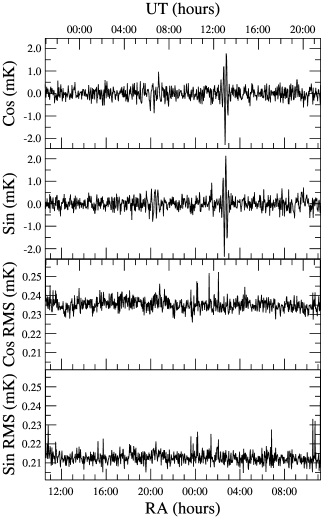
Figure 1: A single interferometer data file at +41°declination, covering just over 24 hours. Basic processing steps, such as calibration and correction for the error in correlator phase quadrature, have been performed. Fringes are just visible at the Galactic plane crossing around 20 hours RA. The feature near 13:00 U.T. is accounted-for by off-axis pick-up of emission from the Sun.

3 Basic Data processing

3.1 Calibrating the raw data

As a first step in the analysis, baselines are subtracted from the CAL-off cosine and sine data and any departure from the quadrature between the sine and cosine data of both the CAL-off and CAL-on records is corrected. On the time-scale it takes to carry out a single 30-second integration cycle, the amplitude and phase response of the instrument can be considered unchanged. By carrying out a complex division of the CAL-off data by the CAL-on data all variations in instrumental performance cancel and calibrated data in units of the amplitude of the CAL signal are obtained. These data are then converted to physical units by multiplying by the measured amplitude of the CAL signal (Section 4). The procedures for removing the baselines and correcting the quadrature will now be outlined.

3.1.1 Baseline removal

The raw CAL-off data contain a small offset of amplitude $\sim$ 1 mK. Daily variations in this offset will appear as extra noise in the stacked data. A high-pass Gaussian filter (i.e. the result of subtracting a low-pass Gaussian filter applied to the data) was used to remove the offset. If the width of this filter is too narrow, higher frequency components of the baseline will remain, thus increasing the noise. Conversely a filter that is too wide will filter out some of the fringes, reducing the astronomical signal. The optimum filter is the one that removes as much of the baseline as possible while leaving the astronomy intact, thus giving the largest signal-to-noise ratio. Observations of the Moon, used for calibration, showed that for typical values of the offset the optimum width of the Gaussian filter was $\sigma$=3$\aas@@fstack{\circ}$2; the reduction in the astronomical signal is negligible and has no effect on the temperature scale as survey and calibration data are scaled by the same factor.

3.1.2 Correcting the quadrature

The output of both channels can be modelled as:

cosine channel: $$A\cos\theta$$

sine channel: $$A(1+\delta)\sin(\theta+\Delta)$$

where $\delta$ is the relative difference in sensitivity between the two channels and $\Delta$ is the departure from quadrature. Provided $\delta$ and $\Delta$ are both small, the data can be brought back into quadrature, with negligible loss of sensitivity using:

$$\left[\begin{array}[]{c}\mbox{cosine}\\ \\ \mbox{sine}\end{array}\right]=\left[\begin{array}[]{cc}1&0\\ \\ -\tan\Delta&{\frac{1}{(1+\delta)\cos\Delta}}\end{array}\right]\left[\begin{array}[]{c}\mbox{cosine ${}^{\prime}$}\\ \\ \mbox{sine ${}^{\prime}$}\end{array}\right]$$ (1)

Moon observations showed $\delta$ to be negligible; while $\Delta$ was found to be 6$\aas@@fstack{\circ}$1, small enough to be corrected using equation 1.

3.2 Editing and quality control of the data

After this relative calibration, the data were re-binned into 2 minute (RA) bins and edited to remove periods of bad weather, spikes and times when the Sun may have contaminated the data. All data points outside a $\pm$650 $\mu$K range ($\sim$3 times the instrumental RMS value) were removed. A visual inspection was carried out and any regions of data with more than $\sim$30 per cent of the points deleted were discarded.

Every 10 days data were stacked, combining all points with the same UT; with this stacking only features due to the Sun will remain in the data. The positions of these features were noted and these areas were deleted in the original data files used to make that stack. Any solar features below the noise in a 10-day UT stack can be neglected as any signals not fixed in RA will be smeared out in the final RA stacks. For most of the year only the midday Sun transit was visible, so only data within $\pm$1 hour of this feature were removed. The exception to this was around mid-summer when all data within $\pm$8 hours of the Sun transient were deleted.

In a single day, with the exceptions of the midday Sun crossing and the Cygnus region in the Galactic plane, the noise is much greater than any astronomical signal. Consequently each data point should be drawn from a normal distribution with a sigma equal to the RMS record which contains information on time-scales less than 30 seconds. Spikes, weather and variations in the offset which occur on large time-scales result in data points with a larger scatter than their RMS records suggest.

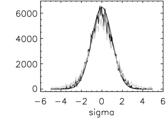
Figure 2: The statistics of the data. This plot is a histogram of 12 days of data divided by their RMS records. The gray and black lines are the unedited and edited data respectively, while the smooth line is the expected $\sigma=1$ Gaussian distribution.

Fig. 2 shows a histogram of the distribution of data points, normalized by dividing through by the mean RMS level. The darker and lighter curves correspond to the edited and unedited data respectively (in both cases the Cygnus region RA=20^h30^m$\pm$ 1^hand the Sun transit have been removed from the data). The smooth line shows the expected distribution if the noise in the data was accurately reflected in the RMS record. This measures noise on timescales $<30\,$s, and is dominated by receiver noise. Both curves follow normal distributions showing that all experimental errors are Gaussian; however the unedited data have a broader distribution showing the effects of weather and other sources of additional noise. The distribution of the edited data is close to the expected curve demonstrating that the data have been edited properly and are limited by system noise alone.

3.3 The stability of CAL

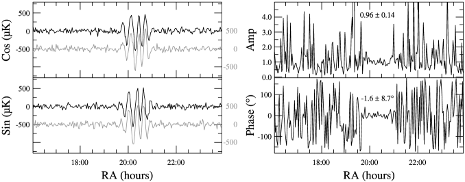
Figure 3: The stability of CAL. The two stacks shown on the left (April/May 1997 in black and August 1997 grey) correspond to approximately 20 days each. On the right is shown the complex division of these two stacks over the Cygnus region (RA=20^h00 to 20^h45), where the signal is much larger than the noise. The amplitude is $\sim$1 and the phase $\sim$0° showing that there has been no change in the Cygnus region, and hence in the amplitude and phase of CAL (see main text).

The data from individual scans, following the processing steps outlined above, will be collected together in a 24-hour stack. The value at each RA position in the stack is given by the mean value at that RA from the contributing scans. This procedure relies on the CAL source being stable. Variations in the amplitude of CAL would increase the noise in the data, and changes in phase by more than a few degrees, as well as averaging out the noise, would smear out the astronomical signal when the data are stacked. To check the stability of CAL, two independent stacks were made, one using data from April/May 1997 and the other using data from August 1997. In areas where the astronomical signal dominates over the noise, the result of the complex division of one of these stacks by the other should have an amplitude of 1 and a phase of 0° if CAL is perfectly stable. Using the Cygnus region shown in Fig. 3 as an astronomical reference it was demonstrated that on a time-scale of 14 weeks CAL is stable to approximately 4 per cent in amplitude and 2° in phase. This process was repeated using pairs of stacks made from data taken at epochs separated by 5 weeks and 6 months. On the 5-week time-scale CAL was stable to better than 3 per cent in amplitude and 2° in phase, while on the 6 month time scale the values were 5 per cent and 4° respectively. These results show that CAL is highly stable and that data taken many months apart can be stacked with negligible error.

3.4 The Dec=+41° stack.

A total of 100 days of usable data were collected at Dec=+41°. These were combined into the stack shown in Fig. 4. The number of observations at each RA varies between 127 and 60 due to the editing out of the Sun. The RMS at each RA is that expected from the RMS on a good day divided by the square root of the number of days of data at that RA, further demonstrating the effectiveness of our editing. The RMS values of the cosine data are marginally higher than the sine data. We attribute this to the asymmetric nature of the sine fringes being slightly better at cancelling atmospheric noise than the symmetric cosine interferometer pattern.

One feature that stands out is the Cygnus region between RA=19^h30^mand 21^h30^m. When plotted in amplitude and phase, two peaks at RA=20^h18^m and 20^h40^m are clearly distinguishable. Similar peaks can be seen in our 5 GHz survey of the same region (Asareh 1997). Most of this observed structure is due to diffuse Galactic free-free emission; however the radio galaxy Cygnus A (RA=19^h57^m Dec=40° 36^′), which has an expected amplitude at Dec=41°of 200$\mu$K, can just be distinguished as the slight bulge on the low RA side of the Cygnus region.

4 Temperature calibration

The amplitude of the CAL signal was measured by the observation of known astronomical sources and also by using hot and cold loads. Astronomical calibration is more robust than calibration based on the response to hot/cold loads as it automatically takes into account systematic errors such as the efficiency of the horn feeds and any attenuation in the atmosphere. Furthermore with practical hot loads allowances must be made for saturation of the receivers. Conversely, astronomical calibration is limited by the shortage of accurate data for suitable sources at high frequencies. However, an error in the assumed flux of a calibration source can be easily corrected, whereas the systematic errors occurring with hot/cold load calibration cannot. As a result CAL was measured using astronomical calibration and calibration with hot/cold loads was used as an additional check.

The large ($\sim 2$°$\times 5$°) size of the primary beam of the interferometer results in low sensitivity to point sources, so only the brightest point sources can be used as astronomical calibrators. At 33 GHz the three brightest sources in the sky are the Sun, the Moon and Tau A (the Crab nebula), all of which are small in comparison to our beam size. Of these, the Sun is too bright, causing saturation of the receivers, making it unsuitable as a calibrator. By contrast, observations of Tau A showed that it had a peak amplitude only $5-6$ times the noise in a 2-minute integration meaning that many days of observations would have to be used in order to obtain an accurate calibration. As is shown below, the power received from the Moon corresponds to an antenna temperature in the range 2–4 K, which is less than half the power received from the sky ( $\sim$ 10 K due to the CMB and the atmosphere) and so saturation of the receivers is not a significant factor. However a 2–4 K signal is large enough to give signal-to-noise ratios of $\sim$6000 in a single observation. Consequently the Moon was used as our primary astronomical calibrator and observations of Tau A were used to confirm the calibration obtained.

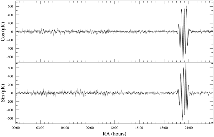
Figure 4: The stack of the data collected at Dec=+41°. The diagram shows the cosine and sine visibility data. The MEM-reduced data stack (heavy line) is plotted over the basic 2-minute data stack (light line).

4.1 Calibration using the Moon

The Moon was modelled as a uniform disk of radius $r_{\rm\tiny Moon}$ and a 33 GHz brightness temperature, $T_{\rm b}$ given by:

$$T_{\rm b}=214+36\cos(\phi-\epsilon)\>\>\mbox{K}$$ (2)

where $\phi$ is the phase of the Moon (measured from full Moon) and $\epsilon$ = 41° is a phase offset caused by the finite thermal conductivity of the Moon (Hagfors 1970). The expected antenna temperature, $T_{\rm E}$, can then be found by integrating over the disk of the Moon, multiplied by the normalized interferometer beam function:

$$T_{\rm E} = \frac{T_{\rm b}}{2\pi{\mbox{$\sigma_{\!{\rm\tiny RA}}$}}{\mbox{$\sigma_{\!{\rm\tiny Dec}}$}}}$$

$$\times \int_{0}^{2\pi}\!\!\!\!\!\int_{0}^{\mbox{$r_{\rm\tiny Moon}$}}\!\!\!\!\!\!\!\!\!\!\exp\left({-\frac{x^{2}}{2{\mbox{$\sigma_{\!{\rm\tiny RA}}$}}^{2}}}{-\frac{y^{2}}{2{\mbox{$\sigma_{\!{\rm\tiny Dec}}$}}^{2}}}\right)\;\cos\left(\frac{2\pi x}{f}\right)\;{\rm d}\Omega$$

where $x=\theta\cos\phi$ and $y=\theta\sin\phi$. $\sigma_{\!{\rm\tiny RA}}$ and $\sigma_{\!{\rm\tiny Dec}}$ are the RA and Dec beam sigmas and $f$ is the fringe spacing (see Section 2).

Regular observations of the Moon were made and the data were processed as described in Section 3. For each observation, equation 4.1 was evaluated numerically and an amplitude for CAL found so that the amplitude of the Moon in the processed data was the same as the predicted value. Using 14 observations of the Moon, an average amplitude for CAL of 15.2$\pm$1.0 K was found. The error is made up from a 3.4 per cent error in the measurements and an estimated 6 per cent in the data presented by Hagfors. A small measurement error in beam area, such as $\sim 4$ per cent, would not affect the overall calibration, since astronomical signals would be re-scaled by the same factor as the Moon calibration. Fig. 5 shows our observations and how the measured brightness temperatures of the Moon changed with phase.

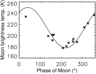
Figure 5: Measured value of the brightness temperature of the Moon. Each of the observations has been calibrated using CAL=15.2 K. The solid line is the prediction of the model based on data given by Hagfors (1970): $T_{b}=214+36\cos(\phi-41)$ in Kelvins. Phase is measured from full Moon.

4.2 Calibration using Tau A

Tau A (the Crab Nebula) is a supernova remnant $6^{\prime}\times 4^{\prime}$ in diameter. Using the model of Baars et al. (1977) and taking into account a secular decrease of 0.166 per cent per year (Aller & Reynolds 1985), at the epoch of observation (1997) Tau A has a 32.5 GHz flux density of 356$\pm$40 Jy. The measured primary beam-shape of the interferometer was used to calculate an effective area for each antenna of the interferometer, and this was used to convert the flux density of Tau A into an antenna temperature. For an unpolarized source it was calculated that the interferometer has a sensitivity of $7.07\,{\rm~{}\mu KJy}^{-1}$, so taking into account a 6.6 % polarization of Tau A at position angle 150°(Mayer & Hollinger 1968) the interferometer $E$ vector at PA=90° should observe Tau A to have an amplitude of 2.51$\pm$0.28 mK.

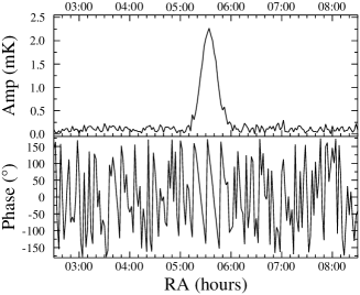
Figure 6: A stack of 12 days of data at Dec=+22$\aas@@fstack{\circ}$0, showing Tau A in amplitude and phase. The amplitude of the peak is 2.51$\pm$0.09 mK assuming a flux density of 356 Jy.

Twelve days of observations at Dec=+22.0° were processed and combined to produce the stack shown in Fig. 6. The measured amplitude of Tau A was found by fitting a Gaussian beam-shape to the data, giving a value for CAL of 16.9$\pm$1.9 K. Although this result is somewhat higher than the value found using the Moon, the two results are consistent within the error.

5 The maximum entropy reconstruction

The stack shown in Fig. 4 has data points every 2 minutes in RA. At Dec=+41° the interferometer beam pattern is $\sim$20 minutes wide so there are $\sim$10 independent points per resolution element in each of the cosine and sine channels. By reducing the number of independent points in each resolution element to 1, improvements to the signal-to-noise ratio of the order of $\sim\sqrt{10}$ should be possible. Simple averaging cannot be used to do this, as positive and negative lobes would cancel. However by de-convolving the data with a technique such as the maximum entropy method (MEM, Gull 1989) and then re-convolving the result with the interferometer beam pattern, it is possible to obtain one independent point per resolution element. The MEM algorithm described in Maisinger et al. (1997) was used to simultaneously deconvolve cosine and sine data, using beam shapes of $\exp[-{\rm RA}^{2}/2{\mbox{$\sigma_{\!{\rm\tiny RA}}$}}^{2}]\cos(2\pi{\rm RA}/f)$ for the cosine channel and $\exp[-{\rm RA}^{2}/2{\mbox{$\sigma_{\!{\rm\tiny RA}}$}}^{2}]\sin(2\pi{\rm RA}/f)$ for the sine channel. Here $\sigma_{\!{\rm\tiny RA}}$and $f$ must be corrected to declination +41°. The MEM-processed Dec=+41° stack can be seen in Fig. 4.

5.1 Errors in the MEM reconstruction

The MEM technique does not determine errors; we use Monte Carlo techniques to make an estimate of the error in the MEM reconstruction using different signal-to-noise ratios. These simulations were generated from a sum of cosines which populate the spatial frequencies to which the interferometer is sensitive, namely

$$\phi=\sum_{i=5}^{300}\cos[2\pi\frac{\rm RA}{i/10}+\theta]$$ (4)

where $\theta$ is a random phase between 0 and $2\pi$. These were convolved with the interferometer beam pattern to produce a noise-less sky which was normalized to 10 $\mu$K RMS. White noise with a known RMS was added to create data with signal-to-noise ratios between 1 and 5.

Two example simulated data sets are shown in Fig. 7. In the upper trace 10 $\mu$K (RMS) noise has been added (a signal-to-noise ratio of 1:1). These simulated data were de convolved using the same parameters as those used for the real data. The MEM reconstruction reproduces the noiseless signal well. In the second case 30 $\mu$K noise has been added. This time the difference between the noiseless data and the reconstruction is larger, but the process is still reproducing real features from the data, despite the high noise level.

The MEM process outlined in Maisinger et al. (1997) also requires the parameters $m$ and $\alpha$ which are respectively the default value for the de convolved sky in the absence of any information, and a regulating parameter which changes the relative weights given to fitting the de convolved sky to the data, and maximising the entropy. As indicated in Maisinger et al. , varying $m$ and $\alpha$ by up to 2 orders of magnitude produced no noticeable change in the re-convolved skies, thus demonstrating the reliability of MEM.

The RMS of the difference between each re-convolved result and the corresponding noise-less observed signal was calculated. This process was repeated over 100 skies. The average RMS error in the re-convolved results plotted against the RMS noise added to the simulated data can be seen in Fig. 8. The best-fit quadratic line to this graph was used to estimate the errors of the data in Fig. 4 from the errors in the Dec=+41° stack. On average MEM decreased the errors by a factor of 3.4 as expected from the number of 2-minute points per resolution element. By de-convolving the simulated skies containing 10 $\mu$K of signal and 10 $\mu$K noise it was shown that using beam widths and fringe spacing up to 5 per cent different to those used to create the fake data had little effect on the re-convolved output from MEM. As the errors in the measured beam-shape are less than 2 per cent, they will have a negligible effect on the output from MEM.

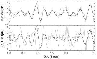
Figure 7: Example sky models used for Monte–Carlo MEM analysis. The noiseless sky model, shown by dashed lines, has an RMS signal level of 10 $\mu$K (comparable with expected CMB levels). Different RMS levels of noise are added – in these examples: (a) 10 $\mu$K and (b) 30 $\mu$K. The resulting simulated noisy data are shown with faint lines. In each case a MEM analysis is performed. The resulting reconstructed sky signals are shown with solid lines.

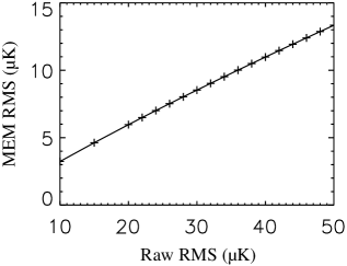
Figure 8: The RMS noise in the MEM-processed data over the one beam width resolution element plotted against the RMS noise in the 2-minute data stack. Each point was found by de-convolving 100 simulated skies.

5.2 Evidence for structure

The MEM-processed data show a good match to the unprocessed stack, especially over the Cygnus region. The average RMS error on each point, as calculated using the above Monte Carlo simulations, is 7.1 $\mu$K and from 12^h to 19^h the RMS on some points is lower than 6.0 $\mu$K. Many features in Fig. 4 are real at a greater than 2-sigma level and some (for example at 11^h RA) are real at a 6-sigma level. The origin of these features is discussed in Section 7 while their RMS amplitude can be estimated by the quadrature subtraction of the uncertainty in the data from the RMS scatter of the data points (as estimated from Fig. 4). Between 8^h00 and 19^h30 RA the cosine and sine data have RMS scatters of $12.2\pm 1.4\,{\rm\mu K}$ and $12.1\pm 1.4\,{\rm\mu K}$ respectively. The errors in these scatters take into account that neighbouring points are not independent. Over the same region the corresponding averages of the RMS records are $6.9\pm 1.0\,{\rm\mu K}$ and $6.8\pm 1.0\,{\rm\mu K}$ so the observed astronomical signal has a RMS amplitude of $10.1\pm 1.8\,{\rm\mu K}$. Using the window function from Section 6 and assuming that the power spectrum of the sky fluctuations is flat, it can be shown that this corresponds to an intrinsic fluctuation amplitude of $\Delta T_{\ell}=57\pm 10\,{\rm\mu K}$. A more quantitative measurement of this structure using Maximum Likelihood follows.

6 Likelihood analysis

Methods based on the likelihood function have been used extensively in the analysis of CMB data (see for instance Hancock et al. 1997). The method considers the statistical probability distribution of the CMB signal, and takes into account how the observing strategy, experimental configuration, etc. modifies the statistical properties of the sky signal. In standard models, the CMB fluctuations are described by a Gaussian multi-normal random field, which is fully described by its power spectrum or alternatively by the two-point correlation function. In this case the likelihood function follows a multi-normal distribution with the covariance matrix composed of two terms due to the signal and noise respectively: $\bf C=S+N$. In our case the data consist of a set of differences in temperature of the cosine and sine channels along with their error bars binned in 2-minute bins in RA. For the noise correlation matrix, the only non-zero terms are those on the diagonal, as the instrumental noise is uncorrelated from point to point.

We have assumed that the CMB signal has a flat power spectrum ($\Delta T_{\ell}\equiv\sqrt{l(l+1)C_{\ell}/2\pi}$ constant) over the range covered by the window function of the instrument, and then the expected two-point correlation between a pair of points $i$ and $j$ separated by an angle $\theta_{ij}$ is given by

$$\left<T_{i}\cdot T_{j}\right>\ = \exp\left(\frac{-\theta_{ij}^{2}}{4\sigma^{2}}\right)\cos\left(\frac{2\pi\theta_{ij}}{f}\right)\frac{\Delta T^{2}_{l}}{2}$$ (5)

$$\times \sum_{l_{1}}^{l_{2}}\frac{2l+1}{l(l+1)}W_{\ell}(\theta_{ij})$$

$W_{\ell}(\theta_{ij})$ being the window function of the experiment which defines the response of the instrument to a given multipoles or angular scale. The computation of the window function of an interferometer like the one analyzed here is not straight-forward. We adapted the method of Muciaccia, Natoli and Vittorio (1997) to decompose the beam configuration into spherical harmonics, which can then be used to form the window function. The resulting function (see Fig. 9) can be fitted by:

$$W_{\ell}(0)=0.677\exp(-(\ell-109)(\ell-110)/730).$$ (6)

This defines the range of sensitivity to be $l\sim 109\pm 19$. We use this to calculate the expected excess variance in the data for some theoretical model prediction on band power [Bond 1997]. Starting with the convolved sky covariance function at zero lag, which is the same as the data variance

$$C_{m}(0)\equiv\frac{1}{4\pi}\sum_{\ell}{(2\ell+1)C_{\ell}W_{\ell}(0)},$$ (7)

we can substitute for $C_{\ell}$ from the definition of band power to obtain the ratio of filtered to non-filtered variance

$$C_{m}(0)/\Delta T_{\ell}^{2}=\frac{1}{2}\sum_{\ell}\frac{(2\ell+1)}{\ell(\ell+1)}W_{\ell}(0)=32.5$$ (8)

For the likelihood analysis it is necessary to construct the expected theoretical covariance matrix which corresponds to carrying out the above procedure for non-zero lag window functions. As the window is narrow we can just use the beam autocorrelation function and normalize it to the ratio found above for zero lag.

Figure 9: The window function of the interferometer.

6.1 The Galactic cut

To locate regions free of significant Galactic emission, 48 intervals of 5 hours in RA each stepped by 30 minutes in RA were analysed using the likelihood function. It was found that the amplitude of the detected signal was at a low stable level in the range RA=8.0–19.5 hours, indicating a low level of foreground contamination over this region showing no change with Galactic latitude. Further indications that this region is free from foreground contamination are discussed in Section 7.2. It is worth noting that when data from the sine channel for the region RA=8-11 hours are included in the analysis there is marginal evidence (at the one-sigma level) of a slightly larger signal as compared with the results in RA=11.0–19.5 hours and those of the cosine channel; this effect could be due to some minor atmospheric residual in this channel (see Section 3 and below).

6.2 The results

A likelihood analysis of each channel over the RA=8.0–19.5 hour range gave $\Delta T_{\ell}=49^{+12}_{-11}$ and $37^{+18}_{-18}$ $\mu$K (68 % C.L.) for the cosine and sine channels respectively. The larger uncertainty for the sine channel reflects the shape of the likelihood function which has lower peak and is broader than the likelihood function of the cosine channel, however the signals detected in each channel are consistent at the one-sigma level. An additional test of the consistency and repeatability of these results was carried out by the likelihood analysis of two independent data stacks, one formed from the first 50 days of data used to make the main stack and another formed from the remaining data. The results for each sub-stack are in agreement with each other and with the above results obtained when the full data of each channel are analyzed.

The best estimation of the signal present in our data comes from the joint analysis of both channels. When data from both the cosine and sine channels are analyzed together building the joint likelihood function the signal detected is $\Delta T_{\ell}=45^{+13}_{-12}$ $\mu$K at the 68 % C.L. This indicates not only that the amplitude of the signal detected in each channel is in agreement, but also that the signal detected by both channels comes from the same structures.

With a limited sky coverage consideration of the “sample variance” [Scott, Srednicki & White 1994] is crucial to an understanding of the quoted errors. To quantify this contribution we integrate the square of the telescope two-point correlation function over the survey area (equation 4 of Scott et al.). For our single 11.5-hour RA strip ($\sim$35 independent beam widths) the contribution is 20.7 per cent, or $8.9\,{\rm\mu K}$. In comparison the receiver noise contribution is approximately $5.2\,{\rm\mu K}$, added in quadrature (see Table 1). The maximum likelihood error is slightly larger than expected, possibly due to a contribution from weather effects. The effect of finite sky coverage represents the majority of the error in our determination of the amplitude of CMB fluctuations. Additional observations at other declinations, which are being conducted now, will increase our sky coverage, significantly reducing this uncertainty.

The contributions of weak point sources and Galactic emission, which would add in quadrature to the $\Delta T_{\ell}$ arising from the CMB, are discussed in sections 7.1 and 7.2, below. Since these could lead to a small over-estimate in $\Delta T_{\ell}$, we extend the negative error bar slightly, as given in Table 1.

Table 1: Contributions to the error in $\Delta T_{\ell}$. The receiver noise and sampling error add in quadrature, accounting for most of the maximum liklihood error. Weak point sources and Galactic emission would contribute in quadrature to $\Delta T_{\ell}$ and so can only have lead to a small over-estimate. This is allowed-for by a small extension to the negative error on $\Delta T_{\ell}$. The survey is referenced to the Moon temperature, with the calibration uncertainty given.

Receiver noise		$\pm$	$5.2$	${\rm\mu K}$
Sampling error	(20.7 %)	$\pm$	$8.9$	${\rm\mu K}$
Weak point sources	($\Delta T\la 8\,{\rm\mu K}$)	$-$	$0.5$	${\rm\mu K}$
Galactic free-free	($\Delta T\la 2\,{\rm\mu K}$)	$-$	$0.05$	${\rm\mu K}$
Maximum Likelihood error			${}^{+12.5}_{-12.0}$	${\rm\mu K}$
Calibration		$\pm$	$6.6$	%

7 Foregrounds

7.1 Point Sources

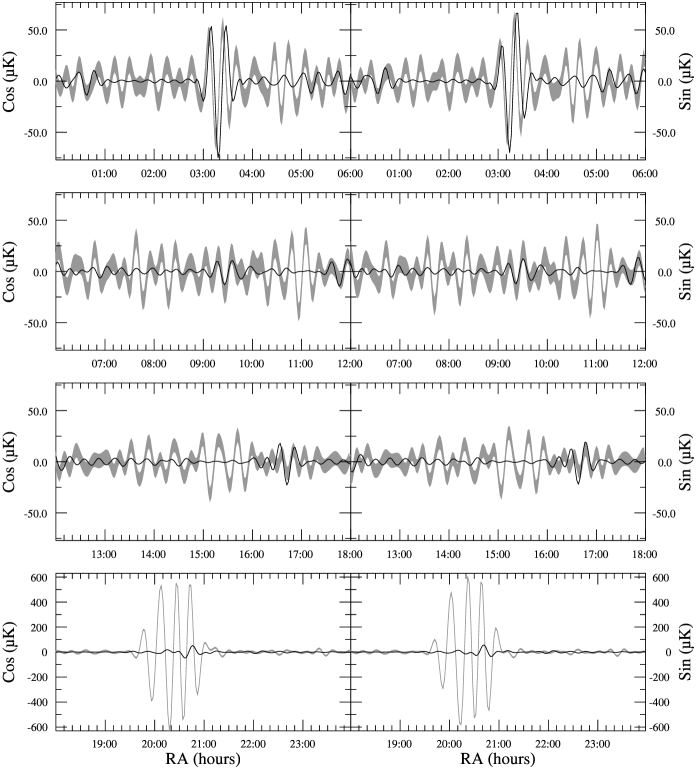
Figure 10: The contribution of point sources with predicted S(33GHz)$\geq$0.2 Jy in the field of the Dec=+41° scan. The black lines represent the predicted point source contribution, while the grey lines are the MEM-fitted data with their 1$\sigma$ errors.

Only the strongest sources at 33 GHz have reliably measured flux densities since no large-area survey is available at this frequency. Furthermore, many of the strongest sources have flat spectra and are time-variable. The 5 sources with S(33 GHz)$\geq$ 2 Jy within the 4^∘-wide strip centred on Dec=41° are monitored on a continuous basis in the Metsahovi 22 and 37 GHz programme (Teräsranta et al. 1992). They are listed in Table 2. The sources are all variable; Dr. Harri Teräsanta has kindly provided data covering the observing period of the present CMB survey.

Table 2: Sources within a 4^∘-wide Dec strip centred on +41°.

Name	RA2000	Dec2000
3C 84	03h  19m  48s	+41° 30′ 42″
DA 193	05h  55m  31s	+39° 48′ 49″
4C 39.25	09h  27m  03s	+39° 02′ 21″
3C 345	16h  42m  59s	+39° 48′ 37″
BL Lac	22h  02m  43s	+42° 16′ 40″

A limited amount of 33 GHz data on other (weaker) sources is available in the Kuhr et al. (1981) Catalogue. The highest radio frequency survey covering the sky around Dec=+41° is the 4.85 GHz Green Bank survey (Gregory et al. 1996). Those sources with S(5 GHz)$\geq$0.2 Jy lying within Dec=41°$\pm$3° were selected as possible contributors to the 33 GHz point source background. The Kuhr catalogue gives measured flux densities in the range 14–37 GHz for 90 per cent of the Green Bank sources with S(5 GHz)$\geq$1 Jy. For these, a reliable 33 GHz flux density could be derived. For the remaining sources with S(5 GHz)$\geq$0.2 Jy, S(33 GHz) was estimated using the spectral index between the flux density given in the 1.4 GHz NVSS Catalogue (Condon et al. 1989) and that given in the Green Bank 5 GHz survey, assuming a spectrum of the form $S\sim\nu^{\alpha}$ where $\alpha$ is the spectral index. Where no matching 1.4 GHz source was found, a conservative index of -0.1 was assumed.

The 33 GHz flux densities of the sources identified above were then convolved with the two-dimensional interferometer beam pattern centred on Dec=+41°. The flux densities were converted to antenna temperature using the factor 7.07$\mu$K Jy^-1 calculated in Section 4.2. The predicted contribution of these point sources is compared with the MEM-reduced observed data in Fig. 10. The sources 3C84 and 3C345 show good matches to the observed data. Over the Galactic plane regions (RA=5^h30^m – 6^h30^m and 19^h30^m – 21^h30^m) flux predictions for point sources were difficult as most surveys avoid these crowded areas. In these regions we expect most of the observed structure to be due to Galactic sources and, as we have excluded these regions from our analysis to determine the CMB structure, the contribution from both Galactic and extra-galactic sources is irrelevant.

Excluding the Galactic regions and the 5 strongest point sources, the RMS of the MEM-reduced data is approximately 10 times that predicted from discrete point sources alone. As a check that the likelihood results do not depend strongly on the point source prediction, the above likelihood analysis was repeated with and without the subtraction of point sources. It was found that with the point sources subtracted the result of the analysis of the cosine and sine data together gave $\Delta T_{\ell}=43^{+12.5}_{-11.5}\,{\rm\mu K}$ as compared to $\Delta T_{\ell}=45\,{\rm\mu K}$ without, thus demonstrating that point source contribution is not a major concern for the data presented here.

Although it has been shown that the discrete resolved point sources do not contribute significantly to our observed value of $\Delta T_{\ell}$, it is necessary to quantify the contribution due to a foreground of unresolved point sources. The expected RMS for a random distribution of such sources varies with frequency and angular scale. On scales of 1$\aas@@fstack{\circ}$6 and at a frequency of 33 GHz, Franceschini et al. (1989) predict that unresolved point sources should have $\Delta T/T$ $\approx 3\times 10^{-6}$ corresponding to $\Delta T=8\,{\rm\mu K}$. This would add a contribution in quadrature, accounting for approximately $0.5\,{\rm\mu K}$ of the total. Unresolved point sources are therefore unlikely to make a significant contribution to our estimate of $\Delta T_{\ell}$. We may allow for this component by extending the negative error range by $0.5\,{\rm\mu K}$, giving $\Delta T_{\ell}=43^{+12.5}_{-12.0}\,{\rm\mu K}$, as given in Table 1.

7.2 Diffuse Galactic emission

An indirect estimate of the amplitude of the diffuse Galactic component in our data can be computed using the results obtained in the same region of the sky by the Tenerife CMB experiments (Gutiérrez et al. 1998). At 10.4 GHz and on angular scales centred on $\ell=20$ the maximum Galactic component was estimated to be $\leq 28\,{\rm\mu K}$. Assuming that this contribution is entirely due to free-free emission and a conservative Galactic spatial power spectrum of $\ell^{-2.5}$ (Lasenby 1996, Davies & Wilkinson 1998), the predicted maximum Galactic contamination in the data presented here is $\leq 2\,{\rm\mu K}$, less than 5 per cent of our measured value. Any such contribution would add in quadrature to that from the CMB, accounting for approximately $0.05\,{\rm\mu K}$, which is insignificant. The true make-up of the Galactic foreground emission detected at 10.4 GHz most probably has a steeper average index than this, so the contribution to our result will be even lower than stated.

Several experiments [Kogut et al. 1996, De Oliveira-Costa et al. 1997, Leitch et al. 1997] have detected an “anomalous” microwave emission, correlated with 100-${\rm\mu m}$ thermal emission from interstellar dust. It has been argued [Draine & Lazarian 1998] that spinning dust grains containing $\sim 10^{2}-10^{3}$ atoms might be responsible. Our survey region is in an area of low 100-${\rm\mu m}$ emission, but even so a contribution from spinning dust comparable to that of free-free emission is possible. Again, such a contribution would add in quadrature to the CMB, and even a level as high as $15\,{\rm\mu K}$ would account for only $3\,{\rm\mu K}$ of our measurement.

8 Conclusions and the future programme

We describe in this paper the results from the first high sensitivity data stack taken with the new Jodrell Bank – IAC 33 GHz interferometer in a strip at Dec=+41°. By using the MEM technique it has been possible to reduce the RMS noise in each 5° RA beam width of the stack to $6\,{\rm\mu K}$. The source 3C84 is clearly seen in the data at the level expected from its monitored intensity at Metsahovi. All the other individual sources are weaker than the measured signals in the raw data as shown in Fig. 10. Furthermore, arguments are presented in Section 7.2 that the RMS Galactic contribution, neglecting dust, is $\Delta T\leq 2\,{\rm\mu K}$, and is therefore negligible. Thus, apart from the region of the stack around 3C84 (RA=3^h20^m) and the strong Galactic plane crossing (RA=19^h.5–21^h.5) the stack shows significant CMB signals over the entire RA range. Many of these CMB features have amplitudes 4–5 times the RMS noise in the 5° beam width. When corrected for dilution in the beam of the interferometer these features have a sky brightness temperature of $\sim 100\,{\rm\mu K}$.

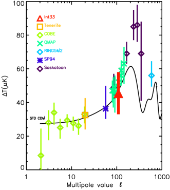
Figure 11: The C_ℓ versus $\ell$ plot of recently published data on CMB anisotropies including the present result (shown by the heavy line) of $\Delta T_{\ell}=43^{+12}_{-12}{\rm\,\mu K}$ at $\ell=109\pm 19$.

The value of the intrinsic CMB fluctuation amplitude derived from the present observations at high Galactic latitudes is $\Delta T_{\ell}=43^{+12.5}_{-12.0}\,{\rm\mu K}$. In the maximum likelihood analysis only one 11.5-hour long RA strip is used. This leads to a sampling error of approximately 21 per cent, which is the main contributor to the $\sim 25$ per cent uncertainty of our result. The remainder is due to receiver noise. Clearly the major improvement in an estimate of $\Delta T_{\ell}$ will come from the coverage of a larger area of the sky at the present or better receiver sensitivity. Further observations are being undertaken at adjacent declinations of +39$\aas@@fstack{\circ}$8 and 42$\aas@@fstack{\circ}$2 in addition to the full RA range at Dec=+41°. These should increase the area covered by a factor of 4 which will reduce the sampling error to approximately 10 per cent, comparable with the receiver noise contribution, reducing the total error to $\sim$ 15 per cent. In addition to the quoted error there is a calibration uncertainty of $\pm 6.6$ per cent, arising mostly from uncertainty in the Moon temperature. Future improvements to the calibration are possible.

This result obtained at 32.5 GHz and at high Galactic latitude may be compared with others at similar values of $\ell$ but made at different frequencies and Galactic environments. Our best estimate is $\Delta T_{\ell}=43^{+12.5}_{-11.5}\,{\rm\mu K}$ in the range $\ell=109\pm 19$. Two such recent measurements have been made in the North Celestial Pole (NCP) region. One is the Saskatoon experiment (Netterfield et al. 1997) at 26–46 GHz which found $\Delta T_{\ell}=49^{+8}_{-5}{\rm~{}\mu K}$ at $\ell=87$; there is a further 15 per cent calibration uncertainty in this result. The other is QMAP (De Oliveira-Costa et al. 1998) which at 30 GHz found $\Delta T_{\ell}=47^{+6}_{-7}\,{\rm\mu K}$ at $\ell=80$ and $\Delta T_{\ell}=59^{+6}_{-7}\,{\rm\mu K}$ at $\ell=126$ while at 40 GHz it found $52^{+5}_{-5}\,{\rm\mu K}$ at $\ell=111$. At the South Celestial Pole (SCP), the SP94 (Gundersen et al. 1995) estimated $\Delta T_{\ell}=36^{+13}_{-6}\,{\rm\mu K}$ at $\ell=60$ and Python (Platt et al. 1997) obtained $\Delta T_{\ell}=60^{+15}_{-13}\,{\rm\mu K}$ at $\ell=87$. These values, along with the result reported here and other recently published values, are plotted on Fig. 11. All these results together strongly indicate a significant increase in fluctuation amplitude at $\ell\sim 100$ compared with the COBE value of $\Delta T_{\ell}=30\,{\rm\mu K}$ at $\ell\sim 10$, thereby arguing for the existence of the first Doppler peak.

Another future contribution by the interferometer will be observations on a scale of $\sim$ 1° ($\ell\sim$ 200) with a baseline of 304 mm in place of the present 152 mm. Such observations will enable us to sample the first acoustic peak. The values of $\Delta T_{\ell}$ at $\ell=100$ and 200 will thus be directly compared using the same instrument and the same calibration methods, enabling a better estimate to be made of the width and amplitude of the first peak.

9 Acknowledgements

This work has been supported by the European Community Science program contract SCI-ST920830, the Human Capital and Mobility contract CHRXCT920079 and the UK Particle Physics and Astronomy Research Council. AW acknowledges the receipt of a Daphne Jackson Research Fellowship, SRD and DLH PPARC Postgraduate Studentships. We thank Dr.H.Teräsranta for providing data on point sources at 22 and 37 GHz.

References

- [] Aller, H. D., Reynolds, S. P., 1985, ApJ, 293, L73
- [] Asareh, H. 1997, PhD thesis, University of Manchester
- [] Baars, M. W. M., Genzel, R., Pauliny-Toth, I. I. K., Witzel, A., 1977, AA, 61, 99
- [Bond 1997] Bond, J. R., 1997, in Borner, G., Gottlober, S., eds, The Evolution of the Universe : report of the Dahlem Workshop on the Evolution of the Universe, J. Wiley, New York, p. 199
- [] Condon, J. J., Broderick, J. J., Seielstad, G. A., 1989, AJ, 97, 1064
- [Davies & Wilkinson 1998] Davies R. D., Wilkinson A., 1998, in Bouchet F., Tran Thanh Van J., eds, 33rd Recontre de Moriond, Fundamental Parameters in Cosmology, Editions Frontièrs, Gif-sur-Yvette
- [De Oliveira-Costa et al. 1997] de Oliveira-Costa, A., Kogut, A., Devlin, M. J., Netterfield, C. B., Page, L. A., Wollack, E. J., 1997, ApJ, 482, L17
- [] de Oliveira-Costa, A., Devlin, M. J., Herbig, T., Miller, A. D., Netterfield, C. B., Page, L. A., Tegmark, M., 1998, ApJ, 509, L77
- [Draine & Lazarian 1998] Draine, B. T., Lazarian, A., 1998, ApJ, 494, L19
- [] Franceschini, A., Toffolatti, L., Danese, L., De Zotti, G., 1989, ApJ, 344, 35
- [] Gregory, P. C., Scott, W. K., Douglas, K., Condon, J. J., 1996, ApJS, 103, 427
- [] Gull, S. F., 1989, in Skilling, J., ed., Maximum Entropy and Bayesian Methods, Kluwer, Dordrecht, p.53
- [] Gundersen, J. O., et al., 1995, ApJ, 443, L57
- [] Gutiérrez, C. M., Rebolo, R., Watson, R. A., Davies, R. D., Jones, A. W., Lasenby, A. N., 1998, Submitted for publication in ApJ
- [] Hagfors, T. 1970, RadSci, 5, 189
- [] Hancock, S., Davies, R. D., Lasenby, A. N., Gutiérrez, C. M., Watson, R. A., Rebolo, R., Beckman, J. E. 1994, Nature, 367, 333
- [] Hancock, S., Gutiérrez, C. M., Davies, R. D., Lasenby, A. N., Rocha, G., Rebolo, R., Watson, R. A., Tegmark, M., 1997, MNRAS, 289, 505
- [] Hancock, S., Rocha, G., Lasenby, A.N., Gutierrez, C.M., 1998, MNRAS, 294, L1
- [] Kühr, H., Witzel, A., Pauliny-Toth, I.I.K., & Nauber, U. 1981, AASS, 45, 367
- [Kogut et al. 1996] Kogut, A., Banday, A. J., Bennett, C. L., Gorsky, K. M., Hinshaw, G., Reach, W. T., 1996, ApJ, 460, 1
- [Lasenby 1996] Lasenby A.N., 1996, in Bouchet F., Tran Thanh Van J., eds, 31st Recontre de Moriond, Microwave Background Anisotropies, Editions Frontièrs, Gif-sur-Yvette, astro-ph/9611214
- [Leitch et al. 1997] Leitch, E. M., Readhead, A. C. S., Pearson, T. J., & Myers, S. T., 1997, ApJ, 486, L23
- [] Lineweaver, C.H., 1998, ApJ, 505, L69
- [] Maisinger, K., Hobson, M. P., & Lasenby, A. N., 1997, MNRAS, 290, 313
- [] Mayer, C. H., Hollinger, P.J. 1968, ApJ, 151, 53
- [] Melhuish, S. J., Dicker, S. R., Davies, R. D., Gutiérrez, C. M., Watson, R. A., Davis, R. J., Hoyland, R., Rebolo, R., 1999, Accepted for publication in MNRAS
- [] Muciaccia, P. F., Natoli, P, Vittorio, N., 1997, ApJ, 488, L63
- [] Netterfield, C. B., Devlin, M. J., Jarolik, N., Page, L., Wollack, E. J., 1997, ApJ, 474, 47
- [] Platt S. R., Kovac, J., Dragovan, M., Peterson, J. B., Ruhl, J.E., 1997, ApJ, 475, L1
- [Scott, Srednicki & White 1994] Scott, D., Srednicki, M., White, M., 1994, ApJ, 421, L5
- [] Smoot, G. F., et al., 1992, ApJ, 396, L1
- [] Teräsranta, H., et al., 1992, A&AS, 94, 121
- [] Tegmark, M., 1998, ApJ, 514, L69