Measurement of the solar neutrino capture rate with gallium metal

Abstract

The solar neutrino capture rate measured by the Russian-American Gallium Experiment (SAGE) on metallic gallium during the period January 1990 through December 1997 is $67.2_{-7.0-3.0}^{+7.2+3.5}$ SNU, where the uncertainties are statistical and systematic, respectively. This represents only about half of the predicted standard solar model rate of 129 SNU. All the experimental procedures, including extraction of germanium from gallium, counting of ⁷¹Ge, and data analysis, are discussed in detail.

]

I Introduction

The Sun produces its energy by the nuclear fusion of four protons into an $\alpha$ particle, chains of reactions that yield two positrons and two neutrinos. Since these low-energy neutrinos are weakly interacting, it was assumed that they traverse the Sun and reach the Earth without change. Measurement of the neutrino energy spectrum should thus give information about the conditions under which the nuclear reactions take place in the Sun. All solar neutrino experiments, however, have observed considerably fewer neutrinos than are predicted by detailed models of the physical processes in the Sun that are based on the nuclear reaction chains. As a result of this neutrino deficit, the assumption that the neutrinos are unchanged during their passage from the Sun to the Earth is now seriously questioned. For such transformations to occur neutrinos must have mass, a hypothesis of far-reaching consequences.

The experimental study of solar neutrinos is now over 30 years old. The first experiment, a radiochemical detector based on chlorine [1, 2], observed a capture rate of $2.55\pm 0.17\pm 0.18$ SNU, where 1 SNU = 1 interaction/s in a target that contains $10^{36}$ atoms of the neutrino absorbing isotope. Although different standard solar models (SSM’s) predict somewhat different rates for the chlorine experiment (for example, $7.7^{+1.2}_{-1.0}$ SNU [3, 4] and 7.2 SNU [5]), all such models predict a rate significantly higher than observed.

TABLE I.: Predicted solar neutrino fluxes [4] and their contribution to the Ga capture rate.

	$\nu$	$\nu$ energy	$\nu$ flux	$Gacapture$
Reaction	branch	(MeV)	(cm-2 s-1)	$rate(SNU)$
$p+p{\rightarrow}d+e^{+}+\nu$	$pp$	0–0.42	$(5.94\pm 0.06)\times 10^{10}$	$69.6$
${}^{7}\text{Be}+e^{-}{\rightarrow}^{8}\text{B}+\nu$	7Be	0.38, 0.86	$(4.80\pm 0.43)\times 10^{9}$	$34.4$
${}^{8}\text{B}{\rightarrow}^{8}\text{Be}^{*}+e^{+}+\nu$	8B	0–14.1	$(5.15^{+0.98}_{-0.72})\times 10^{6}$	$12.4$
CNO reactions	CNO	0–1.73	$(1.1\pm 0.2)\times 10^{8}$	$9.8$
$p+e^{-}+p{\rightarrow}d+\nu$	$pep$	1.44	$(1.39\pm 0.01)\times 10^{8}$	$2.8$

For 20 years, until about 1985, the chlorine experiment was the only measurement. This experiment is primarily sensitive to high-energy ⁸B neutrinos with a $\sim 20$% contribution from other sources, mainly ⁷Be. The flux of ⁸B neutrinos is very dependent on the central temperature of the Sun ($T_{\odot}^{24}$[6]). As a result many models were suggested that would slightly suppress $T_{\odot}$ and hence decrease the ⁸B flux significantly. (See Ref. [7] for a description of a large number of such models.) Most of these models, however, run into difficulty with some other measured aspect of the Sun. An alternative solution to this discrepancy could be neutrino oscillations. The Cl experiment operates on the inverse beta decay reaction and thus is only sensitive to electron neutrinos. If the neutrinos were to change flavor on their trip from the solar core to the Earth, the Cl experiment would not observe them.

In the mid 1980s, the Kamioka nucleon decay experiment (Kamiokande) began to measure the solar neutrino flux. This large water Cherenkov detector was originally designed to look for high-energy signals from proton decay. After great effort, the energy threshold was reduced to a level to permit a sensitivity to recoil electrons from ⁸B solar neutrino interactions. The path of the recoil electrons is in the direction of the initial neutrino trajectory, and thus this experiment demonstrated for the first time that neutrinos were coming from the Sun. The measured flux [8] of $(2.80\pm 0.19\pm 0.33)\times 10^{6}$/(cm² s) was less than half of the solar model prediction, and the solar neutrino problem was thus confirmed by a second experiment.

Because the high-energy solar neutrino flux was suppressed, it became very important to also determine the flux of low-energy neutrinos produced in the dominant proton-proton ($pp$) reaction. Exotic hypotheses aside, the rate of the $pp$ reaction is directly related to the solar luminosity and is insensitive to alterations in the solar model. In the early 1990s the Russian-American Gallium Experiment (SAGE) and then the Gallium Experiment (GALLEX) began to publish results. These experiments are based on the neutrino capture reaction ⁷¹Ga$(\nu_{e},e^{-})$⁷¹Ge [9] and have the very low threshold of 233 keV [10]. They are thus sensitive to low-energy $pp$ neutrinos, whose end point energy is 423 keV [11], and provide the only feasible means at present to measure low-energy solar neutrinos. The SAGE result [12] of $66.9^{+7.1+5.4}_{-6.8-5.7}$ SNU with a target of Ga metal and the GALLEX result [13] of $77.5\pm 6.2^{+4.3}_{-4.7}$ SNU with a target of GaCl₃ are both well below the SSM prediction from the Bahcall-Pinsonneault solar model [4] of $129^{+8}_{-6}$ SNU. The insensitivity of Ga to the solar model is seen in the capture rate calculation from the model of Brun, Turck-Chièze, and Morel [5] of 127.2 SNU. The contributions of the components of the solar neutrino flux to the ⁷¹Ga capture rate are given in Table I.

With the four experiments having three different thresholds, one can deduce some information concerning the $\nu$ energy spectral distribution. If one fits the data from all experiments with the neutrino fluxes as free parameters, the best fit is when the $\nu_{\text{Be}}$ flux is greatly reduced whereas there is an appreciable $\nu_{\text{B}}$ flux [14, 15, 16]. This is an apparent paradox as it is difficult to form ⁸B in the Sun without forming ⁷Be.

In 1996 Super-Kamiokande began to take data. This 50 kton water Cherenkov detector is the first high-count-rate solar neutrino experiment. The present result [17] for the ⁸B neutrino flux, assuming that neutrino transformations do not occur, is $(2.44\pm 0.05_{-0.07}^{+0.09})\times 10^{6}$/(cm² s), in agreement with its predecessor.

The purpose of this paper is to summarize all of the SAGE data for the last eight years. It is organized in the same way as the SAGE experiment is carried out: after presenting some general aspects of the experiment, we consider the chemical extraction of Ge from Ga and the subsequent Ge purification. Then we present how the Ge is counted, how ⁷¹Ge events are identified, and how the data are analyzed to give the solar neutrino capture rate. Finally, we consider the sources of systematic uncertainty, give the overall results, and conclude with the implications for solar and neutrino physics.

In an attempt to make the material understandable to the general reader, but still useful to the specialist, each of these subjects is first discussed in a general way, followed by subsections that give more detail. The reader who wants a general overview need only read the beginning of each section. The reader who desires more information regarding a particular subject should read the appropriate subsection.

II SAGE Overview

In this section we give some general information on the location of the experiment, its physical characteristics, and the division of the SAGE data into three experimental periods.

A Baksan Neutrino Observatory

The SAGE experiment is situated in a specially built underground laboratory at the Baksan Neutrino Observatory (BNO) of the Institute for Nuclear Research of the Russian Academy of Sciences in the northern Caucasus mountains. The main chamber of the laboratory is 60 m long, 10 m wide, and 12 m high. It is located 3.5 km from the entrance of a horizontal adit excavated into the side of Mount Andyrchi and has an overhead shielding of 4700 meters of water equivalent. To reduce neutron and gamma backgrounds from the rock, the laboratory is entirely lined with 60 cm of low-radioactivity concrete with an outer 6 mm steel shell. All aspects of the experiment are in this underground area, with additional rooms devoted to chemistry, counting, and a low-background solid-state Ge detector. Other facilities for subsidiary measurements are in a general laboratory building outside the adit.

B Extraction history

The data from SAGE span nearly a decade during which the experiment evolved a great deal. As a result, the data can be naturally divided into several periods characterized by different experimental conditions. Extractions on approximately 30 tons of Ga began in 1988; by late 1989 backgrounds were low enough to begin solar neutrino measurements. The data period referred to as SAGE I began in January 1990 and ended in May 1992 [18]. In the summer of 1991, the extraction mass was increased to nearly 60 tons. The SAGE I data were taken without digitized wave forms and the $L$ peak could not be analyzed because of high electronic noise at low energy. (The decay modes of ⁷¹Ge are described below in Sec. IV.) The solar neutrino capture rate determined from this data were published in Ref. [19].

Within a few months after SAGE I was completed, the experiment was greatly improved with respect to electronic noise. The following period of data, from September 1992 to December 1994, is referred to as SAGE II. It is distinguished by recording of the counter wave form in most runs which makes possible analysis of events in the low-energy $L$ peak.

TABLE II.: Definition of the various segments of SAGE data.

Designation	Included extractions	Comments
SAGE I	Jan. 90 $\rightarrow$ May 92	Rise time from ADP
SAGE II.1	Sep. 92 $\rightarrow$ Oct. 93	Rise time from wave form,
		begin to use $L$ peak
SAGE II.2	Nov. 93 $\rightarrow$ June 94	Ga theft period
SAGE II.3	July 94 $\rightarrow$ Dec. 94	Before Cr experiment
SAGE III.1	Jan. 95 $\rightarrow$ June 95	Some extractions
		during Cr experiment
SAGE III.2	July 95 $\rightarrow$ present	After Cr experiment

During SAGE II, there was a period (which we call SAGE II.2) in which 2 tons of gallium, approximately 3.6% of the total mass, was stolen from the experiment. The gallium was apparently removed in small quantities from November 1993 to June 1994. During this period a prototype gravity wave laser interferometer at BNO detected unapproved transport of materials from underground. After discovery of the theft, all of the gallium was cleaned, additional security controls for access to the gallium were instituted, and SAGE resumed operation. As this period of time has some uncertainty with respect to experimental control, it is singled out for separate treatment, and is not included in our best estimate for the neutrino capture rate.

An experiment using a 517 kCi ⁵¹Cr neutrino source [20, 21] began in late December of 1994 and continued until May 1995. We refer to all data after January 1995 as SAGE III, with a special designation of SAGE III.1 for solar neutrino extractions during the Cr experiment.

Table II summarizes the data period designations. The exposure times and other data for all runs of SAGE that are potentially useful for solar neutrino capture rate determination are given in Table III.

TABLE III.: Parameters for all 67 runs that are potentially useful for solar neutrino measurement. The efficiency values include the reduction for the energy cut (usually 0.9815) and for the rise time cut (usually 0.95). $L$-peak efficiencies are only given for those extractions for which wave form data were available. Peak ratio values, whose uncertainty is approximately $\pm 0.02$, are only listed for those extractions for which ¹⁰⁹Cd calibrations were made. This ratio is 1.0 for unpolymerized counters.

	Mean	$Exposure$	Ga
Exposure	exposure	$time$	mass	Extraction	Counter	Pressure	Percent	Operating	Counting	$K$-peak	$L$-peak	Peak
date	date	$(days)$	(tons)	efficiency	name	(mm Hg)	GeH4	voltage	system	efficiency	efficiency	ratio
Jan. 90	1990.040	$42.0$	28.67	0.78	Ni 1	604	28.0	1230	2	0.333
Feb. 90	1990.139	$30.0$	28.59	0.79	LA12	635	53.0	1450	5	0.249
Mar. 90	1990.218	$26.0$	28.51	0.81	Ni 1	640	25.0	1238	2	0.343
Apr. 90	1990.285	$19.0$	28.40	0.76	LA24	850	30.0	1430	5	0.335
July 90	1990.540	$21.0$	21.01	0.78	Ni 1	524	19.3	1130	2	0.327
June 91	1991.463	$53.0$	27.43	0.82	LA74	715	28.0	1300	2	0.334
July 91	1991.539	$23.0$	27.37	0.66	LA77	710	24.0	1300	3	0.320
Aug. 91	1991.622	$26.3$	49.33	0.78	RD2	570	34.0	1700	5	0.250
Sep. 91	1991.707	$27.0$	56.55	0.78	LA40	935	40.0	1630	2	0.338
Nov. 91	1991.872	$26.0$	56.32	0.81	LA46	108	30.0	1746	3	0.339
Dec. 91	1991.948	$26.8$	56.24	0.79	LA51	870	27.0	1394	2	0.336
Feb. 92-1	1992.138	$24.5$	43.03	0.80	LA71	666	12.0	1110	2	0.322
Feb. 92-2	1992.138	$24.5$	13.04	0.80	LA50	640	30.0	1165	2	0.305
Mar. 92	1992.214	$20.9$	55.96	0.78	LA46	810	20.5	1292	2	0.316
Apr. 92	1992.284	$23.5$	55.85	0.83	LA51	815	23.0	1386	2	0.333
May 92	1992.383	$27.5$	55.72	0.67	LA95	675	69.0	1620	2	0.282
Sep. 92	1992.700	$116.8$	55.60	0.53	LA110	720	21.0	1311	3	0.338	0.322
Oct. 92	1992.790	$27.2$	55.48	0.83	LA111	725	25.0	1391	3	0.341	0.327
Nov. 92	1992.871	$26.7$	55.38	0.81	LA105	730	23.0	1351	3	0.315	0.297
Dec. 92	1992.945	$24.3$	55.26	0.85	LA116	740	26.0	1406	3	0.325	0.315	1.04
Jan. 93	1993.039	$32.3$	55.14	0.76	LA110	770	25.0	1412	3	0.342	0.314
Feb. 93	1993.115	$23.0$	55.03	0.79	LA107	730	24.0	1336	6	0.315
Apr. 93	1993.281	$26.6$	48.22	0.83	LA111*	710	23.0	1352	3	0.322
May 93	1993.364	$30.9$	48.17	0.82	LA116	705	16.0	1210	3	0.327		1.04
June 93	1993.454	$30.4$	54.66	0.80	LA110	740	24.0	1352	3	0.338	0.313
July 93	1993.537	$27.9$	40.44	0.80	LA111	675	22.0	1266	3	0.353
Aug. 93-1	1993.631	$34.0$	40.36	0.79	LA107	680	12.0	1210	6	0.317		1.00
Aug. 93-2	1993.628	$63.8$	14.09	0.51	A9	765	12.0	1130	6	0.322		1.20
Oct. 93-1	1993.749	$13.0$	14.06	0.79	A12	750	14.0	1224	6	0.333		1.00
Oct. 93-2	1993.800	$34.7$	14.10	0.80	LA111*	710	15.0	1162	3	0.328	0.309	1.03
Oct. 93-3	1993.812	$24.6$	14.02	0.84	LA116	665	14.0	1184	3	0.323	0.299	1.04
Nov. 93-1	1993.855	$14.0$	14.07	0.87	LA119	665	13.0	1113	3	0.321	0.316	1.08
Nov. 93-2	1993.844	$53.4$	26.16	0.52	LA110	675	9.0	1094	3	0.340	0.326	1.00
Dec. 93-1	1993.936	$30.5$	26.13	0.78	A19	760	12.0	1287	3	0.336		1.08
Dec. 93-2	1993.939	$39.9$	28.05	0.80	LA111	690	12.0	1230	3	0.345	0.331	1.02
Jan. 94-1	1994.048	$42.2$	26.67	0.82	LA107	760	12.0	1196	6	0.328		1.00
Jan. 94-2	1994.051	$41.1$	27.44	0.80	LA111*	750	12.5	1065	3	0.308		1.04
Feb. 94	1994.137	$28.0$	54.01	0.64	LA116	600	15.0	1090	3	0.312	0.326	1.04
Mar. 94	1994.218	$31.0$	53.94	0.78	LA105	625	10.0	1190	3	0.309	0.311	1.00
Apr. 94	1994.283	$22.5$	53.88	0.73	LA110	685	27.0	1331	3	0.328	0.335	1.00
May 94-3	1994.374	$32.9$	26.99	0.85	LA111	610	17.0	1215	3	0.329	0.343	1.00
July 94	1994.551	$31.3$	50.60	0.80	LA107	620	22.0	1236	3	0.301	0.269	1.00
Aug. 94	1994.634	$31.0$	50.55	0.80	LA105	655	13.0	1196	3	0.312	0.307	1.05
Sep. 94-1	1994.722	$33.2$	37.21	0.76	A13	695	18.0	1270	3	0.334	0.319	1.07
Oct. 94	1994.799	$28.8$	50.45	0.76	A19	695	25.0	1375	3	0.334		1.06
Nov. 94	1994.886	$31.0$	50.40	0.79	LA113	685	28.5	1383	3	0.306	0.314	1.05
Dec. 94	1994.951	$21.0$	13.14	0.80	A12*	610	16.5	1184	6	0.310		1.02
Mar. 95	1995.209	$42.5$	24.03	0.92	A28	690	18.5	1222	6	0.321		1.00
July 95	1995.538	$19.9$	50.06	0.86	LA107	635	30.0	1333	3	0.298	0.317	1.01
Aug. 95	1995.658	$46.7$	50.00	0.70	A12	710	17.0	1260	3	0.325	0.312	1.01
Sep. 95	1995.742	$28.8$	49.95	0.67	LA46	645	37.0	1382	3	0.283	0.294	1.02
Oct. 95	1995.807	$18.7$	49.83	0.49	A19	680	18.5	1248	3	0.319	0.294	1.08
Nov. 95	1995.875	$25.8$	49.76	0.89	A9	685	33.0	1429	3	0.310	0.294	1.21
Dec. 95-2	1995.962	$32.7$	41.47	0.73	LA113	725	18.5	1271	3	0.319	0.278	1.00
Jan. 96	1996.045	$29.7$	49.64	0.77	A12	715	24.0	1340	3	0.321	0.310	1.00
May 96	1996.347	$49.9$	49.47	0.75	LA116	685	21.5	1295	3	0.320	0.319	1.00
Aug. 96	1996.615	$45.0$	49.26	0.77	A13	675	23.0	1332	3	0.327	0.330	1.09
Oct. 96	1996.749	$45.8$	49.15	0.83	LA116	635	15.0	1185	3	0.318	0.319	1.02
Nov. 96	1996.882	$48.7$	49.09	0.78	A12	720	21.5	1308	3	0.323	0.306	1.00
Jan. 97	1997.019	$49.8$	49.04	0.85	LA113	700	29.0	1372	3	0.308	0.295	1.00
Mar. 97	1997.151	$44.9$	48.93	0.93	A13	650	23.5	1339	3	0.323	0.335	1.08
Apr. 97	1997.277	$42.9$	48.83	0.90	LA116	670	29.0	1360	3	0.313	0.320	1.02
June 97	1997.403	$45.6$	48.78	0.87	A12	675	24.5	1320	3	0.314	0.314	1.00
July 97	1997.537	$45.9$	48.67	0.91	LA51	690	15.5	1242	3	0.321	0.312	1.03
Sep. 97	1997.671	$46.4$	48.56	0.75	A13	650	25.0	1318	3	0.322	0.335	1.04
Oct. 97	1997.803	$45.0$	48.45	0.83	LA116	635	23.5	1318	3	0.328	0.327	1.03
Dec. 97	1997.940	$47.0$	48.34	0.88	A12	710	27.0	1382	3	0.318	0.306	1.00

III Extraction of Ge from Ga

The extraction and concentration of germanium in the SAGE experiment consists of the following steps.

1. Ge is extracted from the Ga metal into an aqueous solution by an oxidation reaction.

2. The aqueous solution is concentrated.

   1. Vacuum evaporation reduces the volume of aqueous solution by a factor of 8.

   2. Ge is swept from this solution as volatile GeCl₄ by a gas flow and trapped in 1 l of de-ionized water.

   3. A solvent extraction is made from the water which concentrates the Ge into a volume of 100 ml.

3. The gas GeH₄ is synthesized, purified, and put into a proportional counter.

The average extraction efficiency from the Ga metal to GeH₄ was 77% before 1997 and 87% thereafter. Each of these steps will now be briefly described and this section concludes with a description of the evidence that the extraction procedure does indeed remove germanium with high efficiency.

A Chemical extraction procedure

1 Extraction of Ge from metal Ga

A procedure for the extraction of Ge from metallic Ga was first investigated at Brookhaven National Laboratory [22]. It is based on the selective oxidation of Ge in liquid Ga metal by a weakly acidic H₂O₂ solution. This method was developed and fully tested in a 7.5-ton pilot installation at the Institute for Nuclear Research [23]. The final procedure extracts Ge with high efficiency and dissolves only a small amount of Ga [24, 25].

FIG. 1.: Chemical reactor for extraction of Ge from Ga.

The Ga at BNO is contained in chemical reactors, each of which is able to extract from as much as 8 tons of Ga. The reactor (Fig. 1) is a 2-m³ Teflon tank with $\sim 40$-mm-thick walls to which band heaters are attached. The Teflon tank is placed inside a secondary stainless steel tank. The Ga can be stirred with a motor that can turn an internal mixer at up to 80 rpm. A specially designed set of vanes are attached to the inside cover of the reactor that serve to completely disperse the extraction reagents (density 1.0 kg/l) throughout the liquid Ga (density 6.1 kg/l). The vanes are made from Teflon and the stirrer and cover are Teflon lined. A glass viewport in the reactor cover enables one to see the extremely vigorous mixing action. Ten such reactors are installed at BNO which are connected with a system of heated Teflon tubing and a Teflon pump that can transfer Ga between reactors. A system of glass-Teflon dosing pumps can put a measured volume of reagents into any reactor, and a vacuum suction device made from Teflon, glass, and zirconium extends to the Ga surface to remove the reagents. The filling of a reactor with reagents and the stirring are controlled by an automated system.

Each measurement of the solar neutrino flux begins by adding to the Ga approximately 700 $\mu$g of stable Ge carrier (distributed equally among all of the reactors) in the form of a solid Ga-Ge alloy with known Ge content $(\sim 2\times 10^{-4}$ mass %). The reactor contents are then stirred so as to thoroughly disperse the carrier throughout the Ga metal. After a typical exposure interval of 4–6 weeks, the Ge carrier and any additional Ge atoms produced by solar neutrinos or other processes are chemically extracted from the Ga.

The efficiency of Ge extraction depends on a number of parameters. Since the efficiency falls rapidly as the Ga temperature increases, we begin to extract with the Ga at 30.0–30.5$\,{}^{\circ}$C, just slightly above its freezing temperature (29.8$\,{}^{\circ}$C). The efficiency increases with an increase in the amount of oxidizing agent (H₂O₂), but this has the detrimental effect of dissolving more Ga. The efficiency also depends on the volume of aqueous phase which defines the time of later concentration of Ge, the most time consuming part of the entire extraction process. Taking into account all of these factors, a procedure was developed which extracts about 85% of the Ge and dissolves only 0.1% of the Ga.

The extraction solution for a reactor containing 7.5 tons of Ga consists of 200 l of de-ionized water, 5 l of 7 M HCl, and 16 l of a 30% solution of H₂O₂. All components of this solution are purified so their Ge content is negligible. Immediately after the reagents are added, reactor stirring starts at a speed of 70 rpm. As the mixture is intensively stirred, the gallium turns into fine droplets which are covered with a Ga oxide film. This film prevents fusion of the droplets and holds the Ga as an emulsion [26, 27]. The dissolved Ge in the Ga migrates to the surface of the droplets where it is oxidized and incorporated into the oxide film. Because of the highly exothermic oxidation reaction, the Ga temperature rapidly rises. After approximately 25 min, the H₂O₂ has been consumed; the Ga temperature plateaus and the emulsion spontaneously breaks down. To dissolve the oxide containing Ge, the extraction procedure is finished by adding 45 l of 7 M HCl (cooled to $-15$$\,{}^{\circ}$C) and stirring for 1–2 min. The Ga temperature at the end of this extraction process is $\sim 50$$\,{}^{\circ}$C.

The extraction solution is immediately decanted and sent to the first step of concentration, which is evaporation. The Ga in each reactor is then washed by adding 20 l of 0.5 M HCl. This solution is stirred with the liquid Ga for about 1 min, is decanted out, and is added to the previous extraction solution. Finally, to prevent oxidation of the Ga during the interval between extractions, a solution of 0.5 M HCl is added to the reactor and left there until the next extraction.

2 Vacuum evaporation of extraction solutions

Extraction is made sequentially from one reactor to the next. All the extraction solutions, whose total volume is 2200 l for 60 tons of gallium, are combined at the evaporation step, which is carried out in a glass recirculation apparatus with a steam-heated active volume of 70 l. As the evaporation proceeds, the acidity of the evaporated solution increases. Ge is volatile from concentrated chloride solutions, so the evaporation is stopped when the volume of solution reaches 250–270 l, before loss of Ge can begin. The average time for evaporation is 15 h.

3 Sweeping

The next step is based on the volatility of GeCl₄ from a concentrated solution of HCl. The evaporated extraction solution, which contains 250 g of Ga/l in the form of chloride, is transferred to glass vessels with a volume of 200 l. These vessels are part of a sealed gas flow system. The HCl concentration is raised to 9 M by adding purified 12 M HCl and an air flow at 1.0 m³/h is initiated. Ge is swept as GeCl₄ from this 50$\,{}^{\circ}$C acid solution through a counter-current scrubber where the GeCl₄ is absorbed in a 1.0 l volume of de-ionized H₂O. The amount of Ge remaining in the solution $C(t)$ falls exponentially: $C(t)=C(0)\exp[-1.84V(t)]$ where $V$ is the volume of sweep gas in m³. The duration of sweeping is usually 2.5 h which gives 99% Ge extraction efficiency. At the end of the sweep the acidity of the absorber solution is in the range of 4.0 M to 4.2M, which excludes loss of Ge.

4 Solvent extraction

A solvent extraction is then carried out to further concentrate the Ge. This procedure is based on the high distribution coefficient of Ge between an acidic water solution and an organic solvent, such as CCl₄. To achieve an optimal acidity (8.5 M), the appropriate amount of purified 12 M HCl is added to the solution obtained from sweeping. The Ge is first extracted into CCl₄ and then is back extracted into low-tritium H₂O. This process is repeated 3 times. To remove the residual CCl₄, a very small amount of hexane is added to the organic phase at the last step of the final back extraction. The final traces of hexane are removed by heating the solution at 90$\,{}^{\circ}$C for 40 min. This results in the Ge being concentrated in a volume of 100 ml of low-tritium H₂O.

5 Germane synthesis

The final step of the extraction process is to synthesize germane (GeH₄) which is used as a 20%–30% fraction of the counting gas in a proportional counter. NaOH is added to the 100-ml water solution to adjust the $p$H to the range of 8–9, and the solution is placed in a reaction flask on a high-vacuum glass apparatus. Any air is swept out of the solution and the connecting piping with a He flow and 2 g of low-tritium NaBH₄ dissolved in 40 ml of low-tritium H₂O is added. The mixture is then heated to 70$\,{}^{\circ}$C, at which temperature the Ge is reduced by the NaBH₄ to make GeH₄. The H₂ generated by the reaction and the flowing He sweep the GeH₄ onto a Chromosorb 102 gas chromatography column at $-196$$\,{}^{\circ}$C where it is trapped. When the reaction is finished the column temperature is raised to $-35$$\,{}^{\circ}$C and the GeH₄ is eluted with He carrier gas. It is then frozen on another Chromosorb 102 trap at $-196$$\,{}^{\circ}$C where most of the He is pumped away. The GeH₄ is then transferred with a mercury-filled Toepler pump to a glass bulb at $-196$$\,{}^{\circ}$C where any residual He is pumped away. The Toepler pump is used again to transfer the GeH₄ to a calibrated stem, where the GeH₄ volume is measured. During this transfer the temperature of the bulb is held at $-142$$\,{}^{\circ}$C so as to minimize Rn. A measured quantity of old low-background Xe is added and this gas mixture is inserted into a miniature proportional counter. The counter has been evacuated at $10^{-6}$ torr and baked at 100$\,{}^{\circ}$C for at least 6 h.

6 Modified procedures for SAGE III

FIG. 2.: Ga temperature using two extraction procedure begun in 1997. The extraction reagents are added 1 min before time zero. Extraction begins when the mixer is started. The two vertical lines about 15 min after the start of extraction are when the HCl is added to dissolve the oxide containing Ge.

a Extraction from Ga.

At the beginning of 1997, the extraction procedure was modified to a two-step extraction process. In the first step the volume of reagents added to each reactor is reduced from the values given previously by a factor of 2. The remaining steps in the removal of Ge from the Ga proceed the same as previously described, but only require about 15 min because of the reduced H₂O₂ volume. This first step extracts about 75% of the Ge from the Ga, dissolves 0.05% of the Ga, and raises the Ga temperature to about 40$\,{}^{\circ}$C (Fig. 2, lower curve). After the first extraction from each reactor, a second extraction is carried out in the same order using the same volume of reagents as in the first extraction. By the time the second extraction begins the Ga has cooled to 37$\,{}^{\circ}$C and an additional drop of 1.5–2$\,{}^{\circ}$C occurs when the new reagents are added. Since the initial Ga temperature is now elevated, the efficiency of the second extraction is less than the first, and averages 70%. Again 0.05% of the Ga is dissolved and the final Ga temperature is 49$\,{}^{\circ}$C at the end of this second extraction (Fig. 2, upper curve). This modified procedure results in a total efficiency of Ge removal from the Ga in excess of 90%, but both procedures dissolve the same total amount of Ga (0.1%).

b Evaporation of extraction solutions.

The vacuum evaporation was modified at the beginning of SAGE III. Instead of stopping the distillation before the Ge volatilizes, the Ge is allowed to evaporate, at which time collection of Ge in the condensate is begun. Evaporation is continued until all the Ge has been transferred to the condenser. The condensate is then further evaporated until its acidity is 4.5 M. This solution, whose volume is about 130 l, is transferred to the sweeping apparatus, 12 M hydrochloric acid is added to obtain 9 M acidity, and the Ge is swept out in the same manner as for SAGE I and II. An important advantage of this new method is that the solution that results from sweeping is pure 9 M HCl, free from Ga or Ge, so it can be used in later extractions. These chemical technology modifications in SAGE III increase the efficiency of Ge extraction by 6%–7%, decrease the average duration of concentration by 3–4 h, and reduce the consumption of concentrated HCl by 2.5 times.

B Chemical extraction efficiency

The total efficiency of extraction of Ge is given by the ratio of the Ge content of the synthesized germane to the Ge present in the reactors at the beginning of the exposure interval. As a check, the amount of extracted Ge is also determined by atomic absorption analysis of a small fraction of the solution used in the GeH₄ synthesis. The extraction efficiency prior to 1997 was typically 80%. The modified extraction procedure initiated in 1997 gives about a 10% higher overall efficiency. The extraction efficiency for each run is given in Table III.

Since each extraction leaves 10%–20% of the carrier Ge still present in the Ga, it is customary to make a second extraction within a few days after the first. This second extraction removes most of the residual Ge so that the Ge content of each reactor is well known after the carrier Ge is added. Occasionally a third extraction is made to totally deplete the Ge content. The extracts from these additional extractions are usually processed in the same manner as for the solar neutrino extraction, including counting of the synthesized GeH₄.

C Tests of the extraction efficiency

The Ga experiment relies on the ability to extract a few tens of atoms of ⁷¹Ge from $5\times 10^{29}$ atoms of Ga. To measure the efficiency of extraction, about 700 $\mu$g of stable Ge carrier is added to the Ga at the beginning of each exposure, but even after this addition, the separation factor of Ge from Ga is still 1 atom in $10^{11}$. In such a situation one can legitimately question how well the extraction efficiency is known. We have performed auxiliary measurements to verify that this efficiency is well established, and briefly describe these tests in this section.

1 ⁵¹Cr experiment

The most direct experiment of this type involved the irradiation of Ga with the 747-keV neutrinos from an artificial source of ⁵¹Cr [20, 21]. Eight exposures of 13 tons of Ga were made to a 517 kCi ⁵¹Cr source. The ⁷¹Ge atoms were extracted by our usual chemical procedure and their number determined by counting. The ratio $R$ of the measured neutrino capture cross section [20, 21] to the theoretically calculated cross sections of Bahcall [11] and Haxton [28] was

$$R \equiv \frac{\sigma_{\text{measured}}}{\sigma_{\text{theoretical}}}$$ (1)

$$= \left\{\begin{array}[]{l l}0.95\pm 0.12\text{ (expt)}\ ^{+0.035}_{-0.027}\text{ (theor)}&\text{ (Bahcall)},\\ 0.87\pm 0.11\text{ (expt)}\ \pm 0.09\text{ (theor)}&\text{ (Haxton)}.\end{array}\right.$$ (4)

With either of these theoretical cross sections, $R$ is consistent with 1.0, which implies that the extraction efficiency of ⁷¹Ge atoms produced in Ga by the neutrinos from ⁵¹Cr is the same as that of natural Ge carrier.

2 Ga(n,${\gamma}$) experiment

To test the possibility that atomic excitations might tie up ⁷¹Ge in a chemical form from which it would not be efficiently extracted, the radioactive isotopes ⁷⁰Ga and ⁷²Ga, which beta decay to ⁷⁰Ge and ⁷²Ge, were produced in liquid gallium by neutron irradiation. The Ge isotopes were extracted from the Ga using our standard procedure. The number of Ge atoms produced was determined by mass spectroscopic measurements [18] and was found to be consistent with the number expected based on the known neutron flux and capture cross section, thus suggesting that chemical traps are not present.

3 Removal of ⁶⁸Ge

Further evidence that the extraction efficiency is well understood came from monitoring the initial removal from the Ga of cosmogenically produced ⁶⁸Ge. This nuclide was generated in the Ga as it resided outside the laboratory exposed to cosmic rays. When the Ga was brought underground, the reduction in the ⁶⁸Ge content in the initial extractions was the same as for the Ge carrier.

4 ⁷¹Ge carrier

A special Ge carrier was produced which contained a known number of ⁷¹Ge atoms. This carrier was added to a reactor holding 7 tons of Ga, three successive extractions were carried out, and the number of ⁷¹Ge atoms in each extraction was determined by counting. The results [29] verified that the extraction efficiencies of the natural Ge carrier and ⁷¹Ge track each other very closely.

IV Counting of ⁷¹Ge

A General overview

Once the ⁷¹Ge is isolated internally in the proportional counter, its decay must be identified. ⁷¹Ge decays solely by electron capture to the ground state of ⁷¹Ga with a half-life of 11.43 days [30]. The probabilities of $K$, $L$, and $M$ capture are 88%, 10.3%, and 1.7%, respectively [31]. $K$ capture gives Auger electrons with an energy of 10.367 keV (41.5% of all decays), 9.2-keV x rays accompanied by 1.2-keV Auger electrons from the subsequent $M$–$L$ transition (41.2% of all decays), and 10.26-keV x rays accompanied by 0.12-keV Auger electrons (5.3% of all decays). $L$ and $M$ capture give essentially only Auger electrons with energies of 1.2 keV and 0.12 keV, respectively [32]. The proportional counter observes the Auger electrons and, with considerably less efficiency, the x rays emitted during the relaxation of the atomic electron shell. As a result, about the same fraction of events occur in the $L$ and $K$ peaks.

These low-energy Auger electrons and x rays produce a nearly pointlike ionization in the counter gas. This ionization will arrive at the anode wire of the proportional counter as a unit, resulting in a fast rise time for the pulse. In contrast, although a typical $\beta$ particle produced by a background process may also lose 1–15 keV in the counter gas, it will leave an extended trail of ionization. This ionization will arrive at the anode wire distributed in time according to its radial extent in the counter, which usually gives a pulse with a slower rise time than for a ⁷¹Ge event. The identification of true ⁷¹Ge events and the rejection of background events are thus greatly facilitated by using a two parameter analysis: a candidate ⁷¹Ge event must not only fall within the appropriate energy region, but must also have a rise time consistent with pointlike ionization.

To properly determine the background rate it is necessary to count each sample for a long time after any ⁷¹Ge has decayed. We endeavor to begin to count as soon as possible after extraction and to continue counting for at least 160 days. Since the number of high-quality low-background counters and of available counting channels is limited, runs are occasionally ended before the desired counting duration is met to permit another run to begin. Further, since many counters are measured in a common system, counting time is frequently lost for calibration or for counter installation or removal.

This section continues with a discussion of how the proportional counters are made, how their counting efficiency is determined, and how they are calibrated, and concludes with a description of the counting electronics.

B Proportional counters

The design and construction of the proportional counters are based on the experience gained in the Cl experiment. They are made only from materials that are radioactively clean, are assembled in a clean environment, are only exposed to high levels of radioactivity during efficiency measurement, and are always counted for background before use in a solar neutrino extraction.

FIG. 3.: Schematic view of a proportional counter.

Although several different types of counters were used at the beginning of the experiment, all counters used since the extraction of September 1991 are of a common type, shown in Fig. 3. The counter bodies are fabricated by a glassblower from Heraeus Amersil transparent synthetic fused silica (Suprasil). The main body is 10 cm long with an 8-mm outer diameter. One end is open for insertion of the cathode but can be sealed with a flared plug. Three tubes are attached to the other end — one tube with 2-mm inner diameter is used for insertion of the filling gas; the other two tubes are capillaries for the cathode and anode electrical feedthroughs. A 2-mm hole is made in the counter body near its center over which a very thin piece of blown silica is sealed. There is a corresponding hole in the cathode at this position so that x rays from external sources can pass through this window into the counter gas for calibration.

The main body of the counter is large enough to hold a snug-fitting zone-refined iron cathode sleeve, whose dimensions are approximately 5 mm diameter, 5 cm length, and 1/3 mm thickness. The cathodes are individually machined to fit each counter body, making sure that there is sufficient space between the cathode and the body to permit the counter to be heated to at least 100$\,{}^{\circ}$C for bakeout of impurities. The iron is drilled and cut to length using only new tools and ultrapure hexane as lubricant.

The major component of the counters, Suprasil, has a total metallic impurity content of $\leq 1$ ppm by weight and OH and equivalent H₂O contents of $\sim 10^{3}$ ppm. The cathode material typically has less than 1 ppm metallic impurities, except for copper which is present at $\sim 7$ ppm.

The first step in counter fabrication is a helium leak test of the seals and thin calibration window of the counter body. All parts of the counter are then thoroughly cleaned: the silica parts are soaked overnight in aqua regia, etched briefly in hydrofluoric acid, thoroughly washed in high-purity water, and dried in an oven at slightly above 100$\,{}^{\circ}$C. The cathodes are washed in hexane in an ultrasonic bath, baked, and dried under vacuum for approximately 24 h at 500$\,{}^{\circ}$C. After cleaning, all counter parts are handled only with gloves and clean tools.

The final steps of counter fabrication take place inside a laminar flow clean bench. Under a microscope, a 25-$\mu$m wire of high-purity tungsten is spot welded to the cathode and then threaded through a thin capillary to the outside of the counter, where an external lead pin is connected. Again under a microscope, a 12.5-$\mu$m tungsten anode wire is threaded through the second capillary, through the center of the cathode sleeve, and welded to a 50-$\mu$m tungsten spring wire held in place at the end of the counter by the Suprasil end plug. With the anode and cathode wires held taut in the capillaries, the electrical connections to the external leads are made with a small dab of conducting epoxy injected into the end of the capillary with a hypodermic needle. With the wires still held taut, the quartz end plug is gently welded in place by a glassblower, and then (with the counter filled with $\sim 0.1$ atm hydrogen to prevent oxidation of the thin wires), the capillaries are heated and sealed around the cathode and anode wires. The counters are then tested for gas tightness, evacuated and baked for $\geq 72$ h, purged, and filled for testing with P-10 counter gas (90% argon, 10% methane).

Counters are tested at the time of fabrication for stability, gain, and resolution. Counter background rates are measured at Baksan and are in the range of 0.1/day (0.07/day) in the ⁷¹Ge $L$-peak ($K$-peak) candidate regions.

C Measurement of proportional counter efficiency

This section gives a general description of the methods of counter efficiency measurement, shows how these methods are applied to determine the $L$- and $K$-peak efficiencies of several typical counters, and presents how the counting efficiency of the solar neutrino extractions is determined.

1 Measurement methods

Two different techniques and three different isotopes are employed: ³⁷Ar to measure volume efficiency, and ⁶⁹Ge and ⁷¹Ge to measure the $L$- and $K$-peak efficiencies.

The first method uses ³⁷Ar to measure the volume efficiency, which we define as the probability that the decay of a radioactive atom in the gas phase in the volume of a proportional counter will produce a detectable pulse. The ³⁷Ar source is produced by the $(n,\alpha)$ reaction on ⁴⁰Ca using fast neutrons from the research breeder reactor of the Institute of Physics and Power Engineering in Obninsk. The extracted ³⁷Ar is purified on a Ti getter and then mixed with 90% Ar plus 10% CH₄. A small sample of this mixture is placed into the counter under test, the counter high voltage is set so that the ³⁷Ar $L$ peak is at least one-quarter scale on the energy analog-to-digital converter (ADC), and an energy spectrum is measured. The gas sample is then transferred with very high efficiency $E_{\text{transfer}}$ ($>99.5$%) to a counter that was specially constructed for these measurements. It is 20 cm in length with an internal diameter of 4 mm. It has a deposited carbon film cathode, shaped ends to minimize end effects, a volume of 2.5 cm³, and a volume efficiency of $(99.5\pm 0.2)$%. Additional Ar–10% CH₄ is added to bring the pressure in this standardization counter to about the same value as in the test counter, and another energy spectrum is measured under similar conditions to that of the test counter. To find the position of the $L$ peak, these two spectra are fit to a Gaussian plus a constant background. An energy threshold is then set at one-third of the peak value, equivalent to about 80 eV, and the total number of counts above this threshold determined by summation. This gives the count rates in the counter under test, $R_{\text{test}}$, and in the standardization counter, $R_{\text{standard}}$. After making minor corrections for background rates, the volume efficiency of the test counter is given by $\epsilon_{v}=0.995R_{\text{test}}E_{\text{transfer}}D/R_{\text{standard}}$ where $D$ is the decay factor of the ³⁷Ar between the times of measurement of the two spectra. Because of the high and well-known transfer efficiency and standardization counter efficiency, the total estimated uncertainty in the volume efficiency of the test counter using this method is only 0.005, or approximately 0.6%.

The second counter efficiency measurement method uses ⁶⁹Ge. A brief description is given here; for more details see Ref. [33]. The ⁶⁹Ge source is made by the $(p,n)$ reaction on 99%-enriched ⁶⁹Ga with 7-MeV protons from the cyclotron of the Nuclear Physics Institute of Moscow State University. ⁶⁹Ge is extracted from the gallium target, synthesized into ⁶⁹GeH₄, and added to a normal GeH₄-Xe counter filling. ⁶⁹Ge decays both by electron capture (64%) and by positron emission (36%). About 40% of the electron capture decays go to an excited state of the daughter ⁶⁹Ga which emits a coincident 1106-keV gamma ray. The measurements are made by placing a proportional counter with a ⁶⁹Ge filling on the axis of and 10 cm to 12 cm distant from a large Ge semiconductor detector which observes the gamma rays. Energy spectra are taken of the events produced by electron capture decays of ⁶⁹Ge by gating the signal from the proportional counter with the output of a single channel analyzer set on the 1106-keV gamma ray. The $K$, $L$, and volume efficiencies are defined as the ratio of the number of counts in the $K$ peak, $L$ peak, and total spectrum, respectively, to the number of 1106-keV gammas detected by the large germanium detector. In these calculations, small corrections are made to the raw number of observed events because of random coincidences and background in the Ge detector. The uncertainty in this measurement method is mainly from the partial detection of $M$-peak events. The $M$ peak in Ge is at $\sim 120$ eV, a higher energy than in Ar, but it contains a much larger fraction of the total number of decays (7% compared to 1.4% in Ar). Even though part of the $M$ peak is detected in these Ge spectra, a substantial correction for the missing fraction of events below threshold energy is still required. The estimated uncertainty in the peak efficiency is thus slightly less than 2.5% (or 0.008 in absolute efficiency) and 1.7% (0.015 in absolute efficiency) in the volume efficiency.

The final measurement method uses ⁷¹Ge produced by neutron irradiation of ⁷⁰Ge. After extraction and purification of the Ge, ⁷¹GeH₄ is synthesized, and mixed with Xe-GeH₄. Measurements of the volume efficiency are then made using a similar technique to that described for ³⁷Ar. In addition, the $L$- and $K$-peak efficiencies are determined by integration over the peaks. The uncertainty in this measurement method is about the same as for the ⁶⁹Ge method.

2 Application and test

TABLE IV.: Volume efficiency measurements using the three techniques described in the text.

Counter	Volume efficiency measured with
name	37Ar	69Ge	71Ge
LA51	0.887 $\pm$ 0.005
LA88	0.876 $\pm$ 0.005	0.854 $\pm$ 0.015	0.879 $\pm$ 0.015
LA105	0.872 $\pm$ 0.005
LA107	0.874 $\pm$ 0.005
LA110	0.933 $\pm$ 0.005
LA111	0.948 $\pm$ 0.005
LA111*	0.897 $\pm$ 0.005	0.895 $\pm$ 0.015	0.908 $\pm$ 0.015
LA113	0.875 $\pm$ 0.005
LA114	0.892 $\pm$ 0.005	0.918 $\pm$ 0.015	0.913 $\pm$ 0.015
LA116	0.901 $\pm$ 0.005
A8	0.868 $\pm$ 0.005	0.867 $\pm$ 0.015
A13	0.928 $\pm$ 0.005
A28	0.893 $\pm$ 0.005
A31	0.872 $\pm$ 0.005
Average	0.894 $\pm$ 0.025

TABLE V.: Comparison of measured counting efficiency in a 2 FWHM wide energy window centered on the $L$ and $K$ peaks with the efficiency calculated from the efficiency formula, Eq. (5), using volume efficiency measured with ³⁷Ar. The uncertainty in the measured efficiency is $\pm$ 0.008 and the uncertainty in the calculated efficiency is estimated to be $\pm$ 1.5%.

			$GeH_{4}$	Counting efficiency
Counter	Isotope	Pressure	$fraction$	in $K$ peak		in $L$ peak
name	used	(mm Hg)	$(volume\%)$	$Measured$	$Calculated$	$Measured$	$Calculated$
LA88	69Ge	640	$10.6$	$0.326$	$0.329$	$0.313$	$0.327$
LA88	71Ge	735	$9.5$	$0.332$	$0.345$	$0.322$	$0.316$
LA111*	69Ge	710	$15.$	$0.347$	$0.345$	$0.334$	$0.330$
LA111*	71Ge	735	$9.5$	$0.358$	$0.353$	$0.321$	$0.324$
LA114	69Ge	745	$8.$	$0.355$	$0.354$	$0.316$	$0.320$
LA114	71Ge	909	$17.4$	$0.379$	$0.369$	$0.320$	$0.310$
A8	69Ge	800	$12.$	$0.348$	$0.349$	$0.310$	$0.308\par$

Table IV gives the measured volume efficiencies for 14 counters using the measurement methods based on ³⁷Ar, ⁶⁹Ge, and ⁷¹Ge. For those counters that were measured with more than one isotope, the agreement is very good and distributed in the expected statistical manner.

The efficiencies in the $L$ and $K$ peaks for four counters measured with the ⁶⁹Ge coincidence method and for three counters measured with ⁷¹Ge are given in Table V. Because different gas compositions and pressures were used in these counter fillings, these measurements can only be compared if one has a procedure for correcting the efficiency for the gas filling. Since our solar neutrino runs also have different counter fillings, such a correction procedure is also essential for determining the counting efficiency for normal extractions.

The ⁷¹Ge counting efficiency $\epsilon(P,G)$, before the application of energy or rise time cuts, can be written in the general form

$$\epsilon(P,G)=\epsilon_{v}(1-f_{D})E(P,G),$$ (5)

where $\epsilon_{v}$ is the volume efficiency, $G$ is the fraction of the counting gas that is GeH₄, $P$ is the total counter pressure in standard atmospheres, and $f_{D}$ is the fraction of peak events that lie outside the $\pm 1$ full width at half maximum (FWHM) energy window, determined empirically for our counters from ⁷¹Ge and ⁶⁹Ge spectra to be 0.063 for the $L$ peak and 0.202 for the $K$ peak. Monte Carlo simulations, based on our standard counter geometry, were made to determine the dependence of the efficiency on $P$ and $G$ [34]. Fits to these calculations with a polynomial function give $E(P,G)=A(G)+B(G)P+C(G)P^{2}$, where $A(G)=A_{0}+A_{1}G$, $B(G)=B_{0}+B_{1}G$, and $C(G)=C_{0}+C_{1}G$. This equation applies to both the $L$ and $K$ peaks with different constants in the expressions for $A$, $B$, and $C$. For the $L$ peak the constants are $A_{0}=51.0$, $A_{1}=5.51$, $B_{0}=-15.7$, $B_{1}=1.58$, $C_{0}=3.0$, and $C_{1}=0.000113$, and for the $K$ peak the constants are $A_{0}=29.7$, $A_{1}=-8.27$, $B_{0}=28.4$, $B_{1}=-5.02$, $C_{0}=-6.22$, and $C_{1}=2.27$. Over the range of counter fillings for usual extractions, the estimated uncertainty in $E$ from the Monte Carlo calculations is $\pm 1$%.

With the aid of this efficiency formula it is now possible to compare the measurements in Table V. Calculated efficiencies for these counters in the $L$ and $K$ peaks, using the volume efficiency measured with ³⁷Ar and Eq. (5), are given in columns 6 and 8 of Table V. The total uncertainty in the calculated efficiencies is estimated to be 1.5%, consisting of 0.6% from uncertainty in $\epsilon_{v}$, 1.0% from uncertainty in $f_{D}$, and 1.0% from the uncertainty in the Monte Carlo simulations. The calculated efficiencies agree with the values measured with ⁶⁹Ge and ⁷¹Ge within the errors of calculation and measurement.

3 Counting efficiency for solar neutrino extractions

The counters used during the course of the experiment are listed in Table III. The counter type used for the majority of extractions is indicated by the designation “LA” or “A”. The second type was used for three extractions during 1990 and is indicated by “Ni”; the final type was used only for the August 1991 extraction and is indicated by the designation “RD”.

The counting efficiency used for each extraction is calculated by Eq. (5) and is given in Table III. The volume efficiency of most counters has been directly measured with ³⁷Ar; if a counter’s volume efficiency has not been measured, it is assumed to equal the average of all measured counters. Because the analysis reported in this section resulted in new counter efficiencies for SAGE I, these revised efficiencies are given in this table and are used in any combined fits which include SAGE I data.

D Counter calibration

Immediately after filling counters are calibrated through their side window with the 5.9-keV x rays from an ⁵⁵Fe source. They are recalibrated with ⁵⁵Fe after about 3 days of operation, and then again approximately every 2 weeks until counting ends. This usually gives more than ten ⁵⁵Fe calibrations, with at least four during the first month of counting while the ⁷¹Ge is decaying. In addition, beginning with SAGE II, calibrations are usually made with a ¹⁰⁹Cd source whenever an ⁵⁵Fe calibration is done. The 22-keV Ag x rays that follow ¹⁰⁹Cd decay pass through the counter window and fluoresce the Fe cathode, giving the $K$ x-ray peak from Fe at 6.4 keV. Although these x rays originate near the counter window, they are absorbed throughout the counter volume, and thus give the average counter response. Beginning with the February 1993 extraction, a ¹⁰⁹Cd+Se source was periodically used. The Cd x rays fluoresce a Se target whose $L$ and $K$ x rays enter the counter through its side window and give peaks at 1.4 keV and 11.208 keV.

The energies of the peaks from these calibration sources are summarized in Table VI. These various calibration lines have been used to check the linearity of the energy and amplitude of the differentiated pulse (ADP) counting channels and to determine offsets. There are also Xe escape peaks with the ¹⁰⁹Cd and ¹⁰⁹Cd+Se sources, but these lines are usually weak and not useful for energy scale determination.

TABLE VI.: Summary of the external calibration source x-ray energies.

$Energy(keV)$	Source	Origin
$1.4$	109Cd+Se	Se $L$ x ray through window
$1.625$	55Fe	Xe escape peak through window
$5.895$	55Fe	Mn $K$ x ray through window
$6.4$	109Cd	$K$ x ray from Fe cathode
$11.208$	109Cd+Se	Se $K$ x ray through window

The typical counter resolution measured with an ⁵⁵Fe source is in the range of 20%–23%. Scaling the resolution by the square root of the energy, this implies resolutions in the ⁷¹Ge $L$ and $K$ peaks of 45%–50% and 15%–17%, respectively, values that are observed in ⁷¹Ge-filled counters operated at low voltage.

Many calibrations are done on each counter. With each calibration a small fraction of the GeH₄ molecules are broken into fragments which can be deposited on the anode wire near the counter window. This process, which we call “polymerization”, gradually increases the anode diameter, reduces the electric field, and gives a depression of the apparent energy measured with an ⁵⁵Fe source or a ¹⁰⁹Cd+Se source. Polymerization (see, e.g., [35]) occurs most readily at high count rates, so we maintain the rate below 10 events/s during calibration. A check for the presence of polymerization is made by comparing the peak positions of the 5.895-keV line from the ⁵⁵Fe source (which provides events only at the counter window) and the 6.4-keV line from the ¹⁰⁹Cd source (which provides events over a much larger fraction of the counter volume). If the counter anode is not polymerized near the window and the energy channel is linear, the ratio of peak positions will be 6.4/5.895 = 1.086. For each extraction the ratio of the 6.4-keV to 5.895-keV peak positions averaged over all calibrations is given in Table III relative to the unpolymerized value of 1.086. Most counters show little or no evidence of polymerization. For polymerized counters the peak ratio is greater than 1.00 and is used to correct the energy scale derived from each ⁵⁵Fe calibration.

E Linearity of counter gain

Calibrations with the ¹⁰⁹Cd+Se source have been used to check the predicted position and resolution of the ⁷¹Ge $K$ peak from an ⁵⁵Fe calibration. Since the 11.208-keV peak energy with the ¹⁰⁹Cd+Se source is very close to the 10.367-keV energy of ⁷¹Ge $K$-peak events, this method has the advantage that very little extrapolation of the peak position in energy is needed. Some departures from linearity are present in the region of the ⁷¹Ge $K$ peak.

Measurements have been made as a function of GeH₄ fraction $G$, counter pressure $P$, and operating voltage $V$. The ratio of the peak positions is equal to the ratio of the energies (11.2/5.9) up to a critical voltage $V_{\text{crit}}=10.5G+0.6P+588$. Above this critical voltage, the location of the ⁷¹Ge $K$ peak $[P_{K}({}^{71}{\text{Ge}})]$ can be inferred from the location of the ⁵⁵Fe peak $[P({}^{55}{\text{Fe}})]$ using the formula

$$\frac{P_{K}({}^{71}{\text{Ge}})}{P({}^{55}{\text{Fe}})}=\frac{10.367}{5.895}[1-(4.5G+2.78)(V-V_{\text{crit}})\times 10^{-6}],$$ (6)

where $G$ is expressed in percent, $P$ is in mm Hg, and $V$ is in volts. The typical correction due to the nonlinearity of the gain is a reduction in the predicted ⁷¹Ge peak position of 2%.

This set of experiments also measured the resolution of the peaks from ¹⁰⁹Cd+Se and from ⁵⁵Fe. Below a critical voltage, the ratio of the resolutions was equal to the expected value of $\sqrt{5.9/11.2}$, but above this voltage, given by $V_{\text{crit}}=6G+P/3+824$, the ¹⁰⁹Cd+Se resolution was wider than predicted from the ⁵⁵Fe resolution. From these measurements the relationship between the ⁷¹Ge $K$-peak resolution $[R_{K}({}^{71}{\text{Ge}})]$ and the ⁵⁵Fe resolution $[R({}^{55}{\text{Fe}})]$ was found to be

$$\frac{R_{K}({}^{71}{\text{Ge}})}{R({}^{55}{\text{Fe}})}=\sqrt{\frac{5.895}{10.367}}[1+1.5\times 10^{-3}(V-V_{\text{crit}})].$$ (7)

Note that the value for $V_{\text{crit}}$ for the resolution correction is not the same as for the gain correction. The typical correction for the $K$ peak results in an increase in the predicted ⁷¹Ge resolution of 15%.

The correction to the gain and resolution predicted by these empirical formulas is accurate to about 30%. The nonlinearity in gain and resolution is only present at the higher energies. No corrections are required for the ⁷¹Ge $L$ peak because the critical voltages are much higher than for the $K$ peak.

F Electronic systems

As indicated in Table III, SAGE has used several different counting systems as the experiment progressed. Most runs of SAGE I were counted in what we call system 2. Since the fall of 1992, during SAGE II and III, most first extractions were counted in system 3. System 6 measured a few first extractions, but most were from a low mass of Ga. The major specifications of these various counting systems are given in Table VII. Since this article focuses on SAGE II and III, we will mainly consider counting system 3 in the following. Some additional information concerning system 6 and previous systems is given in Appendix A.

TABLE VII.: Specifications of counting systems 2, 6, and 3.

Specification	Sys. 2	Sys. 6	Sys. 3
Number of channels	7	7	8
Number of channels with NaI	5	6	8
Counter dynamic range (keV)	0.4–13	0.5–18	0.3–18
NaI dynamic range (keV)	50–3000	50–3000	50–3000
Max. counting rate (s-1)	5	1000	1.5
NaI coincidence window ($\mu$s)	8	4	5.2
Energy time constant ($\mu$s)	1	NA	NA
ADP time constant (ns)	10	10–500	10
NaI time constant ($\mu$s)	1	0.5	1
Bandwidth, $-3$ dB (MHz)	90	45	90
Rise time, 10%–90% (ns)	3.5	8	4
Noise, peak to peak (mV)	$<10$	$<12$	$<10$
Dead time
in acquisition mode (ms)	200	1	600
in calibration mode (ms)	50	1	120
ADC resolution (mV/ch)	10	1	1
Energy offset (ch)	0	0	0
ADP offset of 4096 ch (ch)	$-$45 to +25	0	70–120

The counting systems reside in a specially designed air-conditioned room in the underground facility. To minimize the fast neutron and gamma ray flux, the walls are made from low-radioactivity concrete with an outer steel shell. The entire room is lined with sheets of 1 mm zinc-galvanized steel to reduce radio-frequency noise. Power to the counting electronics is supplied by a filtered uninterruptible power supply, with signal and power cables laid inside independent steel conduits. The data acquisition computers, which are in the counting room, are networked so that the systems can be monitored outside the underground laboratory. The counting room is kept locked and access is restricted to counting personnel.

System 3 was moved to BNO and installed in the underground counting room in 1988. It can record events from up to eight counters which are placed inside the well of a NaI crystal that serves as an active shield (crystal, 23 cm diameter by 23 cm height; well, 9 cm diameter by 15 cm height). There are two layers of passive shielding. An inner layer of square tungsten rods (10 mm$\times$10 mm) encloses the NaI and the photomultipliers are shielded by Pb. All components are made from low-radioactivity materials which were assayed prior to construction by a low-background solid-state Ge detector. The preamplifiers are mounted as close to the counters as possible, but are separated by a thick layer of copper. The counters are sealed nearly air tight inside the apparatus. Dry nitrogen gas from evaporation of liquid nitrogen flows continuously through the NaI well to remove Rn. The entire apparatus may be lowered with a hoist into an outer shield whose bottom and sides consist of 24–32 mm of copper, 210 mm of lead, and 55 mm of steel, and whose top has 34 mm of Cu and 250 mm of steel. The cavity between the inner and outer shields is also purged continuously by gas from evaporating liquid nitrogen; to preclude backstreaming the flow rate is kept below that in the inner shield.

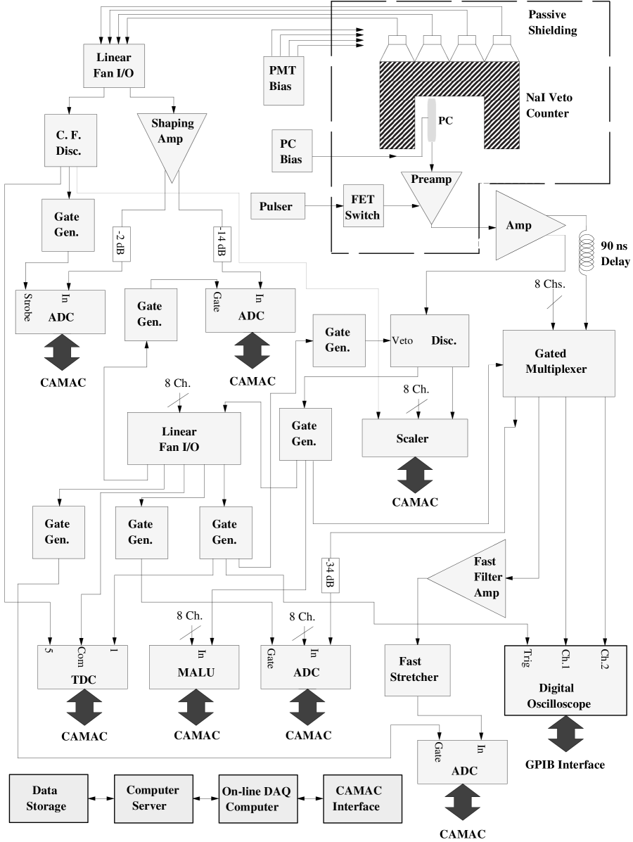
FIG. 4.: Block diagram of one channel of the eight-channel system 3 counting electronics. Abbreviations: PC, proportional counter; DAQ, data acquisition.

To minimize the length of the signal cables, the rack of counting electronics is immediately adjacent to the outer passive shield. The electronics is in a single rack designed to reduce rf interference. The block diagram of a single channel of system 3 is illustrated in Fig. 4. Briefly, the analog signal processing proceeds as follows: the proportional counter anode is directly connected to a charge-sensitive preamplifier. After further amplification the signal is split, with one channel going to the digital logic to determine that an event from that counter has occurred, and a second channel going to a 90 ns cable delay and then to a gated multiplexer. The signals from all 8 counters are input to separate gates of this multiplexer and the appropriate gate is opened by the digital logic for whichever counter has seen an event. The multiplexed output is split into four channels: two go to a digital oscilloscope which records the counter wave form with 8-bit resolution for 800 ns after pulse onset at two different amplification ranges, one appropriate for the ⁷¹Ge $L$ peak and the other appropriate for the $K$ peak. One of the other two signals goes to an integrating ADC to measure the total pulse energy; the second signal is differentiated with a time constant of 10 ns, stretched, and input to a peak-sensing ADC. This second ADC measures the amplitude of the differentiated pulse, called “ADP.” Acquisition can be run in calibration or event acquisition modes. For each event in acquisition mode, the energy, ADP value, time of event, NaI time and energy, and the two digitized wave forms (high- and low-gain channels) are written to disk.

V Selection of Candidate ⁷¹Ge Events

The counting data consist of a set of events for each of which there is a set of measured parameters, such as wave form, energy, NaI coincidence, etc. The first step of analysis is to sort through these events and apply various selection criteria to choose those events that may be from ⁷¹Ge. We will describe here the selection procedure for events measured in counting system 3; the procedure for system 6 is identical except there are no measured wave forms, so the energy is measured by an ADC and the ADP method is used for rise time determination.

A Standard analysis description

The various steps to select potential ⁷¹Ge events are the following:

(1) The first step of event selection is to examine the event wave form and identify two specific types of events: those that saturate the wave form recorder and those that originate from high-voltage breakdown. Saturated events are mostly produced by alpha particles from natural radioactivity in the counter construction materials or from the decay of ²²²Rn that has entered the counter during filling. Such events are easily identified and labeled by looking at the pulse amplitude at the end of the wave form. Saturated pulses have amplitude greater than 16 keV and occur in an average run at a rate of approximately 0.5/day. Since most such pulses are seen after any initial ²²²Rn has decayed, they are mainly from internal counter radioactivity. Events from high-voltage breakdown have a characteristic wave form which rises very steeply and then plateaus. A true pulse from ⁷¹Ge decay, in contrast, rises more slowly and after this initial rise, has a slow, but steady, increase in amplitude as the positive ions are collected. Breakdown pulses are identified by determining the slope of the wave form between 500 and 1000 ns after pulse digitization begins.

(2) To minimize the concentration of Rn, the air in the vicinity of the counters is continuously purged with evaporating liquid nitrogen. Counter calibrations, however, are done with the counter exposed to counting room air which contains an average of 2 pCi of Rn per liter. When the shield is closed and counting begins, a small fraction of the decays of the daughters of ²²²Rn can make pulses inside the counter that mimic those of ⁷¹Ge. To remove these false ⁷¹Ge events, we delete 2.6 h of counting time after any opening of the passive shield, and estimate the background removal efficiency of this time cut to be nearly 100%. See Sec. VII D 2 for further details.

(3) It is possible that the Xe-GeH₄ counter filling may have a small admixture of ²²²Rn that enters the counter when it is filled. Most of the decays of Rn give slow pulses at an energy outside the ⁷¹Ge peaks, but approximately 8% of the pulses from Rn and its daughters make fast pulses in the $K$ peak that are indistinguishable from those of ⁷¹Ge. Since Rn has a half-life of only 3.8 days, these events will occur early in the counting and be falsely interpreted as ⁷¹Ge events. Each ²²²Rn decay is, however, accompanied by three $\alpha$ particles, which are detected with high efficiency and usually produce a saturated pulse in the counter. Since the radon decay chain takes on average only about 1 h from the initiating decay of ²²²Rn to reach ²¹⁰Pb with a 22-yr half-life, deleting all data for a few hours around each saturated event removes most of these false ⁷¹Ge events. We choose to delete from 15 min prior to 3 h after each saturated pulse. The efficiency of this cut in time is 95%. Further details are given in Sec. VII D 1.

(4) All events whose pulse is coincident with a NaI detector response are then eliminated. Since ⁷¹Ge has no $\gamma$ rays associated with its decay, this veto reduces background from natural radioactivity.

TABLE VIII.: Effect of cuts on the experimental live time and events for all runs of SAGE II and SAGE III that were counted in both $L$ and $K$ peaks (except May 1996). The results of the cut on each row include the effect of all cuts on preceding rows. Because the rise time cut varies with energy, no entry can be given for the “2-15 keV” column.

	Live	Number of events
	time	2–15	$L$	$K$
Cut description	(days)	keV	peak	peak
None	4129	4209	1990	821
Shield open time cut	4040	3962	1864	785
Saturated event time cut	3862	3641	1733	728
NaI coincidence cut	3862	1275	1106	519
Rise time cut	3862	NA	408	314

(5) The next step is to set the energy windows for the Ge $L$ and $K$ peaks. The measure of energy is the integral of the pulse wave form for 800 ns after pulse onset. The peak position for each window is based on the calibration with ⁵⁵Fe, with appropriate corrections for polymerization, as described in Sec. IV D, and for nonlinearity, as described in Sec. IV E. If the peak position changes from one calibration to the next, then the energy window for event selection is slid linearly in time between the two calibrations. The resolution at each peak is held constant and is set to be the average of the resolutions with ⁵⁵Fe for all counter calibrations, scaled to the $L$- or $K$-peak energy as described in Sec. IV D. (In the rare cases that the resolution of the first ⁵⁵Fe calibration is larger than the average, the resolution of the first calibration is used throughout the counting.) Events are then accepted as candidates only if their energy is within $\pm 1$ FWHM of the central peak energy.

(6) Finally, events are eliminated unless their rise time is in the range of what is expected for ⁷¹Ge decays. For runs with wave form recording, the rise time is derived from a fit to the pulse shape with an analytical function, as described below in Sec. V B. For those runs without wave form recording, the $L$ peak is not analyzed and the ADP measure of rise time is used to set the acceptance window for $K$-peak events.

For the 30 runs of SAGE II and III that could be counted in both the $L$ and $K$ peaks, the effect on the live time of each successive cut and the total number of candidate ⁷¹Ge events that survive is given in Table VIII. (The run of May 1996 is excluded because the counter was slightly contaminated with residual ³⁷Ar which had been used to measure this counter’s efficiency.) Figure 5 shows all events from these same runs that survive the first four cuts. Events that occurred early in the counting are shown in the upper panel and at the end of counting in the lower panel.

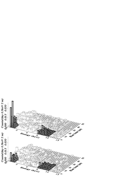
FIG. 5.: Upper panel shows the energy rise time histogram of all events observed during the first 30 days after extraction for all runs that could be counted in both $L$ and $K$ peaks (except May 1996). The live time is 711.1 days. The expected location of the ⁷¹Ge $L$ and $K$ peaks as predicted by the ⁵⁵Fe and ¹⁰⁹Cd calibrations is shown darkened. Lower panel shows the same histogram for all events that occurred during an equal live time interval at the end of counting.

Several runs were compromised and some were completely lost due to operational failures. Failure of an electronic component made it impossible to use the $L$ peak in the extractions of April 1993, May 1993, July 1993, and October 1994. Similar problems made it impossible to make a rise time cut in the $K$ peak for the runs of June 1991, July 1993, October 1994, and October 1997. These runs thus have a larger than normal number of events. If an electronic component fails that deteriorates the rise time response and the failure occurs early in the counting, while the ⁷¹Ge is decaying, our policy is to not use any rise time cut in the $K$ peak and to reject this run in the $L$ peak. If the failure occurs later, the rise time cut is retained and the interval of failure is removed from the data. Extractions in March 1993, January 1995, May 1995, and March 1996 were entirely lost due to counter failure. The extractions of September 1993, September 1994-2, and July 1996 were lost because either the counter stopcock failed or some other gas fill difficulty occurred. Electronic failures caused the loss of the extractions of September 1993-1, May 1994-2, and April 1995. Extractions in June 1995 were lost due to radioactive contamination of the counters with isotopes that were being used at this time for counter efficiency measurement. Finally, we exclude several extractions from one reactor that were systematic studies in preparation for the Cr source experiment. Since their mass was no more than 7.5 tons of gallium, less than one atom of ⁷¹Ge is detected on the average in such runs in the combination of both the $L$ and $K$ peaks. Two-reactor extractions, however, whose mass is approximately 15 tons, give on the average 1.5 ⁷¹Ge events, sufficient to determine the solar neutrino capture rate, albeit with a large error [36].

B Rise time analysis techniques

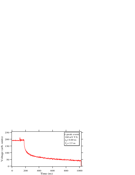
FIG. 6.: ⁷¹Ge events in $L$ and $K$ peaks.

As described in Secs. II B and IV F, the data acquisition system electronics has evolved over the course of SAGE. The data from SAGE I relied entirely on a hardware measurement of the rise time. This ADP technique suffices well in studies of the $K$-peak counter response, but is not capable of adequately differentiating rare $L$-peak events from noise.

Wherever possible for SAGE II, and throughout SAGE III, we derive a parameter that characterizes the rise time from the wave form, and are thus able to present both $L$- and $K$-peak results. For those runs with only ADP data, the $L$ peak cannot be analyzed and we present only $K$-peak data. All wave form data come from counting system 3.

1 Waveform rise time determination – $T_{N}$

Figure 6 shows typical pulses in the $L$ and $K$ peaks from a ⁷¹Ge-filled counter as captured by the digitizing oscilloscope in system 3. There are 256 channels full scale on the y axis corresponding to 1.040 V (130 mV/div) for digitizer channel 1 and 0.160 V (20 mV/div) for channel 2. The x axis has 1024 digitization points each with 1 ns duration. The relevant features of the pulses are the base line from $t=0$ to roughly 120 ns, the dc offset that occurs when the gate opens at 120 ns, and the fast onset of the pulse at about 180 ns. The exact values of these times and offsets vary depending on the counting channel and the run; they even vary slightly from pulse to pulse within a given run. When determining the energy and rise time of the pulse, it is therefore necessary to determine accurately the onset of the pulse both in time and dc voltage level.

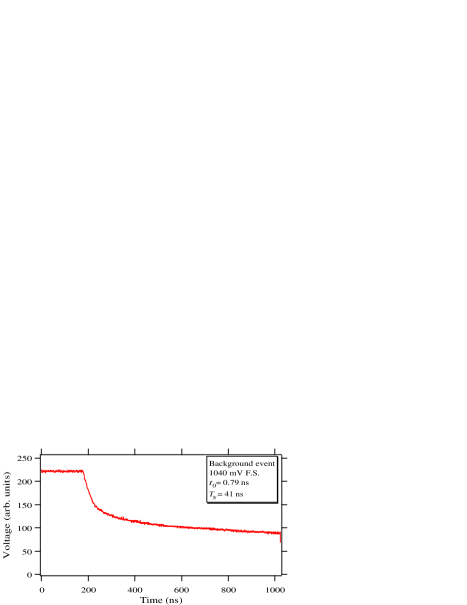
FIG. 7.: Background candidate event in $K$ peak. Note the much slower fall when the pulse begins at $\sim 200$ ns than for the true ⁷¹Ge $K$-peak event in Fig. 6.

By treating the trail of ionization in the proportional counter as a collection of point ionizations and integrating over their arrival time at the anode, it can be shown [37] that the voltage output $V$ of an infinite bandwidth preamplifier as a function of time $t$ after pulse onset has the form

$$\begin{array}[]{rcll}V(0<t<T_{N})&=&V_{0}[&\frac{t+t_{0}}{T_{N}}\ln(1+\frac{t}{t_{0}})-\frac{t}{T_{N}}],\\ V(t>T_{N})&=&V_{0}[&\ln(1+\frac{t-T_{N}}{t_{0}})-1\\ &&&-\frac{t+t_{0}}{T_{N}}\ln(1-\frac{T_{N}}{t+t_{0}})],\end{array}$$ (8)

with $V(t<0)=0$, where $T_{N}$ is the time duration over which the ionization arrives at the anode, $t_{0}$ is a time inversely proportional to the ion mobility, and $V_{0}$ is proportional to the total amount of ionization deposited in the counter. The parameter $T_{N}$ characterizes the rise time of the wave form. For the case of true point ionization, $T_{N}$ should be near zero. When $T_{N}$ is zero, the function reduces to the Wilkinson form $V(t:T_{N}=0)=V_{0}\ln(1+t/t_{0})$. When $T_{N}$ is large, the event is characteristic of extended ionization, and is most likely a background event from a high-energy $\beta$ particle traversing the counter. Figure 7 is an example of such a slow pulse in the $K$ peak.

Because this form for the pulse shape has a sound physical basis and reasonable mathematical simplicity, we fit every pulse that is not identified as saturation or breakdown to Eq. (8). To account for the fact that the pulse onset time $t_{\text{onset}}$ is not at time zero, we replace $t$ by $t-t_{\text{onset}}$, and since the pulse begins at a finite voltage $V_{\text{offset}}$, we replace $V$ by $V-V_{\text{offset}}$. The fit is made from 40 ns before the time of pulse onset to 400 ns after onset. Five parameters are determined by the fit: $t_{\text{onset}}$, $V_{\text{offset}}$, $V_{0}$ (a measure of the energy deposited during the event which is not used in analysis), $t_{0}$ (whose value of slightly less than 1 ns is approximately constant for all pulses), and $T_{N}$ (the rise time).

2 Alternative wave form analysis methods

Although we use fits to $T_{N}$ as our standard analysis technique, we also developed two alternative methods to discriminate pointlike ionization from extended-track ionization in the proportional counter pulses. These serve as checks on the event selection based on $T_{N}$. One technique is based on a fast Fourier transform (FFT) of the digitized wave form. No specific functional form for the pulse is assumed and hence this method has the advantage that it is sensitive to potential alterations in the pulse shape. See Appendix B for further information concerning the FFT method. The second method of wave form analysis that was investigated also assumes no particular form for the pulse. This method, called the “RST method,” deconvolutes the observed wave form to find the initial ionization pattern in the counter. See Appendix C for further details.

Since these three techniques are sensitive to different characteristics of the wave form, their selection of events is, not unexpectedly, different. Nonetheless, when many data sets are considered in combination, their results for the overall production rate are in good agreement, which provides strong support for the validity of our wave form analysis procedure.

3 Hardware rise rime measurement: ADP

The amplitude of the differentiated pulse is proportional to the product of the original pulse amplitude and the inverse rise time. The quantity ADP/energy is thus proportional to the inverse rise time. Events due to low-energy Auger electrons and x rays that produce point ionization in the counter all have a fast rise time. Events with a slower rise time (small ADP) are due to background pulses that produce extended ionization. Events with a very fast rise time (large ADP) are due to electronic noise or high-voltage breakdown.

Inherent in an ADP analysis is the uncertainty that arises from an imprecise knowledge of the offset for a given run. Nonzero offset occurs when the gate is opened after an event trigger. The electronic components which process the pulse are subject to small drifts in their offsets that are functions of external parameters, such as temperature. These nonzero offsets contribute to the dc offset on which the event pulse rides. Our approach has been to extrapolate ADP vs energy plots from the ⁵⁵Fe calibrations using the 5.9-keV peak and the escape peak to obtain an offset for each calibration. Since the offsets are typically distributed in a Gaussian manner with a sigma of 1 or 2 channels, the average is a good approximation when determining the $K$-peak selection window. For the $L$ peak, however, uncertainties of a few channels lead to significant variations in event selection. Utilizing the digitized pulses, it is possible to eliminate this uncertainty by determining every offset on a pulse-by-pulse basis.

A further disadvantage of the ADP method is that it is only responsive to the initial rise of the pulse. Occasional small pulses from high-voltage breakdown have rise time the same as for true $L$-peak ⁷¹Ge pulses, but after their initial rise they turn flat, rather than gently rise as the positive ions are collected as with a real ⁷¹Ge event. A breakdown event of this type is not distinguished from a ⁷¹Ge event by the ADP method, but is easily recognized by examining the recorded wave form long after pulse onset.

C Calibration of rise time response

To determine the values of $T_{N}$ for true ⁷¹Ge pulses, we have filled counters with typical gas mixtures (20% GeH₄ and 80% Xe at a pressure of 620 mm Hg), added a trace of active ⁷¹GeH₄, and measured the pulses in each of the system 3 counting slots. All events inside 2 FWHM of the $L$ and $K$ peaks are then selected and the rise time $T_{N}$ of each event calculated with Eq. (8). The rise time values are arranged in ascending order and an upper rise time limit set such that 5% of the events are excluded. This leads to event selection limits on $T_{N}$ of 0.0–10.0 ns in the $L$ peak and 0.0–18.4 ns in the $K$ peak. The variation with electronics channel and with counter filling, over the range of our usual gas mixtures, was measured to be approximately 1.2 ns. We choose to fix the event selection limits at the values given above, and include in the systematic error an uncertainty in the efficiency of $\pm 1$% due to channel and filling variations. A major advantage of using $T_{N}$ is that the rise time limits are fixed and are the same for all extractions. The purpose of the calibrations with ⁵⁵Fe and other sources is solely to determine the energy scale.

For those runs in which the ADP method of rise time discrimination is used, the limits for the ADP cut are determined separately for each run from the ⁵⁵Fe calibrations. Histograms of the values of ADP/energy for the events within 2 FWHM of the 5.9-keV energy peak are analyzed to determine the cut point for 1% from the fast region (to eliminate noise) and 4% from the slow region (to eliminate background). All calibrations from a run are analyzed and the ADP window for event selection is slid linearly in time from one calibration to the next.

VI Statistical Analysis and Results of Single Runs

In this section we describe how the data are analyzed to determine the ⁷¹Ge production rate. We then give the results for individual runs and for all runs in the $L$- and $K$-peak regions.

A Single-run results

The above selection criteria result in a group of events from each extraction in both the $L$- and $K$-peak regions which are candidate ⁷¹Ge decays. To determine the rate at which ⁷¹Ge was produced during the exposure time, it is assumed in each peak region that these events originate from two sources: the exponential decay of a fixed number of ⁷¹Ge atoms and a constant-rate background (different for each peak). Under this assumption the likelihood function [38] for each peak region is

$${\cal L}=e^{-m}\prod_{i=1}^{N}(b+ae^{-\lambda t_{i}}),$$ (9)

where

$$m = bT+a\Delta/\lambda,$$ (10)

$$T = \sum_{k=1}^{n}(t_{ek}-t_{bk}),$$ (11)

$$\Delta = \sum_{k=1}^{n}(e^{-\lambda t_{bk}}-e^{-\lambda t_{ek}}).$$ (12)

Here $b$ is the background rate, $\lambda$ is the decay constant of ⁷¹Ge, $t_{i}$ is the time of occurrence of each event with $t=0$ at the time of extraction, and $N$ is the total number of candidate events. The production rate $p$ of ⁷¹Ge is related to the parameter $a$ by

$$a=\epsilon p(1-e^{-\lambda\Theta}),$$ (13)

where $\Theta=t_{E}-t_{B}$ is the exposure time (i.e., the time of end of exposure $t_{E}$ minus the time of beginning of exposure $t_{B}$), and $\epsilon$ is the total efficiency for the extraction (i.e., the product of extraction and counting efficiencies). The total counting live time is given by $T$ and is a sum over the $n$ counting intervals, each of which has a starting time $t_{bk}$ and ending time $t_{ek}$. The parameter $\Delta$ is the live time weighted by the exponential decay of ⁷¹Ge. Its value would be unity if counting began at the end of extraction and continued indefinitely. We convert the production rate (in ⁷¹Ge atoms produced per day) to the solar neutrino capture rate (in SNU) using the conversion factor $2.977\times 10^{-4}$ atoms of ⁷¹Ge produced/(SNU day ton of gallium), where the mass of gallium exposed in each extraction is given in Table III.

Because of the eccentricity of the Earth’s orbit, the Earth-Sun distance, and thus the production rate, varies slightly during the year. We correct the production rate for this effect by multiplying $\epsilon$ by the factor $1+C$ where $C$ is given by

$$C=\bigg{(}\frac{2e}{S[1+r^{2}]}\bigg{)}[ \cos X_{E} +r\sin X_{E}$$ (14)

$$-(1-S)( \cos X_{B} +r\sin X_{B})],$$ (15)

with

$$r = \omega/\lambda,$$ (16)

$$X_{E} = \omega(t_{E}-t_{p}),$$ (17)

$$X_{B} = \omega(t_{B}-t_{p}),$$ (18)

$$S = 1-e^{-\lambda\Theta}.$$ (19)

Here $e$ is the eccentricity of the orbit ($e=0.0167$), $\omega$ is the angular frequency ($\omega=2\pi/365.25\text{ day}^{-1}$), and $t_{p}$ is the moment of perihelion passage, which has been 2–5 January for the past number of years. We use $t_{p}=3.5$ days.

The best estimate of the solar neutrino capture rate in each peak region is determined by finding the values of $a$ and $b$ which maximize $\cal L$. In doing so we exclude unphysical regions; i.e., we require $a>0$ and $b>0$. The uncertainty in the capture rate is found by integrating the likelihood function over the background rate to provide a likelihood function of signal only, and then locating the minimum range in signal which includes 68% of the area under that curve. This procedure is done separately for the $L$ and $K$ peaks and the results are given in Tables IX and X. We call the set of events in each peak region a “data set.”

TABLE IX.: Results of analysis of $L$-peak events. $Nw^{2}$ is a measure of the goodness of fit. See [39] for its calculation and use. The probability values are derived from 1000 simulations and have an uncertainty of $\sim 1.5$%. The total counting live time is 10.379 yr. The entries in columns 2–4 include all analysis time cuts.

	$Lead$	$Live$		$Numberof$	$Number$	$Best$	68% conf.
Exposure	$time$	$time$		$candidate$	$fitto$	$fit$	range			$Probability$
date	$(h)$	$(days)$	$Delta$	$events$	${}^{71}Ge$	$(SNU)$	(SNU)		$Nw^{2}$	$(\%)$
Sep. 92	$29.0$	$103.8$	$0.811$	$7.$	$4.0$	$109.$	46–	$174.$	$0.039$	$82.$
Oct. 92	$27.3$	$96.3$	$0.839$	$10.$	$0.0$	$0.$	0–	$61.$	$0.179$	$19.$
Nov. 92	$30.7$	$66.7$	$0.688$	$12.$	$0.0$	$0.$	0–	$62.$	$0.238$	$12.$
Dec. 92	$26.7$	$47.5$	$0.835$	$10.$	$7.4$	$153.$	51–	$208.$	$0.055$	$65.$
Jan. 93	$29.9$	$23.4$	$0.518$	$4.$	$4.0$	$135.$	35–	$181.$	$0.092$	$67.$
June 93	$33.3$	$120.7$	$0.699$	$9.$	$1.1$	$29.$	0–	$107.$	$0.490$	$2.$
Oct. 93-2	$51.9$	$71.6$	$0.686$	$2.$	$2.0$	$193.$	19–	$297.$	$0.097$	$55.$
Oct. 93-3	$31.6$	$102.7$	$0.772$	$3.$	$3.0$	$287.$	88–	$428.$	$0.078$	$68.$
July 94	$45.6$	$136.0$	$0.782$	$10.$	$2.2$	$65.$	11–	$131.$	$0.026$	$95.$
Aug. 94	$32.6$	$116.4$	$0.838$	$20.$	$0.0$	$0.$	0–	$67.$	$0.056$	$73.$
Sep. 94-1	$40.5$	$120.0$	$0.729$	$20.$	$4.7$	$171.$	54–	$300.$	$0.087$	$32.$
Nov. 94	$30.4$	$112.3$	$0.660$	$10.$	$2.7$	$76.$	18–	$143.$	$0.041$	$79.$
July 95	$35.5$	$110.6$	$0.776$	$16.$	$1.2$	$35.$	0–	$104.$	$0.336$	$3.$
Aug. 95	$35.2$	$108.9$	$0.698$	$16.$	$3.9$	$113.$	42–	$200.$	$0.095$	$28.$
Sep. 95	$124.3$	$80.4$	$0.561$	$23.$	$0.2$	$8.$	0–	$179.$	$0.160$	$23.$
Oct. 95	$39.3$	$120.7$	$0.793$	$17.$	$3.2$	$169.$	33–	$319.$	$0.041$	$78.$
Nov. 95	$37.2$	$149.9$	$0.759$	$19.$	$8.4$	$214.$	124–	$310.$	$0.064$	$45.$
Dec. 95-2	$78.3$	$119.9$	$0.530$	$22.$	$0.8$	$40.$	0–	$174.$	$0.102$	$42.$
Jan. 96	$33.9$	$141.2$	$0.767$	$21.$	$0.0$	$0.$	0–	$61.$	$0.065$	$66.$
May 96	$35.2$	$117.8$	$0.628$	$25.$	$3.5$	$104.$	23–	$200.$	$0.038$	$82.$
Aug. 96	$32.9$	$148.7$	$0.790$	$20.$	$5.6$	$126.$	58–	$204.$	$0.048$	$68.$
Oct. 96	$33.6$	$155.5$	$0.785$	$11.$	$0.0$	$0.$	0–	$48.$	$0.119$	$39.$
Nov. 96	$35.0$	$162.5$	$0.795$	$13.$	$0.2$	$5.$	0–	$58.$	$0.042$	$85.$
Jan. 97	$34.5$	$160.0$	$0.816$	$16.$	$1.2$	$24.$	0–	$68.$	$0.581$	$1.$
Mar. 97	$36.3$	$160.9$	$0.814$	$10.$	$2.6$	$45.$	9–	$89.$	$0.126$	$17.$
Apr. 97	$35.0$	$167.4$	$0.791$	$12.$	$0.0$	$0.$	0–	$27.$	$0.108$	$45.$
June 97	$35.8$	$173.4$	$0.797$	$16.$	$4.5$	$95.$	40–	$161.$	$0.089$	$30.$
July 97	$37.0$	$140.0$	$0.752$	$13.$	$0.7$	$14.$	0–	$61.$	$0.238$	$10.$
Sep. 97	$33.6$	$166.6$	$0.826$	$12.$	$1.1$	$24.$	0–	$77.$	$0.059$	$64.$
Oct. 97	$34.2$	$149.5$	$0.780$	$19.$	$4.7$	$99.$	42–	$167.$	$0.041$	$76.$
Dec. 97	$34.4$	$137.1$	$0.726$	$15.$	$3.1$	$69.$	18–	$131.$	$0.045$	$73.$
Combined (31 data sets)				$433.$	$64.3$	$55.$	43–	$68.$	$0.020$	$>99.$

TABLE X.: Results of analysis of $K$-peak events. The uncertainty in the probability is $\sim 1.5$%. No probability can be given for exposure Oct. 93-1 because no counts were detected. The total counting live time is 18.342 yr.

	$Lead$	$Live$		$Numberof$	$Number$	$Best$	68% conf.
Exposure	$time$	$time$		$candidate$	$fitto$	$fit$	range			$Probability$
date	$(hours)$	$(days)$	$Delta$	$events$	${}^{71}Ge$	$(SNU)$	(SNU)		$Nw^{2}$	$(\%)$
Jan. 90	$25.0$	$57.4$	$0.849$	$8.$	$0.0$	$0.$	0–	$64.$	$0.367$	$4.$
Feb. 90	$25.0$	$57.3$	$0.886$	$2.$	$2.0$	$95.$	18–	$159.$	$0.164$	$26.$
Mar. 90	$25.0$	$47.5$	$0.839$	$9.$	$2.8$	$107.$	0–	$224.$	$0.053$	$66.$
Apr. 90	$29.8$	$90.4$	$0.881$	$9.$	$0.0$	$0.$	0–	$112.$	$0.104$	$40.$
July 90	$22.6$	$59.3$	$0.870$	$15.$	$0.0$	$0.$	0–	$213.$	$0.142$	$28.$
June 91	$20.5$	$108.3$	$0.904$	$10.$	$0.4$	$13.$	0–	$119.$	$0.211$	$14.$
July 91	$26.1$	$59.2$	$0.877$	$1.$	$1.0$	$55.$	0–	$115.$	$0.159$	$26.$
Aug. 91	$73.8$	$94.4$	$0.651$	$16.$	$9.8$	$412.$	243–	$577.$	$0.036$	$83.$
Sep. 91	$35.3$	$68.9$	$0.827$	$8.$	$3.5$	$73.$	20–	$126.$	$0.041$	$79.$
Nov. 91	$40.8$	$112.6$	$0.822$	$14.$	$2.4$	$48.$	0–	$102.$	$0.095$	$30.$
Dec. 91	$26.2$	$111.8$	$0.917$	$10.$	$10.0$	$180.$	99–	$217.$	$0.063$	$77.$
Feb. 92-1	$21.5$	$192.7$	$0.900$	$14.$	$0.0$	$0.$	0–	$43.$	$0.057$	$74.$
Feb. 92-2	$43.0$	$43.2$	$0.800$	$1.$	$1.0$	$101.$	0–	$192.$	$0.085$	$88.$
Mar. 92	$26.0$	$167.8$	$0.840$	$21.$	$10.1$	$245.$	155–	$342.$	$0.043$	$72.$
Apr. 92	$21.5$	$144.9$	$0.717$	$15.$	$2.3$	$55.$	13–	$111.$	$0.143$	$18.$
May 92	$54.0$	$114.9$	$0.843$	$4.$	$0.0$	$0.$	0–	$74.$	$0.134$	$30.$
Sep. 92	$29.0$	$103.8$	$0.811$	$6.$	$2.1$	$55.$	12–	$104.$	$0.108$	$25.$
Oct. 92	$27.3$	$134.2$	$0.840$	$11.$	$2.7$	$52.$	13–	$98.$	$0.046$	$71.$
Nov. 92	$30.7$	$123.4$	$0.695$	$16.$	$5.1$	$130.$	57–	$210.$	$0.046$	$68.$
Dec. 92	$26.7$	$140.7$	$0.871$	$18.$	$9.1$	$176.$	107–	$250.$	$0.075$	$36.$
Jan. 93	$29.9$	$119.1$	$0.816$	$13.$	$5.6$	$111.$	45–	$181.$	$0.130$	$14.$
Feb. 93	$26.2$	$169.6$	$0.839$	$3.$	$0.0$	$0.$	0–	$48.$	$0.116$	$41.$
Apr. 93	$25.0$	$155.3$	$0.820$	$7.$	$2.9$	$71.$	25–	$124.$	$0.041$	$82.$
May 93	$33.4$	$126.8$	$0.411$	$8.$	$1.4$	$64.$	5–	$153.$	$0.073$	$51.$
June 93	$33.3$	$120.7$	$0.699$	$9.$	$2.1$	$51.$	3–	$111.$	$0.154$	$11.$
July 93	$27.5$	$124.5$	$0.761$	$28.$	$7.6$	$224.$	114–	$348.$	$0.040$	$78.$
Aug. 93-1	$26.8$	$129.0$	$0.877$	$4.$	$2.5$	$66.$	20–	$116.$	$0.048$	$79.$
Aug. 93-2	$53.8$	$53.0$	$0.769$	$1.$	$1.0$	$120.$	0–	$227.$	$0.093$	$67.$
Oct. 93-1	$26.7$	$54.5$	$0.733$	$0.$	$0.0$	$0.$	0–	$158.$	NA	NA
Oct. 93-2	$51.9$	$72.6$	$0.694$	$2.$	$0.8$	$69.$	0–	$198.$	$0.048$	$86.$
Oct. 93-3	$31.6$	$103.7$	$0.782$	$4.$	$0.3$	$27.$	0–	$192.$	$0.024$	$99.$
July 94	$45.6$	$136.7$	$0.783$	$12.$	$1.1$	$30.$	0–	$88.$	$0.056$	$68.$
Aug. 94	$32.6$	$117.2$	$0.841$	$7.$	$3.0$	$71.$	25–	$123.$	$0.042$	$78.$
Sep. 94-1	$40.5$	$120.8$	$0.751$	$10.$	$2.6$	$87.$	22–	$165.$	$0.043$	$76.$
Oct. 94	$55.4$	$120.3$	$0.681$	$44.$	$4.8$	$136.$	27–	$257.$	$0.075$	$45.$
Nov. 94	$30.4$	$112.3$	$0.660$	$13.$	$5.6$	$164.$	79–	$259.$	$0.035$	$84.$
Dec. 94	$29.3$	$100.0$	$0.803$	$9.$	$0.0$	$0.$	0–	$236.$	$0.184$	$19.$
Mar. 95	$29.3$	$151.4$	$0.772$	$23.$	$3.7$	$147.$	47–	$266.$	$0.042$	$77.$
July 95	$35.5$	$110.6$	$0.776$	$17.$	$4.3$	$128.$	39–	$229.$	$0.114$	$19.$
Aug. 95	$35.2$	$108.9$	$0.698$	$8.$	$3.6$	$100.$	38–	$168.$	$0.058$	$59.$
Sep. 95	$124.3$	$80.4$	$0.561$	$10.$	$1.0$	$48.$	0–	$201.$	$0.144$	$19.$
Oct. 95	$39.3$	$120.7$	$0.793$	$9.$	$3.3$	$160.$	51–	$286.$	$0.060$	$54.$
Nov. 95	$37.2$	$149.9$	$0.759$	$13.$	$2.7$	$66.$	18–	$125.$	$0.039$	$83.$
Dec. 95-2	$78.3$	$119.9$	$0.530$	$18.$	$0.0$	$0.$	0–	$127.$	$0.044$	$85.$
Jan. 96	$33.9$	$141.2$	$0.767$	$14.$	$4.6$	$117.$	45–	$193.$	$0.091$	$29.$
May 96	$35.2$	$117.8$	$0.628$	$6.$	$2.3$	$66.$	13–	$126.$	$0.028$	$95.$
Aug. 96	$32.9$	$148.9$	$0.800$	$6.$	$0.0$	$0.$	0–	$51.$	$0.102$	$45.$
Oct. 96	$33.6$	$155.5$	$0.785$	$10.$	$5.0$	$107.$	55–	$165.$	$0.066$	$47.$
Nov. 96	$35.0$	$162.5$	$0.795$	$15.$	$1.9$	$40.$	0–	$88.$	$0.110$	$29.$
Jan. 97	$34.5$	$160.0$	$0.816$	$8.$	$1.4$	$29.$	0–	$70.$	$0.123$	$23.$
Mar. 97	$36.3$	$160.9$	$0.814$	$14.$	$3.6$	$64.$	20–	$116.$	$0.058$	$52.$
Apr. 97	$35.0$	$167.4$	$0.791$	$10.$	$4.2$	$84.$	38–	$137.$	$0.052$	$63.$
June 97	$35.8$	$160.2$	$0.797$	$11.$	$5.8$	$121.$	65–	$183.$	$0.033$	$86.$
July 97	$37.0$	$127.3$	$0.751$	$9.$	$0.0$	$0.$	0–	$37.$	$0.204$	$16.$
Sep. 97	$33.6$	$124.5$	$0.794$	$5.$	$2.6$	$61.$	22–	$107.$	$0.109$	$29.$
Oct. 97	$34.2$	$149.5$	$0.780$	$7.$	$0.3$	$6.$	0–	$42.$	$0.429$	$3.$
Dec. 97	$34.4$	$108.4$	$0.519$	$9.$	$3.0$	$90.$	31–	$159.$	$0.044$	$77.$
Combined (57 data sets)				$604.$	$143.7$	$73.$	64–	$82.$	$0.110$	$25.$

TABLE XI.: Results of combined analysis of $L$-peak and $K$-peak events for all 31 runs that could be analyzed in both peaks. The uncertainty in the probability is $\sim 1.5$%. Treating the $L$- and $K$-peak regions as two separate data sets, the total counting live time is 21.282 yr.

	$Numberof$	$Number$	$Best$	68% conf.
Exposure	$candidate$	$fitto$	$fit$	range			Prob.
date	$events$	${}^{71}Ge$	$(SNU)$	(SNU)		$Nw^{2}$	(%)
Sep. 92	$13.$	$6.0$	$79.$	44–	$123.$	0.097	$25.$
Oct. 92	$21.$	$3.3$	$32.$	4–	$67.$	0.105	$26.$
Nov. 92	$28.$	$4.3$	$56.$	10–	$111.$	0.047	$70.$
Dec. 92	$28.$	$16.8$	$168.$	115–	$229.$	0.057	$53.$
Jan. 93	$17.$	$10.0$	$124.$	81–	$177.$	0.089	$32.$
June 93	$18.$	$3.3$	$42.$	4–	$92.$	0.557	$<1.$
Oct. 93-2	$4.$	$3.0$	$141.$	60–	$245.$	0.049	$83.$
Oct. 93-3	$7.$	$4.0$	$185.$	80–	$303.$	0.052	$77.$
July 94	$22.$	$3.4$	$47.$	9–	$94.$	0.027	$95.$
Aug. 94	$27.$	$3.9$	$46.$	15–	$85.$	0.075	$52.$
Sep. 94-1	$30.$	$6.5$	$112.$	50–	$188.$	0.082	$39.$
Nov. 94	$23.$	$8.0$	$116.$	66–	$176.$	0.015	$>99.$
July 95	$33.$	$5.0$	$74.$	19–	$138.$	0.063	$55.$
Aug. 95	$24.$	$7.4$	$105.$	60–	$161.$	0.061	$56.$
Sep. 95	$33.$	$1.2$	$28.$	0–	$142.$	0.058	$73.$
Oct. 95	$26.$	$6.5$	$163.$	75–	$270.$	0.019	$>99.$
Nov. 95	$32.$	$10.2$	$127.$	78–	$185.$	0.032	$88.$
Dec. 95-2	$40.$	$0.5$	$12.$	0–	$95.$	0.068	$62.$
Jan. 96	$35.$	$3.5$	$45.$	0–	$101.$	0.047	$76.$
May 96	$31.$	$5.3$	$78.$	31–	$136.$	0.039	$90.$
Aug. 96	$26.$	$4.5$	$51.$	14–	$96.$	0.089	$35.$
Oct. 96	$21.$	$5.4$	$58.$	28–	$95.$	0.046	$74.$
Nov. 96	$28.$	$1.9$	$21.$	0–	$57.$	0.103	$37.$
Jan. 97	$24.$	$2.6$	$26.$	0–	$60.$	0.190	$13.$
Mar. 97	$24.$	$6.1$	$54.$	24–	$90.$	0.134	$15.$
Apr. 97	$22.$	$2.7$	$27.$	3–	$57.$	0.037	$86.$
June 97	$27.$	$10.4$	$109.$	71–	$155.$	0.078	$35.$
July 97	$22.$	$0.0$	$0.$	0–	$24.$	0.333	$7.$
Sep. 97	$17.$	$4.3$	$49.$	22–	$84.$	0.043	$80.$
Oct. 97	$26.$	$3.4$	$36.$	9–	$72.$	0.083	$49.$
Dec. 97	$24.$	$6.2$	$80.$	40–	$128.$	0.031	$89.$
Combined	$753.$	$152.1$	$64.$	56–	$72.$	0.033	$93.$

The overall likelihood function for a single extraction is the product of the separate likelihood functions for the $L$- and $K$-peak regions. The best fit capture rate is found by maximizing this function, allowing the independent background rates in the $L$ and $K$ peaks to be free variables. The uncertainty in this result is determined by finding the values of the capture rate at which the logarithm of the likelihood function decreases by 0.5, again choosing the background rates at these two points to be those which maximize the likelihood function. The results for all extractions that could be analyzed in both peaks are given in Table XI.

The capture rate for each extraction of all runs of SAGE is plotted in Fig. 8. These results are derived from the $K$ peak plus $L$ peak wherever possible, otherwise from the $K$ peak alone. For those readers who may be interested in looking for temporal phenomena, the beginning time $t_{B}$ and ending time $t_{E}$ for each run can be inferred from the mean exposure date $t_{m}$ and total exposure time $\Theta$ given in Table III by the relationships

$$t_{B} = t_{m}-\frac{1}{\lambda}\ln\bigg{(}\frac{1+e^{\lambda\Theta}}{2}\bigg{)},$$ (20)

$$t_{E} = \Theta-t_{B}.$$ (21)

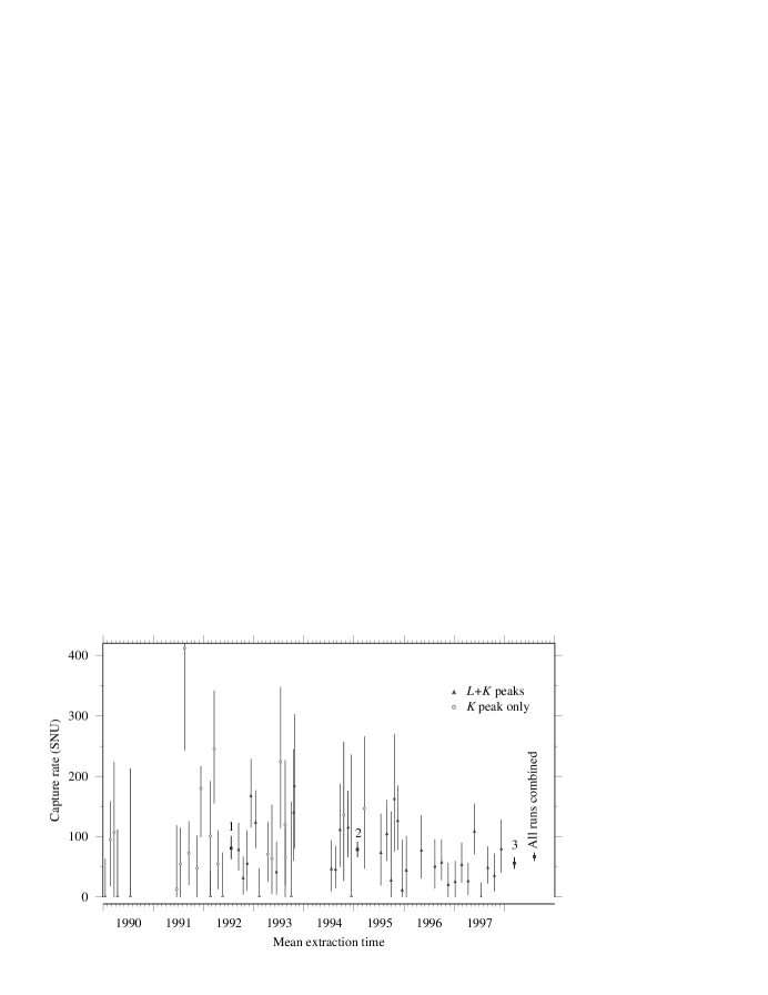
FIG. 8.: Capture rate for each extraction as a function of time. All uncertainties are only statistical. The symbols 1, 2, and 3 show the combined result for SAGE I, II, and III, respectively.

B Global fits

The combined likelihood function for any set of extractions is the product of the overall likelihood functions for each extraction. The best fit capture rate for the set of extractions is determined by maximizing this function, requiring the production rate per unit mass of Ga to be the same for each extraction, and allowing the background rates in both the $L$ and $K$ peaks to be different for each extraction. The uncertainty is found in the same way as for the $L$- and $K$-peak combination for a single extraction. There are a number of other techniques for estimating the uncertainties in addition to the two described and used here. When many runs are combined, the likelihood as a function of capture rate approaches a Gaussian, and the difference between the results of these techniques becomes slight.

The results of global fits to our data are given in Sec. VIII.

VII Systematic Uncertainties

There are four basic sources of systematic error in SAGE: uncertainty in the chemical extraction efficiency, uncertainty in the counting efficiency, uncertainty due to nonsolar neutrino production of ⁷¹Ge (such as by cosmic rays), and uncertainty due to nonconstant events which mimic ⁷¹Ge (such as may be made by ²²²Rn). Table XII summarizes the results of our consideration of all these effects and additional information regarding each of these items follows.

TABLE XII.: Summary of the systematic uncertainties. The SNU values for extraction and counting efficiency are based on a rate of 67.2 SNU.

	Uncertainty
Origin of uncertainty	$inpercent$	$inSNU$
Extraction efficiency
Ge carrier mass	$\pm 2.1\%$	$\pm 1.4$
Mass of extracted Ge	$\pm 2.5\%$	$\pm 1.7$
Residual Ge carrier	$\pm 0.8\%$	$\pm 0.5$
Ga mass	$\pm 0.3\%$	$\pm 0.2$
Total (extraction)	$\pm 3.4\%$	$\pm 2.3$
Counting efficiency
Volume efficiency	$\pm 1.4\%$	$\pm 0.9$
End losses	$\pm 0.5\%$	$\pm 0.3$
Monte Carlo interpolation	$\pm 1.0\%$	$\pm 0.7$
Shifts of gain	$-3.1\%$	$+2.1$
Resolution	$+0.5\%,-0.7\%$	$-0.3,+0.5$
Rise time limits	$\pm 1.0\%$	$\pm 0.7$
Lead and exposure times	$\pm 0.8\%$	$\pm 0.5$
Total (counting)	$+2.3\%,-3.9\%$	$-1.5,+2.6$
Nonsolar neutrino production of 71Ge
Fast neutrons		$<-0.02$
232Th		$<-0.04$
226Ra		$<-0.7$
Cosmic-ray muons		$<-0.7$
Total (nonsolar)		$<-1.0$
Background events that mimic 71Ge
Internal 222Rn		$<-0.2$
External 222Rn		$0.0$
Internal 69Ge		$<-0.6$
Total (background events)		$<-0.6$
Total		$-3.0,+3.5$

A Chemical extraction efficiency

The way in which the chemical extraction efficiency is determined was described in Sec. III B. There are four sources of uncertainty.

1 Mass of Ge carrier

The extraction efficiency is measured by adding to the Ga metal several slugs of Ga-Ge alloy which contain a known mass of Ge. This alloy is produced in large batches by reduction of Ge by Ga metal from chloride solution, and then divided into several hundred small slugs, each of which weighs 18–20 g and contains about 40 $\mu$g of Ge. The equality of Ge content was measured by extracting the Ge from a few dozen slugs. The standard deviation of these measurements was 2.1%, which we take as the uncertainty in the mass of added Ge carrier.

2 Mass of extracted Ge

There is also an uncertainty in how much carrier has been synthesized into GeH₄. This is determined by the accuracy to which the GeH₄ volume can be determined and is estimated to be 2.5%.

3 Residual Ge carrier

Since the extraction of carrier Ge is not complete, residual Ge carrier from preceding extractions will contribute to the extraction efficiency measurement. Each extraction for solar neutrino data is followed by a second extraction to remove this surplus carrier. The amount removed during the first two extractions is at least 95%, but is uncertain as described above, which leads to an uncertainty in the amount of remaining carrier. The extraction efficiency uncertainty due to the uncertainty in the residual carrier is $\pm 0.8$%.

4 Mass of Ga

The total mass of Ga has been weighed periodically with a precision of 0.3%. The amount removed during each extraction is small (typically 0.1%) and is known well (2%). We take the uncertainty in the Ga mass for all runs to be $\pm 0.3$%.

B Counting efficiency

The counter efficiency is calculated using Eq. 5. There are thus three sources of uncertainty: the volume efficiency $\epsilon_{v}$, the end effects (or equivalently the fraction of degraded events), and the gas efficiency.

1 Volume efficiency

As described in Sec. IV C, the volume efficiency of seven counters of the “LA” type has been directly measured with an uncertainty of 0.6%. These seven counters were used for 48 of our 88 data sets. The uncertainty in $\epsilon_{v}$ for counters of this same type used in 36 other data sets is estimated from the spread in the measured $\epsilon_{v}$ for the measured counters, which is $\pm 2.3$% relative uncertainty. The uncertainty in $\epsilon_{v}$ for counters of the “Ni” and “RD” types, which were used for four data sets, is taken as $\pm 3$%. Averaging over the different types of counters used for all extractions, the uncertainty assigned to volume efficiency is taken as $\pm 1.4$%.

2 End effects

The reduced electric field near the ends of the counter cathode results in a fraction of events that lie outside the $\pm 1$ FWHM energy windows. Uncertainties in these end effects are due to variations in the physical dimensions of the counters. Based on measurements of various “LA” counters, these dimensional differences lead to an uncertainty of $\pm 4.1$% in the end effect. This gives $\pm 0.5$% relative uncertainty in the factor $(1-f_{D})$. This should be valid for measurements made with the “LA” counters, which were used for most of our data, and this value is taken for the entire data set.

3 Monte Carlo interpolation of measured gas parameters

The uncertainties in the gas efficiency consist of three components: uncertainty in the Monte Carlo calculations, uncertainty in the measured gas pressure, and uncertainty in the measured percentage of GeH₄. The limited statistics used in the Monte Carlo calculations to determine the constants in the gas efficiency formula leads to an uncertainty of 1.0% in the determination of the gas efficiency. The uncertainty in the gas pressure measurements is $\pm 5$ Torr, which corresponds to an uncertainty in the gas efficiency for a typical counter filling (710 Torr at 24% GeH₄) of $\pm 0.2$% relative change. The uncertainty in the measured percentage of GeH₄ is taken to be $\pm 1$%, which corresponds to an uncertainty in the gas efficiency for an average counter filling of $\pm 0.2$% relative change. Adding these three contributions in quadrature yields a relative total uncertainty in the gas efficiency of $\pm 1.0$%.

4 Gain shifts

If the calibration mean shifts between two calibrations, there is an error made in the efficiency estimate. This error has been minimized by two features of our standard analysis. First, we use a two FWHM wide energy window. Since the peak is relatively Gaussian and the window limits are far out on the tail, uncertainties in the location of the centroid of the peak do not greatly affect the efficiency. Second, by sliding the energy window between calibrations we hope to minimize any error in estimating the centroid due to the observed gain shifts. Although the correction for nonlinearity of the counter response [Eq. (6)] results in an additional uncertainty in the gain of 0.7%, the total uncertainty in the gain is dominated by the shifts.

To estimate the error generated by using an incorrect centroid, we computed the area under a Gaussian between two integration limits which are shifted by an amount $\delta$. We then compared this number to the 0.9815 number expected from integration limits of $\pm 2$ FWHM. Using a typical $K$-peak resolution of 20%–23% we calculated the true efficiency for various values of $\delta$ expressed as a fraction of the true mean.

Typical gain shifts are of the order of a few percent. This results in an uncertainty of approximately $-3.1$% in the efficiency. Note that this effect can only decrease our efficiency so it is a one sided systematic uncertainty.

5 Energy resolution

As a result of the statistics of our calibration spectra, the resolution is known to about 2.1%. For the $K$ peak, there is an additional uncertainty due to the counter nonlinearity [Eq. (7)] of $\pm 4.5$%. Adding these in quadrature, the uncertainty in the resolution results in an uncertainty in the efficiency of about +0.5%, $-0.7$%. Again, because the energy window is so wide, the uncertainty in the efficiency due to the resolution uncertainty is not large.

6 Rise time limits

As described in Section V C, when the wave form method of rise time determination is used, there is an uncertainty in the efficiency of $\pm 1$% that arises from changes in the rise time limits due to counting channel and filling variations. For those runs that used the ADP method of rise time determination, we can find the uncertainty of the ADP cut as follows: Usually a calibration has between 1000 and 5000 events in the peak. We base our lower ADP threshold on 4% of those or 40–200 events. This small number of events is subject to statistical fluctuations. For the most extreme case, we take the square root of 40 (6.4) and notice that the efficiency due to the ADP cut could actually be between 94.4% and 95.6% instead of the 95% we believe it to be. Thus this is a $\pm 0.6$% uncertainty. Since the vast majority of our data are based on wave form analysis, we use $\pm 1$% for all runs.

7 Lead and exposure times

Because extraction usually occurs from several reactors over the course of 6–10 h, there is an uncertainty in the exposure time and in the time from extraction to the start of counting (which we call the “lead time”) of roughly 3 h. The lead time is typically 36 h and the exposure time is typically 34 days. These small uncertainties make a small contribution to the uncertainty associated with the solar neutrino flux. By Eq. (13), the solar neutrino production rate $p$ is proportional to the quantity $[e^{-\lambda t_{\text{lead}}}(1-e^{-\lambda\Theta})]^{-1}$, where $\lambda$ is the ⁷¹Ge decay constant, $t_{\text{lead}}$ is the lead time, and $\Theta$ is the exposure time. By differentiation one finds that $\delta p/p$ due to $t_{\text{lead}}$ is about $\pm 0.8$% and due to $\Theta$ is about $\pm 0.11$%.

C Nonsolar neutrino contributions to the ⁷¹Ge signal

In addition to solar neutrinos, ⁷¹Ge can also be produced from Ga by the reaction ⁷¹Ga$(p,n)$⁷¹Ge. The protons that initiate this reaction can be secondaries made by the $(n,p)$ reaction of fast neutrons or by the $(\alpha,p)$ reaction where the $\alpha$’s are from radioactive decay or may arise from photonuclear reactions initiated by cosmic-ray muons. The yields of these reactions have been measured with neutrons from radioactive sources, $\alpha$’s from a Van de Graaff generator, and high-energy muons from accelerators (see, e.g., [22]). Based on these results, great care was taken in the design and construction of SAGE to minimize these potential background sources. A major advantage of using Ga metal as the solar neutrino target (as opposed to an aqueous solution, such as the GaCl₃ target of GALLEX) is that the target contains no free protons, and thus the production rates of all these reactions are low.

Any one of these processes could produce a background effect that must be subtracted from our measured solar neutrino signal, but as will be seen below, our best estimates for all of these effects are very small and have large errors. Thus, rather than making a background subtraction, we include these effects here as systematic uncertainties.

Other Ge isotopes that may be misidentified as ⁷¹Ge can be produced in similar reactions: ⁶⁹Ge can be made by ⁶⁹Ga$(p,n)$⁶⁹Ge and the spallation reaction on Ga by throughgoing cosmic-ray muons can make ⁶⁸Ge and ⁶⁹Ge. Since the production rate of ⁶⁸Ge by the spallation reaction is comparable to that of ⁷¹Ge and its half-life is long (271 days), the ⁶⁸Ge decay rate is much less than that of ⁷¹Ge and can be neglected. The short-lived isotope ⁶⁹Ge has a greater potential to give events that mimic ⁷¹Ge and is considered below in Sec. VII D 3.

1 External neutrons

Fast neutrons mainly arise from the walls of the Ga chamber by $(\alpha,n)$ reactions where the $\alpha$ particles are from ²³⁸U decay. This background is expected to be small due to the low cross sections for $(n,p)$ reactions on Ga isotopes and to the low fast neutron background, which is because the Ga chamber is lined with low-radioactivity concrete and steel. The fast neutron flux in the gallium chamber was measured by extracting ³⁷Ar from a tank with 187 kg of dry CaC₂O₄ and counting in a proportional counter. Fast neutrons above 3 MeV produce ³⁷Ar through the ⁴⁰Ca$(n,\alpha)$³⁷Ar reaction. The flux over 3 MeV is $(4.6\pm 1.6)\times 10^{-3}$ neutrons/(cm² day) [40]. The number of ⁷¹Ge atoms produced by this flux in 60 tons of Ga metal is $<2.9\times 10^{-4}$/day [41, 42, 43], which, using the conversion factor 56 SNU/(⁷¹Ge atom produced per day in 60 tons of Ga), corresponds to $<0.016$ SNU.

TABLE XIII.: Rows 1 and 2: probability of a false ⁷¹Ge event in the $L$ and $K$ peaks produced by the decay of each nucleus in the Rn decay chain per decay of ²²²Rn. Row 3: probability that each nucleus in the chain will decay later than 180 min after a ²²²Rn decay.

	Decaying nucleus in the 222Rn chain
	${}^{222}Rn$	${}^{218}Po$	${}^{214}Pb$	${}^{214}Bi$	${}^{214}Po$
Prob. false $L$ event	$0.$	$0.0042$	$0.0110$	$0.0072$	$0.0016$
Prob. false $K$ event	$0.00004$	$0.0490$	$0.0061$	$0.0018$	$0.0186$
Survival probability	$0.$	$0.$	$0.011$	$0.035$	$0.035$

2 Internal radioactivity

The second possible background source is due to $\alpha$ radioactivity in the gallium. The only appreciable sources of high-energy $\alpha$’s are from decays in the U and Th chains, mainly the 8.8-MeV $\alpha$ from ²¹²Po at the end of the Th chain and the 7.8-MeV $\alpha$ from ²¹⁴Po near the end of the U chain. The concentrations of radioactive impurities in the Ga have been measured in two ways: by direct counting in a low-background Ge detector by the Institute for Nuclear Research (INR) [44] and by glow discharge mass spectrometry by both Charles Evans Associates [45] and Shiva Technologies [46]. No U, Th, or Ra was detected in any of these measurements. Expressed in grams of impurity per gram of Ga, the limits are U $<2.0\times 10^{-10}$ (Evans) and $<1.2\times 10^{-10}$ (Shiva); Th $<8.0\times 10^{-10}$ (INR), $<1.7\times 10^{-10}$ (Evans), and $<1.2\times 10^{-10}$ (Shiva); ²²⁶Ra $<1.1\times 10^{-16}$ (INR). We take the INR limit for ²²⁶Ra and the Shiva limit for Th. Using the measured ⁷¹Ge yields [22] in metallic Ga, the number of ⁷¹Ge atoms produced per day in 60 tons of Ga is $<0.001$/day from ²³²Th and $<0.013$/day from ²²⁶Ra, which correspond to $<0.04$ SNU and $<0.7$ SNU, respectively.

3 Cosmic-ray muons

The third possible background source is production of Ge isotopes by cosmic-ray muons. The global cosmic-ray muon flux in the gallium laboratory at BNO has been measured [47] to be $(3.03\pm 0.10)\times 10^{-9}$ muons/(cm² s). This flux can be converted to a ⁷¹Ge production rate in 60 tons of Ga metal in two ways: (1) using cross sections measured at accelerators [22, 48] and scaling by the average muon energy (which is $\sim 381$ GeV) to the 0.73 power [49], one predicts 0.012/day [43], or (2) using cross sections for production of ⁷¹Ge calculated in [50], one predicts 0.013/day. Both of these convert to rates of 0.7 SNU. Since the error of these estimations is about 100% [43], we consider this background as a systematic uncertainty for the muon background rate.

D Background events that mimic ⁷¹Ge

As is evident from Tables IX and X, a large fraction of the events that we select as ⁷¹Ge candidates are not ⁷¹Ge. In the $L$ ($K$) peak we select 433 (604) events as candidates, but most of these events occur late in the counting, and thus the best fit to ⁷¹Ge plus constant background assigns only 64.3 (143.7) of them to be ⁷¹Ge. These late events that we cannot discriminate from ⁷¹Ge are produced by background processes, such as $\beta$ rays whose path through the counter either is very short or is parallel to the anode wire. As long as these background events occur at a constant rate, they only deteriorate our signal-to-background ratio, but do not change our extracted ⁷¹Ge signal rate. If these background events mainly occur early or late in the counting, however, the extracted ⁷¹Ge signal rate will be incorrect, too high or too low, respectively. Particularly insidious in this regard is the ubiquitous naturally occurring isotope ²²²Rn.

1 Internal radon

Because it has a short half-life of only 3.8 days, and can produce events that mimic ⁷¹Ge, any ²²²Rn that enters the counter at the time it is filled will produce events early in the counting period that may be falsely interpreted as ⁷¹Ge, and thus give an incorrectly high ⁷¹Ge signal rate. To understand this process, let us first consider the principal ²²²Rn decay sequence, which is

${}^{222}\text{Rn}\smash{\mathop{\longrightarrow}\limits_{3.82\text{ d}}}^{218}\text{Po}+\alpha_{1}$
   $\kern 59.00002pt\raise 4.73611pt\hbox{$|$}\kern-6.00006pt\smash{\mathop{\longrightarrow}\limits_{3.05\text{ m}}}^{214}\text{Pb}+\alpha_{2}$
   $\kern 94.00008pt\raise 4.73611pt\hbox{$|$}\kern-6.00006pt\smash{\mathop{\longrightarrow}\limits_{26.8\text{ m}}}^{214}\text{Bi}+\beta_{1}$
   $\kern 129.00012pt\raise 4.73611pt\hbox{$|$}\kern-6.00006pt\smash{\mathop{\longrightarrow}\limits_{19.7\text{ m}}}^{214}\text{Po}+\beta_{2}$
   $\kern 164.00018pt\raise 4.73611pt\hbox{$|$}\kern-6.00006pt\smash{\mathop{\longrightarrow}\limits_{10^{-4}\text{ s}}}^{210}\text{Pb}+\alpha_{3}.$

Events that are falsely identified as ⁷¹Ge can be produced by one of the $\alpha$’s (this happens rarely as they are heavily ionizing), by one of the $\beta$’s (this occurs more frequently), by the recoil nucleus from the $\alpha$ decay if the initial nucleus is on the counter wall, or by a low-energy x ray emitted by one of the heavy elements in the chain. Fortunately, the start of this chain is easily recognized as at least one of the first two heavily ionizing $\alpha$ particles usually produces a pulse that saturates the energy scale. Thus, since this chain takes on average about 1 hour from the initiating decay of ²²²Rn to reach 22-yr ²¹⁰Pb, if one makes a time cut of a few hours after each saturated event, then most of these false ⁷¹Ge events will be removed.

We choose to eliminate all events that occur from 15 min before to 180 min after each detected saturation event (energy greater than 16 keV). To determine the effect of this time cut, we filled a counter with a typical mixture of Xe and GeH₄ to which ²²²Rn had been added and measured it in system 3 under conditions identical to those of solar runs. Based on these measurements and Monte Carlo modeling, the spectrum of pulses in the counter was determined by each element in the Rn chain. The probability of a false ⁷¹Ge event can then be directly calculated and the results are given in Table XIII.

Folding the probability of a false event with the probability of survival after the time cut (Table XIII), we obtain the probability of observing a false ⁷¹Ge event after the time cut to be 0.00043 in the $L$ peak and 0.00078 in the $K$ peak. The resolution of this counter was better than for the average solar neutrino extraction. If we use the average resolution, the number of false ⁷¹Ge events in a typical solar neutrino run that satisfy all our event selection criteria divided by the number of detected saturated events due to ²²²Rn is calculated to be 0.0006 and 0.0012 for the $L$ and $K$ peaks, respectively.

To estimate the number of false ⁷¹Ge events that survive the time cut, we next calculate how many saturated events are present in our data that can be attributed to Rn. This is done by taking the data for each run, making the usual time cut after shield openings, and selecting all saturated events. The time sequence of these events is then fit to a decaying component with the 3.82-day half-life of ²²²Rn plus a constant background. For the periods of SAGE II and III, this yields 294 saturated events initiated by ²²²Rn, with 192.1 (294.0) events in the 31 (57) data sets that give the $L$- ($K$-) peak results. Since SAGE I did not have the capability to detect saturated events, we scale the number for the $K$ peak by the number of additional extractions (16) to make the $K$-peak total 376.5.

Combining these results, the number of false ⁷¹Ge events that remain after the time cut is then given by $0.0006\times 192.1=0.11$ in the $L$ peak and $0.0012\times 376.5=0.44$ in the $K$ peak. Since we have observed a total of 64.3 (143.7) events in the $L$ ($K$) peaks, the fraction of false events is 0.2% (0.3%), which translates to a false signal rate of 0.1 (0.2) SNU. Combining the $L$- and $K$-peak results gives a total false signal rate of 0.2 SNU. Because the uncertainty in this correction is comparable with the magnitude of the correction itself, we choose to treat this effect as a systematic uncertainty, rather than as a background to be subtracted from the signal.

2 External radon

²²²Rn that is external to a proportional counter can also produce false ⁷¹Ge events. The radon levels in the counting room vary with external conditions, and usually fall within the range of $(2.0\pm 1.0)$ pCi/l. To reduce the level of Rn in the vicinity of the counters, all passive shields are equipped with purge lines from evaporating liquid nitrogen and the shields have been made fairly hermetic. Each time a counter is calibrated, however, the shield must be opened, and some mine air will enter the volume around the counters. Under normal circumstances calibrations occur regularly every 2 weeks. Any false ⁷¹Ge events that are produced by external Rn will thus occur more or less constantly in time, and will be treated by the maximum likelihood analysis as a constant background. Nevertheless, we minimize the effect of external Rn by making a time cut on the data for 2.6 h after any shield opening.

A special counter was constructed to give information on the false ⁷¹Ge events that are produced by external ²²²Rn. This consisted of one of our usual counters enclosed within a cylindrical quartz capsule (20 mm diameter). The sealed volume of the capsule was filled with air to which ²²²Rn was added to make the total activity 3.5 nCi. This counter was measured in counting system 6 which uses the ADP method of rise time determination. In the $K$ peak of ⁷¹Ge, after cuts for energy, ADP, and NaI, the measured count rate was $0.81\pm 0.11$ events/min.

Because the internal volume of the proportional counter is shielded by the Fe cathode of 1/3 mm thickness, the false ⁷¹Ge events are mainly produced by the $\beta$ particles from the decay of ²¹⁴Bi which have sufficient energy to penetrate to the active volume of the counter. We use the measurements from the internal Rn section, our Monte Carlo model for the counter response, make some reasonable assumptions regarding the location of Rn-daughter products, take into account the reduction of Rn in the vicinity of the counters due to the N₂ purge, and calculate the number of false ⁷¹Ge events to be 0.005 in the sum of the $L$ and $K$ peaks per run. These calculations were made without taking into account the effect of the 2.6-h time cut after each shield opening, which reduces the number of events even further. Thus the number of false ⁷¹Ge events produced by external ²²²Rn is negligible.

This conclusion is verified by analyzing our full $L$ + $K$ data set without making the shield opening time cut. The result is 67.9 SNU, nearly equal to the result of 67.2 SNU when the time cut is used.

3 Internal ⁶⁹Ge

Because it can be produced by the same background reactions that make ⁷¹Ge, has a short half-life of 39 h, and 64% of its decays are by electron capture, ⁶⁹Ge can produce events that will be misidentified as ⁷¹Ge. We can estimate the production rate of ⁶⁹Ge from known data. The cosmic-ray production rate of ⁶⁹Ge can be determined in the same way as was done in Sec. VII C 3 for ⁷¹Ge. Using the measured muon flux in the laboratory, the cross section for production of ⁶⁹Ge of 100 $\mu$b measured in GaCl₃ at CERN with 280 GeV muons [48], the factor of 2 greater production rate of ⁶⁹Ge in Ga metal compared to GaCl₃ measured at FNAL with 225 GeV muons [22], and scaling as the muon energy to the 0.73 power, we estimate a production rate of 0.036 atoms of ⁶⁹Ge per day in 60 tons of Ga. The production rate of ⁶⁹Ge by $\alpha$ particles and neutrons is comparable to that of ⁷¹Ge, viz., 0.015 atoms/day. We must add to this the production rate of ⁶⁹Ge by ⁸B neutrinos, which we estimate as being comparable to that of ⁷¹Ge, i.e., 5.8 SNU, thus making a total estimated production rate of 0.21 ⁶⁹Ge/day in 60 tons of Ga. Since the usual exposure interval is at least 30 days, ⁶⁹Ge will be fully saturated, and the total number of atoms at the end of exposure will be approximately 0.5. When counting starts, on the average 36 h after extraction, nearly half of these atoms will have decayed. Fortunately 86% of the decays of ⁶⁹Ge have a coincident $\beta^{+}$ or $\gamma$ and will be vetoed by the surrounding NaI detector with approximately 90% efficiency. Including the 14% of ⁶⁹Ge decays that occur by electron capture to the ground state, the total efficiency for ⁶⁹Ge detection will be no more than 25%. Approximately 70% of these decays will appear in the $L$ and $K$ peaks, leaving a total of 0.045 observed ⁶⁹Ge decays per run, or 1 event in every 44 data sets. Since the 211 events that we have assigned to ⁷¹Ge in our 88 data sets correspond to 67 SNU, this implies that the false ⁶⁹Ge background is approximately 0.6 SNU. This very small value illustrates the desirability of siting the SAGE detector at great depth and the advantage of a NaI veto on all channels during counting.

VIII Results

If we combine SAGE I with SAGE II (minus part 2) and SAGE III, the global best fit capture rate for the 88 separate counting sets is $67.2^{+7.2}_{-7.0}$ SNU, where the uncertainty is statistical only. In the windows that define the $L$ and $K$ peaks there are 1037 counts with 211.15 assigned to ⁷¹Ge (the total counting live time is 28.7 yr). If we were to include the data from SAGE II part 2, the overall capture rate would decrease by 7.1 SNU. The systematic control of the experiment was suspect during the period of the gallium theft (see Sec. II B), and thus we exclude that data interval from our result.

The total systematic uncertainty is determined by adding in quadrature all the contributions given in Table XII and is $-$3.0, +3.5 SNU. Our overall result is thus $67.2^{+7.2+3.5}_{-7.0-3.0}$ SNU. If we combine the statistical and systematic uncertainties in quadrature, the result is $67.2^{+8.0}_{-7.6}$ SNU.

This section continues with the evidence that we are truly counting ⁷¹Ge, considers how well the observed data fit the models that are assumed in analysis, and concludes with consideration of the internal consistency of the SAGE results.

A Evidence for ⁷¹Ge

The most direct visual evidence that we are really observing ⁷¹Ge is in Fig. 5. The expected location of the ⁷¹Ge $L$ and $K$ peaks is shown darkened in this figure. These peaks are apparent in the upper panel, but missing in the lower panel because the ⁷¹Ge has decayed away. Events outside the two peak regions occur at about the same rate in both panels because they are mainly produced by background processes.

A quantitative indication that ⁷¹Ge is being counted can be obtained by allowing the decay constant during counting to be a free variable in the maximum likelihood fit, along with the combined production rate and all the background rates. The best fit half-life to all selected events in both $L$ and $K$ peaks is then $10.5_{-1.9}^{+2.3}$ days, in good agreement with the measured value [30] of 11.43 days.

B Consistency of the data with analysis hypotheses

1 Energy and rise time window positions

To test whether or not the energy and rise time windows are properly set, the windows can be made wider and the data reanalyzed. If the rise time window for accepted events is increased by 30%, i.e., from 0–10 ns to 0–13 ns in the $L$ peak and from 0–18.4 ns to 0–24.0 ns in the $K$ peak, then the overall result of all runs of SAGE II and III that were counted in system 3 is 68.3 SNU. This change is entirely consistent with the $\sim 3$% increase in counting efficiency due to the increased size of the rise time acceptance window. Similarly, if the energy window in both $L$ and $K$ peaks is opened from the usual 2 FWHM to 3 FWHM, then the overall result of all runs of SAGE II and III becomes 69.1 SNU. This increase from the value of 67.2 SNU in the 2 FWHM energy window is because some of the ⁷¹Ge decays occur at the ends of the counter and their detected energy is reduced from the full peak value. This results in an increase in the counting efficiency in the wider energy window of 2%–3%. If this efficiency increase is included in the analysis, then the results in the two energy windows agree to better than 1%.

2 Time sequence

A major analysis hypothesis is that the time sequence of observed events for each run consists of the superposition of events from the decay of a fixed number of ⁷¹Ge atoms plus background events which occur at a constant rate. The quantity $Nw^{2}$ and the goodness of fit probability inferred from it provide a quantitative measure of how well the data fit this hypothesis (see [39] for the definition and interpretation of $Nw^{2}$). These numbers are evaluated for each data set and are given in Tables IX, X, and XI. There are occasional runs with rather low probability of occurrence, but no more of these are observed than are expected due to normal statistical variation.

This method can also be used to determine the goodness of fit of the time sequence for any combination of runs. These numbers are given in the various tables; for the combined time sequence of all $L$ plus $K$ events from all runs, this test yields $Nw^{2}=0.074$, with a goodness-of-fit probability of $(58\pm 5)$%. A visual indication of the quality of this fit is provided in Fig. 9 which shows the count rate for all events in the $L$ and $K$ peaks vs time after extraction. As is apparent, the observed rate fits the hypothesis quite well.

FIG. 9.: Count rate for all runs in $L$ and $K$ peaks. The solid line is a fit to the data points with the 11.4-day half-life of ⁷¹Ge plus a constant background. The vertical error bar on each point is proportional to the square root of the number of counts and is shown only to give the scale of the error. The horizontal error bar is $\pm 5$ days, equal to the 10-day bin size.

TABLE XIV.: Results of combined analysis of various segments of SAGE data. The time intervals for each segment are defined in Table II. The uncertainty in the probability is $\sim 4$%.

			$Numberof$	$Number$
Data		$Numberof$	$candidate$	$fitto$	$Bestfit$	68% conf.			$Probability$
segment	Peak	$datasets$	$events$	${}^{71}Ge$	$(SNU)$	range (SNU)		$Nw^{2}$	$(\%)$
SAGE I	$K$	$16.$	$157.$	$41.2$	$81.$	63–	$101.$	$0.097$	$24.$
SAGE II	$L+K$	$33.$	$342.$	$85.5$	$79.$	66–	$92.$	$0.105$	$32.$
SAGE III	$L+K$	$39.$	$538.$	$87.0$	$56.$	47–	$66.$	$0.040$	$90.$
All	$L$	$31.$	$433.$	$64.3$	$55.$	43–	$68.$	$0.020$	$>99.$
All	$K$	$57.$	$604.$	$143.7$	$73.$	64–	$82.$	$0.110$	$25.$
All	$L+K$	$88.$	$1037.$	$211.1$	$67.$	60–	$74.$	$0.074$	$58.$

3 Production rate sequence

Another analysis hypothesis is that the rate of ⁷¹Ge production is constant in time. By examination of Fig. 8, it is apparent that, within the large statistical uncertainty for each run, there are no substantial long-term deviations from constancy.

FIG. 10.: Distribution of capture rate from 100̃00 simulations of SAGE III assuming true production rate of 67.2 SNU. The probability of a rate less than or equal to the observed rate of 56 SNU is 11% and is shown shaded.

To quantitatively test whether or not it is reasonable to assume that the production rate is constant, we can consider the three segments of SAGE data, whose results are given in Table XIV. A test of the consistency of any data segment with the overall result of 67 SNU can be made by Monte Carlo simulation. For the purposes of illustration, we choose the most deviant segment, SAGE III, whose overall result is 56 SNU. We then simulate all 39 data sets of SAGE III assuming that the true production rate is 67 SNU. To ensure that these simulations parallel the real data as closely as possible, all parameters of the simulation, such as background rates, efficiencies, exposure times, and counting times, are chosen to be the same as for the real data. From the sequence of simulated event times, the combined production rate is calculated in exactly the same manner as for the real data. This process is repeated 100̃00 times and a histogram of the combined rate is produced. From the position of the observed rate for the real data in this histogram, we can calculate the probability that the real data are produced by the assumed initial production rate. As shown in Fig. 10, we find that $(11\pm 0.3)$% of the 100̃00 simulations of SAGE III have a value that is lower than the observed value of 56 SNU. Since this probability is one tailed (maximum of 50%), this is the most aberrant of the three sections of SAGE data, and no systematic uncertainties were included in the simulations, a value of 11% is not extremely unusual, and there is thus no statistically significant evidence for production rate variation. The same analysis applied to SAGE I and SAGE II yields probabilities of 35% and 38%, respectively, highly consistent with the assumption of constant production rate.

Another way to consider this question is to use the cumulative distribution function of the production rate $C(p)$, defined as the fraction of data sets whose production rate is less than $p$. Figure 11 shows this distribution for all data sets and the expected distribution from simulation, assuming a constant production rate of 67 SNU. The two spectra parallel each other closely and can be compared by calculating the $Nw^{2}$ test statistic [39]. This gives $Nw^{2}$ = 0.343 whose probability is 10%.

FIG. 11.: Measured capture rate for all SAGE data sets (jagged curve) and the expected distribution derived by 1000 Monte Carlo simulations of each set (smooth curve). The capture rate in the simulations was assumed to be 67.2 SNU.

TABLE XV.: Capture rate results for yearly, monthly, and bimonthly combinations of SAGE data. Runs are assigned to each time period by their mean exposure time.

		$Best$	68% conf.
Exposure	$Numberof$	$fit$	range
interval	$datasets$	$(SNU)$	(SNU)
1990	$5.$	$43.$	2–	$78.$
1991	$6.$	$112.$	82–	$145.$
1992	$13.$	$76.$	59–	$95.$
1993	$15.$	$84.$	65–	$105.$
1994	$10.$	$73.$	51–	$98.$
1995	$13.$	$101.$	77–	$128.$
1996	$10.$	$49.$	32–	$68.$
1997	$16.$	$46.$	35–	$58.$
Jan	$7.$	$47.$	24–	$74.$
Feb	$6.$	$41.$	20–	$63.$
Mar	$3.$	$198.$	137–	$266.$
Apr	$5.$	$41.$	22–	$63.$
May	$6.$	$83.$	58–	$111.$
Jun	$3.$	$37.$	3–	$80.$
Jul	$9.$	$40.$	22–	$62.$
Aug	$9.$	$79.$	57–	$102.$
Sep	$12.$	$63.$	47–	$82.$
Oct	$11.$	$64.$	42–	$90.$
Nov	$9.$	$73.$	52–	$96.$
Dec	$8.$	$123.$	95–	$153.$
Jan+Feb	$13.$	$44.$	28–	$60.$
Mar+Apr	$8.$	$70.$	48–	$94.$
May+Jun	$9.$	$71.$	50–	$95.$
Jul+Aug	$18.$	$60.$	45–	$77.$
Sep+Oct	$23.$	$64.$	50–	$79.$
Nov+Dec	$17.$	$95.$	77–	$113.$
Feb+Mar	$9.$	$69.$	48–	$92.$
Apr+May	$11.$	$60.$	44–	$78.$
Jun+Jul	$12.$	$39.$	23–	$59.$
Aug+Sep	$21.$	$70.$	57–	$84.$
Oct+Nov	$20.$	$69.$	54–	$86.$
Dec+Jan	$15.$	$88.$	70–	$106.$

Although these statistical tests are consistent with a constant production rate, they can never exclude the possibility of a cyclic time variation whose magnitude is comparable with the statistical uncertainty. We thus give in Table XV the capture rate result for several of the possible temporal combinations of SAGE data. Each of these data divisions fits well to the constant rate of 67 SNU, as is verified by $\chi^{2}$/degree of freedom = 8.2/7 (yearly), 14.6/11 (monthly), 4.9/5 (January + February bimonthly), and 3.9/5 (February + March bimonthly), which have probabilities of 32%, 20%, 43%, and 56%, respectively. We remind those readers who are interested in short-term periodicity that the known variation due to the change in Earth-Sun distance has been removed from our reported capture rate [see Eq. (14)].

C Internal consistency of SAGE results

The combined results for all runs in the $L$ and $K$ peaks are given in Table XIV. The $L$-peak result is 12 SNU below the overall value of 67 SNU and the $K$-peak result is 6 SNU above. The statistical $1\sigma$ error of these results, however, extends upward to 68 SNU in the $L$ peak and downward to 64 SNU in the $K$ peak. Both $L$- and $K$-peak results thus overlap the overall value, and there is no evidence for inconsistency between the results in the $L$ and $K$ peaks.

As noted in Sec. III B, so as to remove most of the residual Ge carrier from the Ga metal, it is customary to make a second extraction 2 or 3 days after each solar neutrino extraction. Although these second extractions are usually counted, until recently they were often measured in counters which did not have the lowest background rates, and were rarely counted in electronic system 3 with the wave form recorder. Further, these runs were seldom counted for a long time. As a consequence, it was not possible for us to give a result for the production rate from these second extractions. This situation changed at the beginning of 1996, however, because SAGE then switched to a 6-week extraction schedule, which freed some better low background counters and made it possible to measure these samples from second extractions in system 3. Ten such extractions have been measured since 1996. Taking into account the delay between the first and second extractions and the extraction and counting efficiencies, in these ten extractions we expect to detect three ⁷¹Ge atoms that are leftover from the first extraction, and seven ⁷¹Ge atoms that are produced by solar neutrinos during the interval between extractions. The total number of ⁷¹Ge atoms detected in these ten extractions was 1.1 with a 68% confidence range from 0.0 to 8.7. The number observed is statistically consistent with the number expected, thus confirming our extraction efficiency. Further, it establishes that the ⁷¹Ge we detect is not an artifact of the extraction process and that our counting and data analysis do not find a significant quantity of ⁷¹Ge if it is not present.

IX Summary and Conclusions

We have presented the methods and procedures of the SAGE experiment: the extraction of Ge from Ga, the subsequent Ge purification, the counting of ⁷¹Ge, the identification of candidate ⁷¹Ge events, and the analysis of the counting data to obtain the solar neutrino production rate. Eight years of measurement of the solar neutrino flux give the capture rate result $67.2^{+7.2}_{-7.0}$ SNU, where the uncertainty is statistical only. Analysis of all known systematic effects indicates that the total systematic uncertainty is ${}^{+3.5}_{-3.0}$ SNU, considerably smaller than the statistical uncertainty. Finally, we have examined the counting data and shown that there is good evidence that ⁷¹Ge is being counted, that the counting data fit the analysis hypotheses, and that the counting data are self-consistent.

The SAGE result of 67.2 SNU represents from 52% [4] to 53% [5] of SSM predictions. Given the extensive systematic checks and auxiliary measurements that have been performed, especially the ⁵¹Cr neutrino source experiment [20, 21], this $7\sigma$ reduction in the solar neutrino flux compared to SSM predictions is very strong evidence that the solar neutrino spectrum below 2 MeV is significantly depleted, as was previously shown for the ⁸B flux by the Cl and Kamiokande experiments. If we take into account the results of all experiments, astrophysical solutions to the solar neutrino deficit can now nearly be excluded [51, 52, 53]. This conclusion is indeed implied by the SAGE result itself, as it lies $2.5\sigma$ below the capture rate prediction of $88.1_{-2.4}^{+3.2}$ SNU obtained by artificially setting the rate of the ³He$(\alpha,\gamma)$⁷Be reaction to zero and $1.5\sigma$ below the astrophysical minimum capture rate of $79.5_{-2.0}^{+2.3}$ SNU [11]. The solar neutrino problem is now a model-independent discrepancy [16, 14] that does not depend on the details of solar models or their inputs.

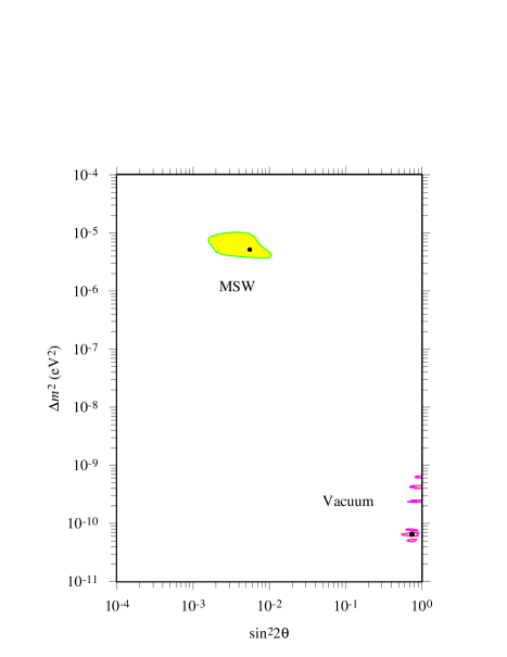
FIG. 12.: Allowed regions of neutrino parameter space for two-flavor oscillations into active neutrino species. The analysis uses the results of all solar neutrino experiments, including the constraints from the energy spectrum and zenith-angle dependence measured by Super-Kamiokande. The black circles are the best fit points and the shading shows the allowed regions at 99% confidence. Thee figure is based on calculations in Ref. [16].

More credible explanations for the solar neutrino deficit involve either matter-enhanced Mikheyev-Smirnov-Wolfenstein (MSW) neutrino oscillations, in which the solar $\nu_{e}$ oscillates into other flavor neutrinos or a sterile neutrino [16, 54, 55, 56], or vacuum oscillations [57, 16, 58]. For both of these possibilities, the allowed regions of $\Delta m^{2}-\sin^{2}2\theta$ parameter space determined from solar neutrino experiments for two-flavor oscillations into active neutrino species are shown in Fig. 12. The fit quality is about the same in both regions. There is also a fit with similar quality for MSW oscillations into sterile neutrinos, whose allowed region approximately coincides with the region shown for MSW oscillations with active neutrinos.

There are now very strong indications that the solar neutrino deficit has a particle physics explanation and is a consequence of neutrino mass. To fully unravel the solar neutrino story, however, will require more experiments, especially those with sensitivity to low-energy neutrinos or to neutrino flavor. SAGE continues to perform regular solar neutrino extractions every 6 weeks with $\sim 50$ tons of Ga and will continue to reduce its statistical and systematic uncertainties, thus further limiting possible solutions to the solar neutrino problem.

A Other Counting Systems

The counting systems have been designated by the numbers 1–6. The initial developmental work on system 1 [59, 60], which used the amplitude of the differentiated pulse (ADP) method [61] to separate ⁷¹Ge events from background, was done in Russia during the early 1980s. Based on this work, system 2 was developed at BNO during the years 1985–1988. System 2 was completed in 1989 and counted all but two first extractions through May 1992 (SAGE I). Counting system 5, which used the ADP method of rise time measurement, was used to count the other two first extractions during 1990 and 1991. During the summer of 1992, system 3, which has the capability to record the counter wave form, was brought on line; since that time, it has been used to count almost all first extractions. After the implementation of system 3 as the primary counting system, extensive upgrades to reduce backgrounds were performed on system 2 to enable SAGE to have low-noise counting capability in more than eight channels. The upgraded system is referred to as system 6. It has counted seven first extractions during SAGE II and III, mostly from low-mass samples of Ga, and has been used mainly for developmental work, such as testing proportional counters and counting cleanup extractions of gallium.

a Counting system 2

System 2 was a seven-channel system where each PC was counted in an independent passive shield; five of those channels had active shielding with NaI crystals. The passive shield consisted of an internal wall of tungsten (40–80 mm thick) or copper (20–30 mm thick) surrounded by lead (150 mm thick). The NaI events were recorded in coincidence mode with events from the proportional counters. Several of the performance characteristics of system 2 are given in Table VII.

b Counting system 6

Modifications to system 2 began during 1992 when system 3 became the primary acquisition system; the improvements were so extensive that it was redesignated as system 6. The counting system has seven channels of acquisition with independent passive shields for each proportional counter. Six channels have an active shield, which operates in coincidence mode with events in the proportional counter. A modified ADP method with the application of several differentiation time constants is used for rejection of point ionization events from backgrounds. System 6 became fully operational in early 1993. To give this system wave form recording capability a digitizing oscilloscope was added, but this improvement has never been fully implemented.

B Fourier transform of the wave form – $\textstyle R$

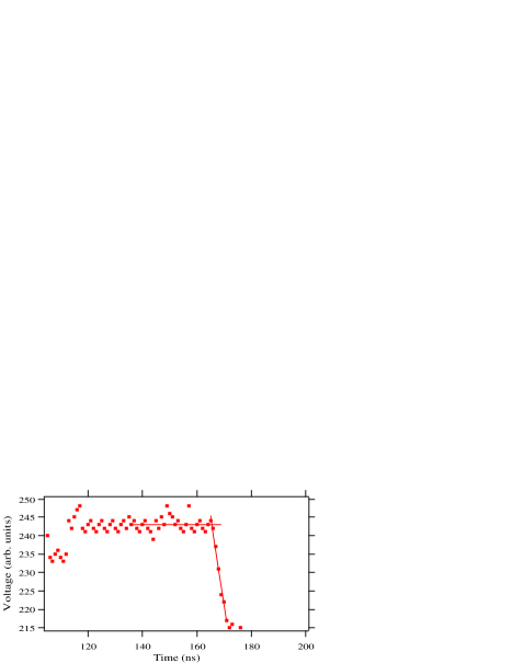
FIG. 13.: Determination of the time and dc offset of a candidate event.

In contrast to the $T_{N}$ method, the pulse offset is determined independently from the wave form. One uses the intersection point of two lines, the zero-slope line of the offset and the initial slope of the pulse, to obtain the onset position in time and voltage. The initial slope is defined as a certain number of points before and after the point at 20% of the maximum pulse height. The exact number of points to fit is determined individually for each pulse since the number of points available will depend on the pulse height. This region is chosen so that the points are sufficiently linear. Figure 13 illustrates graphically how the onset point is determined.

Two data runs with counters filled with ⁷¹Ge were used to check the energy offset from this wave form analysis determination. The runs were separated by three years and used different digitizer settings. The Gaussian centroid of each $L$ peak and $K$ peak was calculated, with each peak containing a few thousand counts. The extrapolated intercepts in energy are 0.005(6) keV and 0.022(8) keV using $L$- and $K$-peak energies of 1.17 keV and 10.37 keV. Given the energy resolution of our counters, the energy offset is effectively zero.

The algorithm for determining the pulse onset was checked using computer-simulated pulses, both with and without Gaussian noise. It correctly identifies the time offset to within 1 ns and the dc offset to within one channel. Those limits are, of course, dependent on the noise levels, but the levels used were approximately the same as for typical data. Thus, if each pulse is properly normalized to both zero time and dc offset, there is no need to apply an energy offset correction.

This technique uses the zero- and lowest-frequency values from a FFT to obtain measures of the energy and rise time of a pulse. The determination of the energy is straightforward from the definition of the Fourier transform,

$$F(\omega)=\int_{-\infty}^{+\infty}{f(t)e^{-i\omega t}dt}.$$ (B1)

At $\omega=0$, $F(\omega)$ equals the area under the curve $f(t)$, which in this case is the digitized wave form of the event convoluted with a Hanning windowing function. We select an integration time of 800 ns, which is the maximum time allowable given the variation in the time of pulse onset. In effect, this technique is equivalent to summing channels used with $T_{N}$ and is analogous to an ADC that integrates for 800 ns.

In a Fourier analysis, the rise time behavior of a typical pulse clearly will be a very-low-frequency component. Studies with actual ⁷¹Ge pulses and computer-simulated pulses generated with Eqs. (8) show that one can accurately identify several distinct features of the wave form. As expected, the dominant components are the lowest frequencies along with the random noise that spans all frequencies. One can identify structure as well; most of it originates from the intrinsic properties of the oscilloscope, such as dithering and the finite digitization size. One of the advantages of a Fourier analysis is that such structure appears at high frequencies and is well separated from the rise time information. The lowest, nonzero, real component $F(1)$ scales similarly to an ADP value but is independent of electronic offsets and high-frequency noise contributions to the pulse. Dividing it by the energy $F(0)$ of the pulse produces a parameter $R$ that is proportional to the inverse rise time. Thus, one can perform a complementary analysis of the data that is analogous to the ADP method but is based solely on the digitized pulse and is independent of any underlying assumptions of its functional form.

C RST method

In the standard analysis of our data we use the $T_{N}$ method and fit the observed pulse to Eq. 8. This function gives the correct description of the shape of the voltage pulse as recorded by the digital oscilloscope when the ionization produced in the proportional counter consists of a set of point ionizations evenly distributed along a straight track. Since ⁷¹Ge events are usually a single cluster of ionization, this method works satisfactorily to select ⁷¹Ge candidate events. It is, however, restricted to the particular form of ionization that is assumed, and gives a poor fit to other types of charge deposit in the counter, such as the combination of a point event from ⁷¹Ge $K$-electron capture followed by capture of the 9.3-keV x ray at some other location in the counter. To give us the capability to investigate all possible events that may occur in the counter, we have also developed a more general method which can analyze an event produced by ionization with an arbitrary distribution of charge. We call this the “restored pulse method” or “RST method” for short.

We begin with the measured voltage pulse $V(t)$ as recorded by the digitizer. For an ideal point charge that arrives at the counter anode wire, $V(t)$ has the Wilkinson form $V(t)=W(t)=V_{0}\ln(1+t/t_{0})$, provided the counter is ideal and the pulse processing electronics has infinite bandwidth. For a real event from the counter, with unknown charge distribution, $V(t)$ can in general be expressed as the convolution of the Wilkinson function with a charge collection function $G(t)$:

$$V(t)=W(t)\otimes G(t).$$ (C1)

The function $G(t)$ contains within it the desired information about the arrival of charge at the counter anode, coupled with any deviations of the counter or electronics from ideal response. Equation (C1) can be considered as the definition of $G(t)$.

To get the desired function $G(t)$, one must deconvolute Eq. (C1). To perform this deconvolution, we have found it mathematically convenient to use the current pulse $I(t)$, which is obtained by numerical differentiation of $V(t)$:

$$I(t) = \frac{dV}{dt}=\frac{d}{dt}[W(t)\otimes G(t)]$$ (C2)

$$= \frac{dW}{dt}\otimes G(t)=W^{{}^{\prime}}(t)\otimes G(t),$$ (C3)

where $W^{{}^{\prime}}(t)$ is normalized over the observed time of pulse measurement, $T_{\text{obs}},$ such that $\int_{0}^{T_{\text{obs}}}W^{{}^{\prime}}(t)dt=1$.

To deconvolute, we Fourier transform to the frequency domain and then use the theorem that convolution in the time domain becomes multiplication in the frequency domain [62]. This simply gives $I(f)=W^{{}^{\prime}}(f)G(f)$, which can be solved for $G(f)$. We then Fourier transform $G(f)$ back to the time domain to get the desired function $G(t)$. The energy of the event is given by $\int_{0}^{T_{\text{obs}}}G(t)dt$. The duration of the collection of ionization is given by the width of $G(t)$, which can be used as a measure of the rise time.

FIG. 14.: Analysis of typical ⁷¹Ge pulse by the RST method. See text for explanation.

An example of this procedure as applied to a typical ⁷¹Ge $K$-peak event is given in Fig. 14. This pulse has $T_{N}=3.9$ ns. The recorded voltage pulse after inversion and smoothing is given by $V(T)$ in the lower panel. The current pulse, obtained by numerical differentiation of the voltage pulse, is given by $I(t)$ in the upper panel. The deduced function $G(t)$ is also shown in the upper panel. It has a FWHM of about 15 ns, found to be typical for true ⁷¹Ge $K$-peak events. The integrated current pulse, which records the pulse energy, is given by $\int G(t)dt$ in the lower panel.

This method has the advantage that it can reveal the basic nature of the ionization in the counter for an arbitrary pulse. It is also capable of determining the pulse energy over a wider range than the $T_{N}$ method. A problem that has been found with this method in practice, however, is that when ⁷¹Ge data are analyzed one obtains multiple collection functions [i.e., $G(t)$ has several distinct peaks separated in time] more often than is expected from the known physical processes that take place in the counter. These multiple peaks are due to noise on the pulse and cutoff of the system frequency response at about 100 MHz. Attempts have been made to remove these extraneous peaks by filtering and smoothing the original pulse, but they have not been fully successful. Evidently we need faster electronics and a reduction in the noise level to be able to fully exploit this pulse shape analysis technique. As a result, we have only been able to use this method to select events on the basis of energy.

REFERENCES

- [1] R. Davis, Jr., in Frontiers of Neutrino Astrophysics, edited by Y. Suzuki and K. Nakamura (Universal Academy Press, Inc., Tokyo, 1993), p. 47; B. T. Cleveland, T. J. Daily, R. Davis, Jr., J. R. Distel, K. Lande, C. K. Lee, and P. S. Wildenhain, Nucl. Phys. B (Proc. Suppl.) 38, 47 (1995).
- [2] B. T. Cleveland, T. J. Daily, R. Davis, Jr., J. R. Distel, K. Lande, C. K. Lee, and P. S. Wildenhain, Astrophys. J. 496, 505 (1998).
- [3] J. N. Bahcall, M. H. Pinsonneault, and G. J. Wasserburg, hep-ph/9505425, Rev. Mod. Phys. 67, 781 (1995).
- [4] John N. Bahcall, Sarbani Basu, and M. H. Pinsonneault, astro-ph/9805135, Phys. Lett. B 433, 1 (1998).
- [5] A. S. Brun, S. Turck-Chièze, and P. Morel, astro-ph/9806272, Astrophys. J. 506, 913 (1998).
- [6] J. N. Bahcall and A. Ulmer, astro-ph/9602012, Phys. Rev. D 53, 4202 (1996).
- [7] J. N. Bahcall, Neutrino Astrophysics (Cambridge University Press, Cambridge, England, 1989).
- [8] Y. Fukuda et al., Phys. Rev. Lett. 77, 1683 (1996).
- [9] V. A. Kuzmin, Zh. Eksp. Teor. Fiz. 49, 1532 (1965) [Sov. Phys. JETP 22, 1051 (1966)].
- [10] Table of Isotopes, 8th ed., edited by V. S. Shirley (John Wiley and Sons, New York, 1996), p. 209.
- [11] J. N. Bahcall, hep-ph/9710491, Phys. Rev. C 56, 3391 (1997).
- [12] V. N. Gavrin, in Proceedings of the 18th International Conference on Neutrino Physics and Astrophysics (Neutrino 98), Takayama, Japan, 1998, edited by Y. Suzuki and Y. Totsuka. Nucl. Phys. B (Proc. Suppl.) 77, 20 (1999)..
- [13] W. Hampel, J. Handt, G. Heusser, J. Kiko, T. Kirsten, M. Laubenstein, E. Pernicka, W. Rau, M. Wojcik, Y. Zakharov, R. v. Ammon, K. H. Ebert, T. Fritsch, E. Henrich, L. Stielglitz, F. Weirich, M. Balata, M. Sann, F. X. Hartmann, E. Bellotti, C. Cattadori, O. Cremonesi, N. Ferrari, E. Fiorini, L. Zanotti, M. Altmann, F. v. Feilitzsch, R. Mößbauer, S. Wänninger, G. Berthomieu, E. Schatzmann, I. Carmi, I. Dostrovsky, C. Bacci, P. Belli, R. Bernabei, S. d’Angelo, L. Paoluzi, M. Cribier, J. Rich, M. Spiro, C. Tao, D. Vignaud, J. Boger, R. L.Hahn, J. K. Rowley, R. W. Stoenner, and J. Weneser, Phys. Lett. B 447, 127 (1999).
- [14] Karsten M. Heeger and R. G. H. Robertson, nucl-th/9610030, Phys. Rev. Lett. 77, 3720 (1996).
- [15] A. Yu. Smirnov, hep-ph/9809481, in Proceedings of the 18th International Conference on Neutrino Physics and Astrophysics (Neutrino 98), Takayama, Japan, 1998, edited by Y. Suzuki and Y. Totsuka. Nucl. Phys. B (Proc. Suppl.) 77, 98 (1999).
- [16] J. N. Bahcall, P. I. Krastev, and A. Yu. Smirnov, hep-ph/9807216, Phys. Rev. D 58, 096016 (1998).
- [17] Y. Fukuda et al., hep-ex/9812011, Phys. Rev. Lett. 82, 1810 (1999).
- [18] J. N. Abdurashitov, E. L. Faizov, V. N. Gavrin, A. O. Gusev, A. V. Kalikhov, T. V. Knodel, I. I. Knyshenko, V. N. Kornoukhov, I. N. Mirmov, A. M. Psukhov, A. M. Shalagin, A. A. Shikhin, P. V. Timofeyev, E. P. Veretenkin, V. M. Vermul, G. T. Zatsepin, T. J. Bowles, S. R. Elliott, J. S. Nico, W. A. Teasdale, D. L. Wark, J. F. Wilkerson, B. T. Cleveland, T. Daily, R. Davis, K. Lande, C. K. Lee, P. S. Wildenhain, M. L. Cherry, and R. T. Kouzes, Phys. Lett. B 328, 234 (1994).
- [19] J. N. Abdurashitov, E. L. Faizov, V. N. Gavrin, A. O. Gusev, A. V. Kalikhov, T. V. Knodel, I. I. Knyshenko, V. N. Kornoukhov, I. N. Mirmov, A. M. Psukhov, A. M. Shalagin, A. A. Shikhin, P. V. Timofeyev, E. P. Veretenkin, V. M. Vermul, G. T. Zatsepin, T. J. Bowles, S. R. Elliott, J. S. Nico, W. A. Teasdale, D. L. Wark, J. F. Wilkerson, B. T. Cleveland, T. Daily, R. Davis, K. Lande, C. K. Lee, P. S. Wildenhain, M. L. Cherry, and R. T. Kouzes, in Proceedings of the XXVII International Conference on High-Energy Physics, Glasgow, 1994, edited by P. J. Bussey and I. G. Knowles (Institute of Physics, Bristol, 1994), p. 965.
- [20] J. N. Abdurashitov, V. N. Gavrin, S. V. Girin, V. V. Gorbachev, T. V. Ibragimova, A. V. Kalikhov, N. G. Khairnasov, T. V. Knodel, V. N. Kornoukhov, I. N. Mirmov, A. A. Shikhin, E. P. Veretenkin, V. M. Vermul, V. E. Yants, G. T. Zatsepin, T. J. Bowles, J. S. Nico, W. A. Teasdale, D. L. Wark, M. L. Cherry, V. N. Karaulov, V. L. Levitin, V. I. Maev, P. I. Nazarenko, V. S. Shkol’nik, N. V. Skorikov, B. T. Cleveland, T. Daily, R. Davis, Jr., K. Lande, C. K. Lee, P. S. Wildenhain, Yu. S. Khomyakov, A. V. Zvonarev, S. R. Elliott, and J. F. Wilkerson, Phys. Rev. Lett. 77, 4708 (1996).
- [21] J. N. Abdurashitov, V. N. Gavrin, S. V. Girin, V. V. Gorbachev, T. V. Ibragimova, A. V. Kalikhov, N. G. Khairnasov, T. V. Knodel, V. N. Kornoukhov, I. N. Mirmov, A. A. Shikhin, E. P. Veretenkin, V. M. Vermul, V. E. Yants, G. T. Zatsepin, Yu. S. Khomyakov, A. V. Zvonarev, T. J. Bowles, J. S. Nico, W. A. Teasdale, D. L. Wark, M. L. Cherry, V. N. Karaulov, V. L. Levitin, V. I. Maev, P. I. Nazarenko, V. S. Shkol’nik, N. V. Skorikov, B. T. Cleveland, T. Daily, R. Davis, Jr., K. Lande, C. K. Lee, P. S. Wildenhain, S. R. Elliott, and J. F. Wilkerson, hep-ph/9803418, Phys. Rev. C. 59, 2246 (1999).
- [22] J. N. Bahcall, B. T. Cleveland, R. Davis, Jr., I. Dostrovsky, J. C. Evans, Jr., W. Frati, G. Friedlander, K. Lande, J. K. Rowley, R. W. Stoenner, and J. Weneser, Phys. Rev. Lett. 40, 1351 (1978).
- [23] I. R. Barabanov, E. P. Veretenkin, V. N. Gavrin, L. A. Eroshkina, G. T. Zatsepin, Yu. I. Zakharov, S. A. Klimov, T. V. Knodel, A. V. Kopylov, I. V. Orekhov, A. A. Tikhonov, and M. I. Churmayeva, in Proceedings of the Conference on Solar Neutrinos and Neutrino Astronomy, Homestake, 1984, edited by M. L. Cherry, K. Lande, and W. A. Fowler, AIP Conf. Proc. No. 126 (AIP, New York, 1985), p. 175.
- [24] A. I. Abazov, D. N. Abdurashitov, O. L. Anosov, O. V. Bychuk, S. N. Danshin, L. A. Eroshkina, E. L. Faizov, V. N. Gavrin, V. I. Gayevsky, S. V. Girin, A. V. Kalikhov, S. M. Kireyev, T. V. Knodel, I. I. Knyshenko, V. N. Kornoukhov, S. A. Mezentseva, I. N. Mirmov, A. V. Ostrinsky, V. V. Petukhov, A. M. Pshukov, N. E. Revzin, A. A. Shikhin, E. D. Slyusareva, A. A. Tikhonov, P. V. Timofeyev, E. P. Veretenkin, V. M. Vermul, V. E. Yants, Yu. I. Zakharov, G. T. Zatsepin, V. L. Zhandarov, T. J. Bowles, B. T. Cleveland, S. R. Elliott, H. A. O’Brien, D. L. Wark, J. F. Wilkerson, R. Davis, Jr., K. Lande, M. L. Cherry, and R. T. Kouzes, in Inside the Sun: Proceedings of the 121st Colloquium of the International Astronomical Union, Versailles, France, 1989, edited by G. Berthomieu and M. Cribier (Kluwer Academic, Dordrecht, 1990), p. 201.
- [25] E. P. Veretenkin, V. M. Vermul, V. N. Gavrin, I. I. Knyshenko, and I. N. Mirmov, Institute for Nuclear Research of the Academy of Sciences of the USSR Report No. P-0692, 1991.
- [26] E. P. Veretenkin, L. A. Eroshkina, S. M. Kireev, and L. A. Niselson, Institute for Nuclear Research of the Academy of Sciences of the USSR Report No. P-0553, 1987.
- [27] J. K. Rowley, GALLEX Internal Report No. GX-19, 1993.
- [28] W. Haxton, nucl-th/9804011, Phys. Lett. B 431, 110 (1998).
- [29] A. I. Abazov, O. L. Anosov, E. L. Faizov, V. N. Gavrin, A. V. Kalikhov, T. V. Knodel, V. N. Kornoukhov, S. A. Mezentseva, I. N. Mirmov, A. V. Ostrinsky, A. M. Pshukov, N. E. Revzin, A. A. Shikhin, P. V. Timofeyev, E. P. Veretenkin, V. M. Vermul, G. T. Zatsepin, T. J. Bowles, B. T. Cleveland, S. R. Elliott, H. A. O’Brien, D. L. Wark, J. F. Wilkerson, R. Davis, Jr., K. Lande, M. L. Cherry, and R. T. Kouzes, Phys. Rev. Lett. 67, 3332 (1991).
- [30] W. Hampel and L. Remsberg, Phys. Rev. C 31, 666 (1985).
- [31] H. Genze, J. P. Renier, J. G. Pengra, and R. W. Fink, Phys. Rev. C 3, 172 (1971); W. Neumann, in Proceedings of the International Conference on X-ray and Atomic Inner Shell Physics, Eugene, Oregon, August 1982 (unpublished).
- [32] E. Browne and R. B. Firestone, Table of Radioactive Isotopes (Wiley, New York, 1986).
- [33] J. N. Abdurashitov, A. O. Gusev, and V. E. Yants, in Proceedings Particles and Cosmology Workshop, Baksan Valley, Russia, edited by E. N. Alexeev, V. A. Matveev, Kh. S. Norov, and V. A. Rubakov, (World Scientific, Singapore, 1995), p. 70.
- [34] R. Kouzes and D. Reynolds, IEEE Trans. Nucl. Sci., 36, 846 (1989).
- [35] J. Va’vra, Nucl. Instrum. Methods Phys. Res. A 252, 547 (1986).
- [36] J. N. Bahcall, B. T. Cleveland, R. Davis, and J. K. Rowley, Astrophys. J. Lett. Ed. 292, L79 (1985).
- [37] S. R. Elliott, Nucl. Instrum. Methods Phys. Res. A 290, 158 (1990).
- [38] B. T. Cleveland, Nucl. Instrum. Methods Phys. Res. 214, 451 (1983).
- [39] B. T. Cleveland, Nucl. Instrum. Methods Phys. Res. A 416, 405 (1998).
- [40] V. N. Gavrin, V. N. Kornoukhov, and V. E. Yants, Institute for Nuclear Research of the Academy of Sciences of the USSR Report No. P-0703, 1991.
- [41] I. R. Barabanov, V. N. Gavrin, G. T. Zatsepin, I. V. Orekhov, and E. A. Yanovich, At. Energy, 47(4), 273 1979.
- [42] I. R. Barabanov, V. N. Gavrin, P. P. Prokopeva, and V. E. Yants, Institute for Nuclear Research of the Academy of Sciences of the USSR Report No. P-0559, 1987.
- [43] V. N. Kornoukhov, Ph.D. thesis, Institute for Nuclear Research of the Russian Academy of Sciences, Moscow, 1998 (in Russian).
- [44] V. N. Gavrin, S. N. Danshin, A. V. Kopylov, and V. E. Cherekhovsky, Institute for Nuclear Research of the Academy of Sciences of the USSR Report No. P-0494, 1986.
- [45] Charles Evans Associates report (unpublished).
- [46] Shiva Technolgies report (unpublished).
- [47] V. N. Gavrin, V. E. Gurentsov, V. N. Kornoukhov, A. M. Pshukov, and A. A. Shikhin, Institute for Nuclear Research of the Academy of Sciences of the USSR Report No. P-0698, 1991.
- [48] M. Cribier, B. Pichard, J. Rich, J. P. Soirat, M. Spiro, Th. Stolarczyk, C. Tao, D. Vignaud, P. Anselmann, A. Lenzing, C. Schlosser, R. Wink, and J. K. Rowley, Astropart. Phys. 6, 129 (1997).
- [49] O. G. Ryazhskaya and G. T. Zatsepin, in Proceedings of the Ninth International Conference on Cosmic Rays, London, 1965, (Institute of Physics, London 1965), Vol. 2, p. 987.
- [50] V. N. Gavrin and Yu. I. Zakharov, Institute for Nuclear Research of the Academy of Sciences of the USSR Report No. P-0560, 1987.
- [51] V. Berezinsky, G. Fiorentini, and M. Lissia, astro-ph/9509116, Phys. Lett. B 365, 185 (1996).
- [52] V. Berezinsky, astro-ph/9710126, in Proceedings of the 25th International Cosmic Ray Conference, Durban, South Africa, 1997, edited by M. S. Potgieter, B. C. Raubenheimer, and D. J. van der Walt, (World Scientific, Singapore, 1998), Vol. 8, p. 59.
- [53] Arnon Dar and Giora Shaviv, astro-ph/9808098, “Proceedings of the Conference on Astrophysical Plasmas: From Atomic Nuclei to Stars and Galaxies,” Haifa, Israel, 1998, Phys. Rep. 311, 115 (1999).
- [54] D. O. Caldwell, Int. J. Mod. Phys. A 13, 4409 (1998).
- [55] S. M. Bilenky, C. Giunti, and W. Grimus, hep-ph/9812360, Prog. Part. Nucl. Phys. 43, 1 (1999).
- [56] N. Hata and P. Lankacker, hep-ph/9705339, Phys. Rev. D 56, 6107 (1997).
- [57] P. I. Krastev and S. T. Petcov, hep-ph/9510367, Phys. Rev. D 53, 1665 (1996).
- [58] James M. Gelb and S. P. Rosen, hep-ph/9809508, Phys. Rev. D 60, 011301 (1999).
- [59] I. R. Barabanov, V. N. Gavrin, Yu. I. Zakharov, and A. A. Tikhonov, Institute for Nuclear Research of the Academy of Sciences of the USSR Report No. P-0319, 1983.
- [60] A. A. Gogin, V. L. Zhandarov, Yu. I. Zakharov, and A. A. Tikhonov, Institute for Nuclear Research of the Academy of Sciences of the USSR Report No. P-0320, 1983.
- [61] R. Davis, Jr., J. C. Evans, V. Radeka, and L. Rogers, in Proceedings of the 3rd International Conference on Neutrino Physics and Astrophysics (Neutrino 72), Balatonfüred, Hungary, 1972, edited by A. Frenkel and G. Marx, Vol. I, p. 51.
- [62] W. H. Press, B. P. Flannery, S. A. Teukolsky, and W. T. Vetterling, Numerical Recipes in C (Cambridge University Press, Cambridge, England, 1988), p. 400.