Non-gravitational heating in the hierarchical formation of X-ray clusters

Abstract

The strong deviation in the properties of X-ray clusters from simple scaling laws highlights the importance of non-gravitational heating and cooling processes in the evolution of proto-cluster gas. We investigate this from two directions: by finding the amount of ‘excess energy’ required in intra-cluster gas in order to reproduce the observed X-ray cluster properties, and by studying the excess energies obtained from supernovae in a semi-analytic model of galaxy formation. Using the insights obtained from the model, we then critically discuss possible ways of achieving the high excess specific energies required in clusters. These include heating by supernovae and active galactic nuclei, the role of entropy, and the effect of removing gas through radiative cooling.

Our model self-consistently follows the production of excess energy and its effect on gas halos. Excess energy is retained in the gas as gravitational, kinetic and/or thermal energy. The density profile of a gas halo is then selected according to the total energy of the gas. Our principle assumption is that in the absence of non-gravitational processes, the total energy of the gas scales as the gravitational energy of the virialized halo—a self-similar scaling law motivated by hydrodynamic simulations. This relation is normalized by matching the model to the largest observed clusters.

We model the gas distributions in halos by using a 2-parameter family of gas profiles. In order to study the sensitivity of results to the model, we investigate four contrasting ways of modifying gas profiles in the presence of excess energy. In addition, we estimate the minimum excess energy required in a fiducial cluster of around 2 keV in temperature by considering all available gas profiles. We conclude that the excess energies required lie roughly in the range 1–3 keV/particle.

The observed metallicities of cluster gas suggests that it may be possible for supernovae to provide all of the required excess energy. However, we argue that this scenario is only marginally acceptable and would lead to highly contrived models of galaxy formation. On the other hand, more than enough energy may be available from active galactic nuclei.

1 Introduction

Much progress has been made in recent years in the modelling of galaxy formation, partly in response to an unprecedented amount of new data, especially for galaxies at high redshift. This paper however aims to constrain the model from the high-mass end, by tackling the properties of X-ray clusters. This has the advantage that the results are insensitive to the detailed physics of star formation and feedback. Only a small fraction of the hot gas in clusters is able to cool in a Hubble time, so that any star formation has little effect on the structure of the gas halo. Since star formation and feedback are two of the least understood components of galaxy formation, this seems to be a natural approach to take.

On the other hand, X-ray clusters do contain a fossil record of the complex star-formation history of their progenitors. The amount of gas left in a cluster’s halo depends on the amount consumed in processes such as star formation. The heavy elements (or metals) observed in the gas are the result of enrichment by supernovae over billions of years. Like the metals, the energy injected into the gas by supernovae and active galactic nuclei (AGN) is retained in the gas if it is not radiated. We shall be particularly interested in this ‘excess energy’ that is retained in present day clusters. X-ray clusters therefore provide important constraints on the history of a large sample of baryons.

Broadly speaking, a complex physical system can be studied via numerical methods, e.g. N-body simulations, or via analytic calculations. In galaxy formation theory, the semi-analytic approach has come to refer to more than just an intermediate line of attack, but to a specific class of models that use the hierarchical merger tree as their starting point. In the Cold Dark Matter (CDM) model [Blumenthal et al. (1984)], small halos virialize first and progressively collapse into larger and larger halos. The merger tree follows the masses of these halos as a function of time. The evolution of the baryonic component in these halos—which comprises $\sim 1/10$ of the total mass—receives a simplified yet physical treatment that models processes such as cooling, star formation and supernova feedback, to name a few.

Although N-body simulations of dark matter (DM) clustering now provide perhaps the best understood piece in the jigsaw of how galaxies formed, the evolution of the baryonic component remains much less well understood. In both hydrodynamic+DM simulations and semi-analytic models (SAMs), many of the above gas processes need to be approximated by simple rules. Nevertheless, using SAMs, we are able to efficiently explore the unknown parameters in these processes, and study the range of behaviour in these systems. In this way, SAMs have achieved notable success in modelling many properties of galaxies [White & Frenk (1991), Kauffmann et al. (1993), Cole et al. (1994), Kauffmann & Charlot (1998), Baugh et al. (1998), Somerville & Primack (1998), Guiderdoni et al. (1998)].

In this paper, we investigate the effect of excess energy on the density profiles of gas halos, and thus on the properties of X-ray clusters. Excess energy is retained in the gas as thermal, gravitational and/or kinetic energy as it passes through a merger tree. Even if the gas is ejected from a halo, it is expected to recollapse into a larger halo at a later time, thus the excess energy is not lost. As a first approximation, the excess energy in a gas halo is given by the total energy obtained from non-gravitational heating, minus the energy lost via radiative cooling. By non-gravitational heating we refer to heating by sources such as supernovae and AGN. The total energy released by such sources (though not necessarily injected into or retained by the gas) comes to several keV per particle when averaged over all baryons in the universe. It therefore has the potential to strongly influence the properties of X-ray clusters and galaxies.

It has been known for some time that the match between theoretical predictions and the observed properties of X-ray clusters is significantly improved if we assume that the gas is ‘pre-heated’ in some way [Kaiser (1991)]. Hydrodynamic simulations without non-gravitational heating or cooling [Navarro et al. (1995), Bryan & Norman (1998)] obtain X-ray clusters that are approximately ‘self-similar’, in the sense that small clusters (with temperatures $\approx 2\times 10^{7}$ K) are similar to large clusters ($T\sim 10^{8}$ K) scaled down in size. (Note that densities do not change in such a scaling.) However, the gas halos of observed clusters are not self-similar. For example, the X-ray luminosities of small clusters are an order of magnitude less than those predicted by scaling down the luminosities of large clusters in this way. This suggests that the gas distributions of small clusters are less concentrated than in large clusters. In order to break the self-similarity of X-ray clusters, excess energy is generally required. Excess energy affects small clusters much more than large ones. It can make the gas distribution more extended, or even remove some gas from the halo. Different models for heating clusters and breaking their self-similarity have been studied by a number of authors [Kaiser (1991), Evrard & Henry (1991), Metzler & Evrard (1994), Navarro et al. (1995), Cavaliere et al. (1997), Wu et al. (1998), Ponman et al. (1999), Balogh et al. (1999), Loewenstein (1999), Pen (1999)].

In order to model the effect of excess energy on gas halos, it is necessary to have a continuous range of gas profiles to choose from. The gas profile with density proportional to $r^{-2}$ has been used successfully in many SAMs to model galaxies. However, it is too simple for modelling the properties of X-ray clusters. In particular, the core of the gas density profile has to be flattened in order to obtain results that match the data (Wu, Fabian & Nulsen 1998; WFN98). In WFN98 we introduced a family of isothermal gas profiles into our SAM. We assumed the gas to be in hydrostatic equilibrium inside potential wells given by Navarro, Frenk & White (1997; NFW97) density profiles. This family of gas profiles enabled us to increase the temperature of a gas halo uniformly, according to the excess energy in the gas. The main results from that paper are that we were able to fit the observed properties of X-ray clusters, including their gas fractions, metallicities, X-ray luminosity-temperature relation, temperature function, X-ray luminosity function and mass-deposition-rate function, by including excess energies of $\sim 1$ keV/particle.

However, for a given total energy possessed by the gas halo (the sum of its thermal and potential energies), the isothermal profile represents only one solution out of a continuous range of possible solutions. Furthermore, it is uncertain how heating modifies a gas halo, since that depends on details of how the heating occurred. We therefore need to test the sensitivity of results to the way that we modify the gas halo when excess energy is present. To do this, we extend the family of isothermal profiles by requiring that gas halos obey polytropic equations of state: $P\propto\rho_{\rm g}^{\gamma}$, where $P$ is pressure and $\rho_{\rm g}$ is gas density. Thus for a given potential well and total gas mass, the gas profile has two degrees of freedom, given by the parameter $\gamma$, which effectively specifies the shape of the temperature profile, and the normalization of the temperature profile. The isothermal profiles are retrieved when $\gamma=1$, while progressively steeper temperature gradients are obtained by increasing $\gamma$. We thus have the choice of increasing the temperature of a gas halo uniformly with radius or preferentially towards the centre, depending on the ‘heating model’ that is used. One of the main purposes of this paper is to constrain the level of excess energy that intra-cluster gas must have in order to match the observed properties of X-ray clusters. We then critically discuss possible ways of obtaining this level of heating.

The SAM used in this paper is based on that described by Nulsen & Fabian (1997, 1995; NF97 and NF95). A discussion of the main areas of difference with other SAMs is given in NF97. However, our study of X-ray clusters is not affected by such differences, as their X-ray properties depend almost entirely on their gas profiles only.

We use an open cosmology with $\Omega_{m}=0.3$ and no cosmological constant. A Hubble parameter of $H_{0}=50$ km s^-1 Mpc^-1 is assumed throughout. We assume that density fluctuations are described by a CDM power spectrum with a primordial spectral index of $n=1$ and normalized to give $\sigma_{8}=0.75$. In addition, we assume a baryon density parameter of $\Omega_{b}=0.02h^{-2}$ (where $H_{0}=100h$ km s^-1 Mpc^-1) based on big-bang nucleosynthesis and deuterium abundance measurements [Burles & Tytler (1998), Burles et al. (1999)]. For $h=0.5$, this implies $\Omega_{b}=0.08$ and an initial gas fraction of $\Omega_{b}/\Omega_{m}=0.27$.

1.1 Plan of the paper

The main results from our model are discussed in sections 5 and 6.

Section 5 investigates the excess energies required in X-ray clusters and the relevant parts of the model are described in sections 2.1, 3 and 4.

Section 6 discusses the amount of excess energy obtainable from supernova heating in our model and therefore requires knowledge of our star formation model as described in the rest of section 2.

In section 7 we discuss some effects not accounted for by our model that may possibly contribute to the excess energy. In the process, we give a more formal definition of excess energy and discuss the theory behind the concept in some detail.

Finally, in section 8 we discuss four possible scenarios for breaking the self-similarity of clusters, aiming to be as model-independent as possible. We consider three sources of energy: supernovae, AGN and preferential removal of gas by cooling. We also discuss the role of entropy in this problem (section 8.2) and emphasize that both energy and entropy are important in determining the final gas distribution. In section 9 we summarize our conclusions.

2 Brief Description of the Model

We begin with a general description of our model which can be applied to any reasonable gas and DM halo profiles. More detailed discussions of the gas processes and galaxy formation model can be found in NF95 and NF97, which assumed essentially the same physics as used here. In Appendix A we apply the rules given in this section to the set of density profiles that we shall adopt.

2.1 Merger trees

Merger trees of virialized halos are simulated using the Cole & Kaiser (1988) block model. In a ‘complete’ simulation, we use 20 levels of collapse hierarchy where the smallest regions are $1.5\times 10^{10}$M_⊙ in mass. In the block model, masses increase by factors of 2 between levels, so that the mass of the largest block is $7.9\times 10^{15}$M_⊙. This allows us to simulate the full range of structures from dwarf galaxies to the largest present-day clusters. However, if we are considering X-ray cluster properties only, it is $\sim 1000$ times faster to simulate only the top 10 levels of the collapse tree. The mass of the smallest regions is then $2^{10}\times 1.5\times 10^{10}=1.5\times 10^{13}$M_⊙. In such low-resolution simulations some additional assumptions need to be made, such as the value of the gas fraction left over from the formation of galaxies.

Since every collapse of a block (which corresponds to a major infall or merger) at least doubles the mass of the largest progenitor halo, a new halo is said to virialize with each collapse. The virial radius, $r_{200}$, is defined such that the mean density within it is 200 times the background density of an Einstein-de Sitter universe of the same age. The total mass of the halo inside $r_{200}$ is equal to the mass of the collapsed block. Likewise, the gas mass inside $r_{200}$ is the contribution from the entire block (unless the excess energy is so high that the gas halo is unbound). The new halo is given gas and DM density profiles, which allow the estimation of basic quantities such as the cooling time of the gas. From this starting point, the model proceeds to estimate the rate of star formation, supernova feedback, metal enrichment and other quantities that can be compared with observations. At the next merger, the properties of the progenitor halos (e.g. the mass of gas remaining) are then incorporated into the new halo.

A collapse which is followed too closely by a larger-scale collapse does not have time to form a virialized halo. It is therefore not counted as a separate collapse. We allow a minimum time interval between collapses which is parametrized as a multiple of the dynamical time. Our results are not sensitive to this parameter and it is given a value of 1.

2.2 Cold and hot collapses

For a gas halo to be considered hydrostatic, the gas at any radius has to remain still for at least the time it takes for sound to travel to the centre, which can itself be approximated by the free-fall time. As discussed in NF95, if the ratio of cooling time to free-fall time to the centre, $\tau=t_{\rm cool}/t_{\rm ff}$, is less than $\sim 1$, then the gas cools fast enough that it is not hydrostatically supported. It fragments and collects into cold clouds which we assume to form stars with a standard or slightly modified initial mass function (IMF). We refer to this as a cold collapse and the gas that takes part in it as cold gas.

When $\tau\mathrel{\hbox to0.0pt{\lower 3.0pt\hbox{$\sim$}\hss}\raise 2.0pt\hbox{$>$}}1$, a hydrostatic atmosphere of hot gas (at roughly the virial temperature) is able to form. In this case, a cooling flow occurs if some gas has time to cool before the next collapse. Cooling gas flows inward subsonically and remains hydrostatically supported. In clusters of galaxies, cooling flows are common and observations show that the gas that cools does not form stars with a standard IMF but must remain as very small, cold clouds or form low-mass stars [Fabian (1994)]. We refer to the product simply as baryonic dark matter (BDM). A possible mechanism for the formation of low-mass stars in cooling flows is described by ?), for the case of elliptical galaxies.

To estimate the masses of hot and cold gas produced in a collapse, we use the gas and total density profiles to estimate $t_{\rm cool}$ and $t_{\rm ff}$ as functions of radius. To simplify computation, $t_{\rm ff}$ is estimated using the free-fall time of a test particle in a uniform background density, i.e. $t_{\rm ff}=\sqrt{3\pi/16G\rho}$, where $G$ is the gravitational constant and the total density at the radius concerned is substituted for $\rho$. (This gives a slight overestimate of $t_{\rm ff}$, as density actually increases towards the centre.) We thus obtain $\tau(r)$, and compare it to a critical value, $\tau_{0}$, to determine if gas is hot or cold. In well-behaved cases $\tau$ increases monotonically with radius, so that there exists a unique radius $r_{\rm cf}$, inside of which gas is labelled as cold, outside as hot. As halo mass increases, the trend is for $r_{\rm cf}$ to move from outside the virial radius to the centre. In other words, cold collapse gives way to hot collapse as we go to more massive halos. This transition is quite abrupt and takes place over about one decade in mass.

From the above, it is clear that no single gas profile can always describe the gas halo. Cooling modifies the gas distribution, and in a cold collapse the assumption of hydrostatic equilibrium breaks down completely. However, the gas profile used in the model is only notional—defined as that obtained in a notional collapse with cooling ignored (Nulsen, Barcons & Fabian 1998). Used in this way, it allows us to estimate the behaviour of different subsets of gas. In the case of hot halos, if the part that has cooled is small compared to the whole, then the density and temperature of gas away from the cooled region do not change significantly as the halo reestablishes hydrostatic equilibrium. The original gas profile therefore gives reasonable estimates of bulk properties.

2.2.1 The criterion when excess energy is large

If the excess energy from heating is large enough to be comparable to the binding energy of the gas halo (as defined in section 4), then $\tau$ may not increase monotonically with radius (see Appendix A for examples). Such cases can account for a fair fraction of low-mass galaxies because of their smaller binding energies. This raises the question of whether gas with $\tau<\tau_{0}$ outside a core of gas where $\tau>\tau_{0}$ still ends up cold after collapse. Since the value of $\tau$ and its interpretation are approximate, we opt for a simple criterion in such cases, which determines whether all or none of the gas halo takes part in a cooling flow (Appendix A). We note that $\tau(r)$ is a fairly flat function of radius if the strongly heated gas halo is isothermal.

2.3 Star formation, supernova feedback, and cooling flows

Star formation is presumed to proceed rapidly in cold gas and leads quickly to type II supernovae. This is assumed to continue until the energy from supernovae is sufficient to eject the remaining gas in the halo to infinity, or until the cold gas is used up. If the gas halo is not ejected, supernova energy can modify the gas density profile by increasing the total energy of the remaining gas (see section 4). The effect of this is generally small but is included for consistency. The remaining gas, which is hot, may then take part in a cooling flow, depositing BDM if it manages to cool by the next collapse or the present day. For halos which contain only hot gas or cold gas, the situation is naturally simpler than described.

We only follow the production of type II supernovae (SNII) in our model. Precise knowledge of the IMF is not required, since we only need to know the number of SNII resulting from a certain amount of star formation. It is generally assumed that the progenitors of SNII are stars of mass $M>8$M_⊙. For a standard IMF (more precisely the Miller-Scalo IMF), we adopt the estimate of one SNII for every 80M_⊙ of stars formed with $M\leq 1$M_⊙ (Thomas & Fabian 1990). In the simulations, we make the simplification that stars with $M>1M_{\odot}$ are instantaneously recycled, so that only the total mass of stars with $M\leq 1$M_⊙ is recorded. This allows us to calculate the mass of stars remaining in present-day clusters. Since the lifetime of a star is approximately $10^{10}(M/M_{\odot})^{-3}$ years, the recorded stellar mass is a good approximation of this quantity.

[The above suggests that the amount of gas in a halo could be overestimated by the model, since in reality, stars of intermediate mass ($1M_{\odot}<M<8M_{\odot}$) recycle their gas as planetary nebulae on intermediate time scales. However, we find that in newly-formed halos, the stellar mass is almost always $\mathrel{\hbox to0.0pt{\lower 3.0pt\hbox{$\sim$}\hss}\raise 2.0pt\hbox{$<$}}1/10$ of the gas mass, so that the effect of recycled gas on the latter is small (halos of a few $10^{12}$M_⊙ are an exception, as $\sim 1/3$ of them have more stars than this). Another minor problem occurs when only a small fraction of the gas in a halo is cold, so that most of the cold gas forms stars. In this case, the assumption of instantaneous recycling can cause the amount of star formation to be overestimated (in the extreme, all of the cold gas can be converted into stars with $M<1M_{\odot}$). Fortunately, the fraction of stars formed in such situations is very small, so that the error in the stellar mass of present-day clusters is less than 1 per cent.]

In the simulations, we follow NF97 by boosting the above supernova rate by a factor of 5. Hence each SNII is associated with 16M_⊙ of stars formed with $M<1M_{\odot}$. This corresponds to using a flatter slope for the IMF. Since the bulk of star formation in our model occurs as massive bursts in dwarf galaxies, it should not be surprising to find that the IMF is modified under such circumstances.

To give an actual example, a power-law IMF with a slope of $x=0.9$ (the Salpeter IMF has $x=1.35$), and lower and upper cutoffs of 0.1M_⊙ and 50M_⊙, gives 1 SNII for every 15M_⊙ of stars with $M<1M_{\odot}$. (Results are not very sensitive to the upper cutoff, because very massive stars are rare.) Using this IMF, we can estimate the error in our assumption that the stellar mass of a present-day cluster is given by the stars with $M\leq 1$M_⊙. Suppose the stars in the cluster have an age of 5 Gyr instead of 10 Gyr, then the surviving stars would be given by $M<0.5^{-1/3}=1.26M_{\odot}$. For the above IMF, the stellar mass in the range $0.1M_{\odot}<M<1.26M_{\odot}$ is 11 per cent greater than that in the range $0.1M_{\odot}<M<1M_{\odot}$. The stellar mass of model clusters are therefore correct to $\sim 10$ per cent.

The energy per supernova available for the ejection of gas is parametrized as $4\times 10^{50}$$\epsilon_{\rm SN}$ erg [Spitzer (1978)]. Although the total energy released by a supernova is typically $\sim 10^{51}$ erg, a large fraction of this is likely to be radiated, especially if the supernova explodes in cold gas. Each SNII is assumed to release an average of 0.07M_⊙ of iron (Renzini et al. 1993). The solar iron abundance is taken to be 0.002 by mass (Allen 1976). Renzini et al. find that the average iron yield is fairly insensitive to the slope $x$ of the IMF. We note that a more recent compilation of average iron yields from a range of SNII models [Nagataki & Sato (1998)] shows a wider dispersion, ranging from 0.07 to 0.14M_⊙ of iron per SNII. However, most of these SNII models assume that the progenitor stars have solar metallicity, whereas the bulk of star formation in our model occurs in low metallicity dwarf galaxies. If we only consider the low metallicity SNII models, then the range narrows to about 0.07–0.09M_⊙ of iron per SNII.

When a new halo collapses, the mean iron abundance and mean excess specific energy ($E_{\rm excess}$) of the gas are calculated and assigned to the gas halo. The excess energy of a gas halo, as it name implies, is the increase in its total energy (defined below) relative to the total energy it would have in the absence of any non-gravitational processes. In the model it is approximated by the total energy injected by supernovae, minus the energy radiated in progenitor halos, over the history of the gas. If some gas is removed from the gas halo by a cooling flow, $E_{\rm excess}$ is assumed to stay the same for the remaining hot gas. The reduction in $E_{\rm excess}$ by radiative cooling is easily accounted for, since the cooled gas is either converted to stars/BDM, or is ejected from the halo by supernovae. Since we assume that the gas is always ejected at the escape velocity of the halo, the resulting value of $E_{\rm excess}$ is simply given by the binding energy of the gas halo (as defined below). Other mechanisms that may affect $E_{\rm excess}$ but are not accounted for by the model are discussed in section 7. In particular, if the gas is displaced by strong heating, this can lead to an extra ‘gravitational contribution’ to the excess energy, that is usually positive. Unfortunately, this contribution is in general difficult to compute (without hydrodynamic simulations) and is likely to be model-dependent as well. (The approximation to $E_{\rm excess}$ made by the model may be compared to the approximation made when inferring the clustering of mass from the clustering of galaxies, which is traditionally handled by a ‘bias parameter’.)

3 The distribution of total density in halos

We begin by specifying the total density profile of a halo, which allows us to derive the shape of the potential well. This is then used in the following section to derive gas density profiles.

From a series of N-body simulations in different cosmologies and with both CDM and power-law fluctuation spectra, Navarro, Frenk & White (1997; NFW) found that the density profiles of virialized halos obey a universal form, given by

$$\rho(r)={\delta_{c}\rho_{\rm crit}\over(r/r_{s})(1+r/r_{s})^{2}},$$ (1)

where $\rho_{\rm crit}=3H^{2}/8\pi G$ and $H$ is the Hubble parameter at the time of collapse. The characteristic density $\delta_{c}$ is calculated according to a prescription described in the Appendix of NFW. This method amounts to setting the scale density, $\rho_{s}=\delta_{c}\rho_{\rm crit}$, equal to 3000 times the background density when the halo was ‘assembled’, subject to an appropriate definition of this assembly time. The assembly time is a function of halo mass and redshift of virialization only (given the cosmology and fluctuation spectrum).

From the value of $\delta_{c}$ and the mean density of the halo within $r_{\rm 200}$, the scale radius $r_{s}$ is uniquely determined. Thus $\delta_{c}$ is the only ‘degree of freedom’ in the profile. For convenience, $x=r/r_{s}$ is often used to denote radius. The value of $x$ at the virial radius, $c=r_{\rm 200}/r_{s}$, is an important parameter known as the concentration.

[On a technical point, our model actually differs slightly from the original NFW prescription. This is because NFW defined the mean density of a halo to be $200\rho_{\rm crit}$, whereas we have chosen to follow the spherical collapse model more closely when calculating the mean density. By following their prescription for calculating $\delta_{c}$, we have preserved their explanation for its origin. However, quantities such as $r_{s}$ and $c$ will differ slightly.]

Figure 2: Scatter plot of concentration $c$ vs. halo mass. Halo masses take discrete values in the block model. Each mass bin contains a maximum of 100 points. Halos were selected randomly from the simulation regardless of redshift. The solid line gives the mean value of each mass bin, and the dotted lines are plotted one standard deviation from the mean.

We make the further approximation that the NFW profile describes the total density in a halo (i.e. including the gas density) and that it is truncated to zero for $r>r_{200}$. This allows us to derive the gravitational potential as a function of $x$:

$$\phi(x)=\alpha\left(-\frac{\ln(1+x)}{x}+\frac{1}{1+c}\right),$$ (2)

where $\alpha=4\pi G\rho_{s}r_{s}^{2}$.

To illustrate typical values of $c$ obtained in this model, Figure 2 shows a scatter plot of $c$ against halo mass for our choice of cosmology and fluctuation spectrum. For halos that collapse at a given redshift, $c$ increases substantially with decreasing mass, e.g. the steep upper edge of the distribution is given by halos that virialize at $z=0$. However, for a given mass bin, $c$ decreases with increasing redshift. As a result, the mean value of $c$ does not vary much with halo mass, because less massive halos are more likely to collapse at higher redshift.

4 THE DISTRIBUTION OF GAS IN HALOS

Given the NFW potential well (2) and the total gas mass within $r_{\rm 200}$, we make two further assumptions in order to calculate the gas density profile. The first is that the gas is in hydrostatic equilibrium, i.e.

$${{\rm d}P\over{\rm d}r}=-\rho_{\rm g}{{\rm d}\phi\over{\rm d}r},$$ (3)

and the second is that $P$ and $\rho_{\rm g}$ are related by some equation of state. For example, if we assume a perfect gas law and isothermality, then $P\propto\rho_{\rm g}$ and the only parameter is the temperature, $T$. Once $T$ is specified, the gas profile is uniquely determined. Below, we first describe the general procedure that we use to determine such parameters.

We refer to the gas profile obtained in the absence of excess energy as the default profile. Since the NFW profile is not self-similar (see Fig. 2), it is not possible to define a self-similar default profile for gas halos. In the absence of heating, it is common to assume that $\langle T\rangle$ is proportional to $\langle\sigma^{2}\rangle$ for the DM halo, where $\sigma$ is the velocity dispersion and the brackets denote some form of average. However, $\langle\sigma^{2}\rangle$ is non-trivial to compute for the DM halo, and we are more interested with the total energy of the gas halo than just its thermal energy, since any excess energy would be added to the former. In order to retain some level of self-similarity, we therefore postulate that the total specific energy of the gas halo, $E_{\rm gas}$, is proportional to the specific gravitational energy of the whole halo (which is modelled by the NFW profile):

$$E_{\rm gas}=K\frac{1}{M_{\rm tot}}\int\frac{1}{2}\rho_{\rm tot}\phi\,{\rm d}V,$$ (4)

where $E_{\rm gas}$ is defined by

$$E_{\rm gas}\equiv\frac{1}{M_{\rm gas}}\int\rho_{\rm g}\left(\frac{3kT}{2\mu m_{\rm H}}+\phi\right)\,{\rm d}V.$$ (5)

The above integrals are performed out to the radius $r_{\rm 200}$, $M_{\rm tot}$ and $M_{\rm gas}$ are the total mass and total gas mass respectively, and the total density $\rho_{\rm tot}$ is given by NFW density profile. The Boltzmann constant is denoted by $k$ and $\mu m_{\rm H}$ is the mean mass per particle of the gas. Note that $E_{\rm gas}<0$ in order for the gas halo to remain gravitationally bound.

The constant of proportionality $K$ is a parameter of the model. It is calibrated by requiring that the default profiles of the largest clusters approximate well those from X-ray observations. We match to the largest observed clusters because if heating does occur, we expect it to have least effect on them. Once $E_{\rm gas}$ is computed from (4), the gas profile is uniquely determined if it is selected from a family with only one parameter (e.g. the isothermal family). In general, a numerical procedure is required to search for the gas profile with the matching value of $E_{\rm gas}$. The X-ray clusters obtained in this way do closely follow the self-similar scaling relations for $M_{\rm tot}$, $T$ and $L_{\rm X}$.

We refer to the value of $|E_{\rm gas}|$ given by (4) as the binding energy. As its name implies, the binding energy is the excess specific energy required to unbind the gas halo.

When the excess specific energy, $E_{\rm excess}$, is non-zero, $E_{\rm gas}$ is increased accordingly:

$$E_{\rm gas}=K\frac{1}{M_{\rm tot}}\int\frac{1}{2}\rho_{\rm tot}\phi\,{\rm d}V+E_{\rm excess}.$$ (6)

This allows the heated gas profile to be found. In general, as $E_{\rm excess}$ increases, the gas temperature increases and the gas distribution becomes more extended (i.e. the density profile becomes flatter). Thus the excess energy goes into increasing both the thermal energy and the potential energy of the gas halo.

If an isothermal family of gas profiles is used, heating increases the temperature uniformly with radius. Frequently, properties such as the luminosity of an X-ray cluster or the amount of gas able to cool in a given time are sensitive only to the gas density near the centre. Therefore, if we increase the temperature preferentially towards the centre, then we can obtain the same changes in these properties for less excess energy. A convenient way of modelling non-isothermal profiles is to use a polytropic equation of state: $P\propto\rho_{\rm g}^{\gamma}$. There are then two degrees of freedom, represented by $\gamma$ and the constant of proportionality in the polytropic equation. Since there are two parameters, a continuous range of gas profiles now have the same value of $E_{\rm gas}$. Thus a further constraint is required to determine the gas profile uniquely.

A heating model is obtained by specifying

• the constraint used to determine the default profile, and

• the path in parameter space followed by the gas profile as $E_{\rm excess}$ increases.

In order to obtain a good match to the largest clusters, the parameter $K$ is allowed to depend on a). Thus, $K$ may also be regarded as part of the heating model. The specification of a heating model is of course artificial; in reality, the gas profile is determined by additional factors such as the gas entropy distribution and how shock heating occurs. In lieu of a more complex model, we shall use a few contrasting heating models to test the sensitivity our results.

4.1 A 2-parameter family of gas density profiles

We now derive the family of gas profiles used in our model, assuming a polytropic equation of state and a perfect gas law. If we first let $\gamma=1$, then $T$ is constant and equation 3 gives

$$\rho_{\rm g}(r)\propto\exp\left(-\frac{\mu m_{\rm H}}{kT}\phi(r)\right).$$ (7)

Inserting the expression (2) for the NFW potential yields

$$\rho_{\rm g}(r)\propto(1+x)^{\eta/x},$$ (8)

where $\eta=\mu m_{\rm H}\alpha/(kT)$ is a dimensionless parameter that characterizes the slope of the density profile. Recall that $\alpha$ is the characteristic gravitational potential of the NFW profile. The mean value of $\eta$ obtained by fitting this model to highly luminous X-ray clusters is approximately 10 [Ettori & Fabian (1999)].

For $\gamma\neq 1$, we use $P\propto\rho_{\rm g}^{\gamma}$ to eliminate $P$ in equation 3, and then use $\rho_{\rm g}^{\gamma-1}\propto T$ to get

$${{\rm d}\over{\rm d}r}\left(kT\over\mu m_{\rm H}\right)=-{\gamma-1\over\gamma}{{\rm d}\phi\over{\rm d}r}.$$ (9)

Substituting for the potential gives

$${T\over T_{200}}=1+{\gamma-1\over\gamma}\eta_{200}\left({\ln(1+x)\over x}-{\ln(1+c)\over c}\right),$$ (10)

where $\eta_{200}=\mu m_{\rm H}\alpha/(kT_{200})$ is the value of $\eta$ at the virial radius (where $x=c$). Thus, using $\gamma>1$ causes the temperature to increase monotonically towards the centre. Substituting $\rho_{\rm g}\propto T^{(1/\gamma-1)}$, we get

$${\rho_{\rm g}\over\rho_{\rm g,200}}=\left[1+{\gamma-1\over\gamma}\eta_{200}\left({\ln(1+x)\over x}-{\ln(1+c)\over c}\right)\right]^{1\over\gamma-1},$$ (11)

where $\rho_{\rm g,200}$ is the gas density at the virial radius. It is straightforward to show that this approaches the isothermal form (8) as $\gamma\rightarrow 1$. We henceforth use the parameters $\gamma$ and $\eta_{200}$ to specify the gas profile.

It is also useful to compute the ‘entropy’, $s=T/n_{e}^{2/3}$, where $n_{e}$ is the electron density, and $n_{e}\propto\rho_{\rm g}$. For our purposes, $s$ may simply be regarded as a label for the adiabat that the gas is on. For the gas to be stable to convection, the entropy must increase with radius. When $\gamma=5/3$, the entropy is constant with radius, thus the atmosphere is marginally stable to convection. Atmospheres with higher values of $\gamma$ and steeper temperature gradients convect to reduce the temperature gradient. Hence 5/3 is the maximum value of $\gamma$ used in the model. The minimum value used is $\gamma=1$. We do not use lower values of $\gamma$ as there is little evidence for the temperature in halos to increase with radius, both from X-ray cluster observations and hydrodynamic simulations.

Figure 4: Gas density profiles, with parameters representative of those obtained in heating models A and B (see Fig. 10 and text). The same total gas mass and NFW potential well were used throughout (we set $c=5$). The solid curve (the default profile for the purposes of this figure) uses $\eta_{200}=10$ and $\gamma=1$. The series of dotted profiles have $\gamma=1$ but decreasing values of $\eta_{200}$: namely $\eta_{200}=8.5$, 7.1, 6.0 and 5.1. These values were chosen so that their total specific energies, $E_{\rm gas}$, increase at regular intervals. The flattest profile, $\eta_{200}=5.1$, has zero total energy and is marginally bound. The series of dashed curves have the same total energies as the dotted curves, but have the following parameters: $(\eta_{200},\gamma)=(10,1.1)$, $(10,1.3)$, $(8.7,5/3)$ and $(6.8,5/3)$. Notice that for the same increase in $E_{\rm gas}$, increasing $\gamma$ has a greater effect on densities at small radii than reducing $\eta_{200}$. Finally, the dot-dashed curve uses $\gamma=1.2$ and $\eta_{200}=28$, and is representative of default profiles obtained in Models C and D.

Figure 6: As Fig. 4, but showing temperature profiles (note that the temperature scale is linear). Temperatures have been normalized so that the solid curve has a temperature of unity. Increasing $\gamma$ leads to steeper temperature gradients without changing the temperature at the virial radius ($x=c$). In contrast, reducing $\eta_{200}$ increases the temperature uniformly.

Figure 8: As Fig. 4, but showing ‘entropy’ profiles, given by the expression $T/\rho_{\rm g}^{2/3}$. Most of the profiles are quite steep, but increasing $\gamma$ (dashed curves) results in much flatter entropy profiles. Isentropic profiles are obtained when $\gamma=5/3$.

In Figs. 4, 6 and 8 we display the density, temperature and entropy profiles of a selection of gas halos covering a range of $\eta_{200}$ and $\gamma$ values. All other parameters, in particular the total gas mass and NFW potential well, have been kept constant. In each figure, the series of dotted curves and dashed curves represent two different ways of heating the gas halo represented by the solid curve. In each series, the value of $E_{\rm gas}$ was required to increase at regular intervals from that of the solid curve up to a value of zero. Hence the gas halo with the most energy in each series is only marginally bound. By comparing the two series it is evident that profiles with the same total energy can differ significantly.

4.2 Profile selection: the heating models

4.2.1 The default profile

The first step is to determine the default profile. In a 2-parameter family of gas profiles, a profile can be specified by the value of $E_{\rm gas}$ and one further constraint. We shall consider two different constraints for selecting default profiles: $\gamma=1$ or $\gamma=1.2$, depending on the heating model. The former yields isothermal gas halos in the absence of heating, and is motivated by its simplicity. The latter is motivated by the temperature profiles of X-ray clusters measured by Markevitch et al. (1998), who approximated their results with a polytropic index of 1.2–1.3. For each constraint, we need to calibrate the parameter $K$ used in equation 4.

We calibrate $K$ by matching the model clusters obtained with $E_{\rm excess}=0$ to the largest observed clusters. We do not attempt to estimate $K$ theoretically, as it is our opinion that $E_{\rm gas}$ depends on how the collapse occurred in detail. For example, how the gas collapsed relative to the dark matter affects how much energy was transferred between the two components. [However, we do assume that such processes result in the scaling law expressed in (4).]

To calibrate $K$ for the case of $\gamma=1$, we use the results of Ettori & Fabian (1998), who fitted the surface brightness profiles of 36 X-ray clusters with $L_{\rm X}\mathrel{\hbox to0.0pt{\lower 3.0pt\hbox{$\sim$}\hss}\raise 2.0pt\hbox{$>$}}10^{45}$ erg s^-1. When fitting to avoid any cooling flow region, they obtain a mean value of $\eta=10.29$ with an rms scatter of 1.55. (Since the temperature is constant, $\eta$ and $\eta_{200}$ are the same.) In order to match this we set $K=1.2$, which gives a mean value of $\eta=10.5$ in the corresponding model clusters. However, the scatter of $\eta$ in our model is only $\sim 0.5$. If we now set the gas fraction of clusters equal to 0.17 (the mean value obtained by [Evrard (1997)] and [Ettori & Fabian (1999)], assuming $h=0.5$), we find that the model clusters naturally follow the observed $L_{\rm X}-T$ relation for clusters more luminous than $2\times 10^{45}$ erg s^-1 [Allen & Fabian (1998a)]. (We refer to bolometric luminosities throughout.) Note that this fit is possible because the largest observed clusters roughly follow the self-similar relation $L_{\rm X}\propto T^{2}$, instead of the steeper relation obeyed by smaller clusters.

Turning to the case of $\gamma=1.2$, we note that compared to the isothermal profiles these are almost always poorer fits to the surface brightness profiles of real clusters [Ettori & Fabian (1999)]. Hence for this case we calibrate $K$ by simply matching the $L_{\rm X}-T$ relation measured by ?). As above, we set the gas fraction of all clusters equal to 0.17. We find that $K=1.5$ results in an $L_{\rm X}-T$ distribution that best fits the data. The resulting clusters have $\eta_{200}\approx 28$. An example of such a profile is shown in Figs. 4 to 8 as dot-dashed curves, for comparison with the solid curves ($\gamma=1$ and $\eta_{200}=10$). Notice that although the two density profiles have different shapes, they roughly follow each other and intersect at two points. [The higher value of $\eta_{200}=28$ merely implies that the temperature at $r_{200}$ is lower by a factor of 2.8 compared to the $\eta_{200}=10$ case.]

Since $\gamma$ is fixed for both types of default profile, it is not hard to show that $\eta_{200}$ is a function of the NFW concentration $c$ only. We find that it is only a weakly increasing function of $c$ in both cases. Since the model clusters have a relatively small scatter in $c$ and $\eta_{200}$, they are close to self-similar when heating is absent.

4.2.2 The heated profile

Figure 10: A schematic diagram of how gas profiles are selected in each heating model. The first step is to find the default profile: depending on the heating model it has either $\gamma=1$ or $\gamma=1.2$; $\eta_{200}$ is then determined by requiring that the total specific energy, $E_{\rm gas}$, satisfies (4). (Note that the parameter $K=1.2$ for Models A and B, and $K=1.5$ for Models C and D.) The filled circles give only the approximate positions of default profiles, since $\eta_{200}$ depends on the NFW concentration $c$. The heated profile is found in the second step: any excess specific energy increases $E_{\rm gas}$ accordingly, and may increase the temperature uniformly (Models B and D), or increase the temperature preferentially towards the centre (Models A and C; these are modified to accommodate the upper limit of $\gamma=5/3$ when heating is very strong).

When excess energy is present, the default profile is modified to give the heated profile. We model this in two ways: by decreasing $\eta_{200}$ while keeping $\gamma$ constant, or by increasing $\gamma$ while keeping $\eta_{200}$ constant. The former has the effect of increasing the temperature at all radii by the same amount (to see this, multiply equation 10 by $T_{200}$ and note that $\eta_{200}T_{200}$ remains constant). The latter steepens the temperature gradient while ensuring that the temperature at $r_{200}$ stays constant, so that heating is concentrated towards the centre.

Since there are two types of default profile, we have four heating models in total. These are summarized in Fig. 10. Models A and B have default profiles with $\gamma=1$ and Models C and D have default profiles with $\gamma=1.2$. Heating increases $\gamma$ in Models A and C, but reduces $\eta_{200}$ in Models B and D.

There are a few loose ends to tie up. If the excess energy is so high that $E_{\rm gas}>0$, then the gas is not bound and it does not form a halo. However, for Models A and C, the gas halo may still be bound when $\gamma$ has increased to 5/3. Therefore, to increase $E_{\rm gas}$ further we reduce $\eta_{200}$ instead, as shown in Fig. 10.

5 THE EXCESS ENERGIES REQUIRED IN X-RAY CLUSTERS

In this section, we present the cluster results obtained with each of the four heating models. Since we are concerned solely with clusters here, the parameter $\tau_{0}$ and the star formation model play almost no part in the results. (No cold collapse occurs in the model clusters for all reasonable values of $\tau_{0}$.)

The simulations are ‘low resolution’ in the sense that they only use the top 10 levels of the collapse tree (section 2.1). Hence, the smallest regions have masses of $1.5\times 10^{13}$M_⊙. Each simulation used a total of 10000 realisations of the merger tree. We set the gas fraction of every cluster equal to 0.17 [Evrard (1997), Ettori & Fabian (1999)] for definiteness. The formulae used to calculate bolometric luminosity $L_{\rm X}$, emission-weighted temperature $T$ and the instantaneous mass deposition rate, $\dot{M}$, are given in Appendix A. All quantities were evaluated at $z=0$.

One simulation was performed for each heating model, and in each case all of the clusters were given a constant excess specific energy. For each heating model, we found the excess specific energy that best fit the data by matching to the $L_{\rm X}-T$ relation of David et al. (1993) in the first instance.

Table 2: Best fitting values of excess energy for each heating model, obtained by matching to the $L_{\rm X}-T$ relation measured by David et al. (1993). Excess energy per particle is calculated as $(\mu m_{\rm H}\,\Delta E_{\rm gas})$.

Heating Model	Excess Energy (keV/particle)
A	1.8
B	2.8
C	2.2
D	3.0

Figure 12: Contour plot of the cluster X-ray luminosity-temperature distribution obtained from Model A, with heating included at the level given in Table 2. The contours are spaced at equal logarithmic intervals. The long straight line is the best fit (for bolometric luminosities) taken from David et al. (1993). The extent of the line corresponds roughly to the extent of the data.

Figure 14: Same as Fig. 12 but using Model B.

Figure 16: Same as Fig. 12 but using Model C.

Figure 18: Same as Fig. 12 but using Model D.

The best-fitting excess energy for each heating model is given in Table 2. The resulting $L_{\rm X}-T$ distributions are displayed in Figs 12 to 18. The slopes of the distributions given by Models B and D are slightly steeper than the observed slope. This suggests that we need to relax our assumption of a constant $E_{\rm excess}$ for all clusters. It is also evident that the $L_{\rm X}-T$ distributions flatten slightly at high temperatures, tending to $L_{\rm X}\propto T^{2}$, in agreement with the largest observed clusters ([Allen & Fabian (1998a)]).

Recall that we calibrated the largest clusters to match the $L_{\rm X}-T$ relation of Allen & Fabian when heating is absent. The results thus confirm that the largest clusters are least affected by the excess energy (see also Fig. 1 in WFN98). However, the hottest clusters shown are in fact about a factor of 1/3 less luminous than before heating. We do not attempt to correct for this relatively small discrepancy. It is possible that in reality $E_{\rm excess}$ would be more diluted, i.e. smaller than we have assumed, in the largest clusters.

As expected, Models A and C require less heating than the other models, because they concentrate heating towards the centre of clusters, where most of the luminosity comes from. In addition, Models C and D require slightly more excess energy than Models A and B, respectively. Nevertheless, the highest excess energy in Table 2 is only about 50 per cent more than the lowest, over a set of very different heating models.

Figure 20: The X-ray luminosity functions given by all four heating models. The model results are plotted as follows: Model A: solid line, Model B: dashed line, Model C: dot-dashed line, Model D: dotted line. The curve is the best-fitting Schechter function for the ROSAT Brightest Cluster Sample bolometric luminosity function (Ebeling et al. 1997).

Figure 22: The X-ray temperature functions given by all four heating models, plotted with the same line styles as in Fig. 20. The straight line is the power law fit obtained by Edge et al. (1990).

Figure 24: The mass deposition rate functions (plotted cumulatively) for all four heating models, plotted with the same line styles as in Fig. 20. The jagged line is the same function taken from Peres et al. (1997), modified by using a cluster age of 6 Gyr.

We display the X-ray luminosity function, temperature function and mass deposition rate ($\dot{M}$) function from the same simulations in Figs. 20, 22 and 24, respectively. In each plot we have used a different line for each heating model. Superimposed on each plot is the observed data, as described in the captions. The same remarks regarding the simulated and observed $\dot{M}$ functions made in the previous section apply here. (However, the exclusion of clusters cooler than $2\times 10^{7}$K has practically no effect on the $\dot{M}$ functions simulated here, for most gas halos below this temperature have been unbound.)

The luminosity and temperature functions obtained with all four heating models give good fits to the data. However, the model $\dot{M}$ functions give relatively poor fits.

Models C and D give particularly poor fits where $\dot{M}>100$M_⊙ y^-1. This is because the mass deposition rate of large clusters are too high in these models. This can be attributed to the flatter cores of their gas density profiles. The poor performance of Models C and D support the result that the $\gamma=1.2$ gas profiles are relatively poor fits to the surface brightness profiles of large clusters compared to the $\gamma=1$ profiles [Ettori & Fabian (1999)].

Models A and B show a deficit of clusters with small cooling flows ($\dot{M}=10$–100M_⊙ y^-1). The main reason for the deficit is because the excess energies are now too high for the smallest clusters. We have repeated the simulation for Model B using lower excess energies in clusters less massive than $246\times 10^{12}$ M_⊙. The excess energies are given in Table 4; they increase steadily with mass up to $246\times 10^{12}$ M_⊙. The resulting $L_{\rm X}-T$ distribution and $\dot{M}$ function are shown in Figs. 26 and 28, respectively. Both show a better match to the data than before. The new $\dot{M}$ function has an increased number of small cooling flows, and the new $L_{\rm X}-T$ distribution reaches to lower temperatures (due to the reappearance of $\sim 2$ keV clusters, which were previously unbound).

Table 4: Table of excess energies used with Model B to improve the mass deposition rate function, which is shown in Fig. 28.

Halo Mass ($10^{12}$M⊙)	Excess Energy (keV/particle)
$\geq 246$	2.8
123	2.3
61	1.9
35	1.5
15	1.1

Figure 26: As Fig. 14, but using excess energies which increase with halo mass, as given in Table 4. Model B was used. Previously unbound groups now appear at temperatures below 2 keV.

Figure 28: As Fig. 24 but for Model B only, using increasing excess energies with halo mass as given in Table 4. The number of small cooling flows has increased, improving the fit to the data.

If it is true that $E_{\rm excess}$ increases with cluster mass, then this may be hard to reconcile with heating by supernovae, because we then expect $E_{\rm excess}$ to become more diluted with increasing halo mass (see section 6). In this case, a significant amount of energy injection would have to occur in clusters themselves (possibly by AGN). However, we note that this result is somewhat model-dependent, for it is possible to avoid it by combining different heating models. If large clusters are heated preferentially towards the centre (as in Model A) but small clusters are heated more uniformly (as in Model B), then it is possible that an excess energy of roughly 1.8 keV/particle across all clusters could satisfy all the data (see Table 2 and 4). Such a scenario may result from a characteristic scale in the spatial distribution of the heat source (supernovae or AGN). Alternatively, a strong wind may distribute its energy more efficiently through a small (proto-)cluster, because the cluster is closer to being unbound, i.e. it is more disturbed.

5.1 Using all available gas profiles

By using all the available gas profiles in the 2-parameter family (i.e. independently of any heating model), we have also found the minimum excess energy required to put a fiducial cluster on the observed $L_{\rm X}-T$ relation.

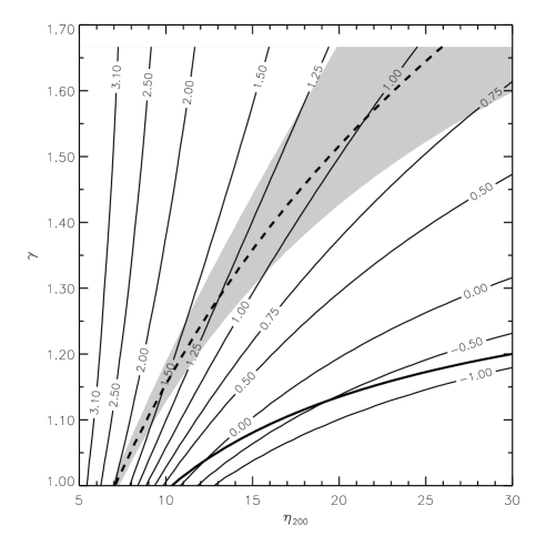
Figure 30: Contour plot in parameter space for a fiducial cluster of mass $1.23\times 10^{14}$ M_⊙, collapsing at $z=0$ with a gas fraction of 0.17. The dashed curve gives the parameters of gas halos that lie on the best-fitting $L_{\rm X}-T$ relation obtained by David et al. (1993), and gas halos in the shaded region lie within the region of uncertainty of this relation. The thin contours are labelled by excess energy (keV/particle), measured relative to an isothermal default profile (as in Models A and B). The profile that requires the least excess energy to match the $L_{\rm X}-T$ relation is given by $\gamma=5/3$ and $\eta_{200}=26$. It has an excess energy of 0.95 keV/particle. The thick solid line roughly sweeps out the positions of other possible default profiles (see text).

We considered the specific case of a halo of mass $1.23\times 10^{14}$ M_⊙, which virializes at $z=0$ with a gas fraction of 0.17. Such a cluster has a temperature of around 2 keV, depending on the amount of heating. To obtain the NFW profile we assumed the same cosmology as before. The problem was structured as follows. We first found the locus of points in $(\eta_{200},\gamma)$-space which put the cluster on the observed $L_{\rm X}-T$ relation. From these points we then found the one which had the least excess energy. However, the gas profile specified by $(\eta_{200},\gamma)$ only tells us the value of $E_{\rm gas}$—to compute $E_{\rm excess}$ we also need the ‘default’ value of $E_{\rm gas}$, i.e. when heating is absent. In what follows, we assume that the default value of $E_{\rm gas}$ is given by equation 4 with $K=1.2$ (as in Models A and B).

Fig. 30 shows contours of excess energy in parameter space, labelled in keV/particle. The gas halo becomes unbound for excess energies above 3.1 keV/particle. The dashed curve gives the parameters of gas halos that lie on the best-fitting power law to the observed $L_{\rm X}-T$ distribution [David et al. (1993)]. The shaded area contains gas halos that lie within the $1\sigma$ region of uncertainty for this best-fit. Note that it represents the uncertainty in the mean properties of X-ray clusters, and should not be confused with the dispersion in the $L_{\rm X}-T$ relation. From the plot, the gas profile with $\gamma=5/3$, $\eta_{200}=26$ requires the least excess energy to match the best-fit relation. It has an excess energy of 0.95 keV/particle. If the shaded region is taken into account, the minimum excess energy is roughly 0.7 keV/particle. It should not be surprising that the above profile is marginally stable to convection. We ‘save energy’ by concentrating the heating where it makes the most difference, i.e. near the centre, but convection limits the extent to which we can do this. The gas halo that requires the least heating is therefore the one with the isentropic atmosphere. This suggests that the $\gamma=5/3$ profile probably requires the least heating among all possible gas profiles.

Figure 32: Similar to Fig. 30, showing also contours of entropy at a radius of $0.1r_{200}$ (dotted lines). The contour labels give $s=T/n_{e}^{2/3}$ in units of keV cm².

A similar plot displayed in Fig. 32 shows contours of entropy (given by $s=T/n_{e}^{2/3}$) at a radius of $0.1r_{200}$. The entropy varies significantly along the dashed line, from around 200 keV cm² to 600 keV cm². The plot shows that the energy requirements are reduced if heating raises the entropy as much as possible. (We discuss this further in section 8.2.) The model entropies may be compared to the results of ?), who measured the entropies of groups and clusters at this radius in order to avoid possible cooling flows. However, these authors used emission-weighted temperatures to compute the entropy, whereas we have used radial-resolved temperatures. When this is accounted for, the above range of entropies are all consistent with the data.

So far we have assumed that in the absence of heating $E_{\rm gas}=-3.1$ keV/particle, as given by equation 4 using $K=1.2$. If we use $K=1.5$ instead (as in Models C and D), then the default value of $E_{\rm gas}$ becomes $1.5/1.2\times(-3.1)\approx-3.9$ keV/particle. As this is lower than before, all excess energies are increased by 0.8 keV/particle. We can generalize further by considering what parameters the cluster would need in order to lie on the self-similar relation $L_{\rm X}\propto T^{2}$ normalized to the largest observed clusters [Allen & Fabian (1998a)]. The gas profiles which satisfy this relation are given by the thick solid line in Fig. 30. As expected, it passes close to the points $(\eta_{200},\gamma)=(10,1)$ and (28,1.2), where the default profiles of our heating models are found. Thus the thick line roughly sweeps out the locations of possible default profiles. By assuming a $\gamma=1$ default profile in the above analysis, we obtained the highest default value of $E_{\rm gas}$, and therefore the lowest possible excess energies.

6 THE EFFECT OF SUPERNOVA HEATING

In this section, we investigate the amount of excess energy obtainable from supernova heating. Complete simulations with 20 levels of collapse hierarchy were performed with Models A and B. Each simulation used 100 realisations of the merger tree. Below, we begin by setting the parameters of the galaxy formation model.

6.1 Setting the model parameters

There are three parameters that remain to be set. They are the critical ratio of cooling time to free-fall time, $\tau_{0}$, the efficiency of supernova feedback, $\epsilon_{\rm SN}$, and the boost in the rate of supernovae. As mentioned in section 2.3, we assume that supernova rates are boosted by a factor of 5 for this work. Intuitively, this should increase the amount of supernova heating; however, we shall demonstrate that the resulting excess energies are quite insensitive to this parameter. All three parameters are kept constant in each simulation.

We assume an initial gas fraction of 0.27 (section 1). Unless stated otherwise, the resulting X-ray clusters have a mean gas fraction of 0.17 and a scatter of about 0.01, in agreement with the gas fraction used in the previous section.

6.1.1 Setting $\epsilon_{\rm SN}$

The feedback parameter $\epsilon_{\rm SN}$ controls the amount of star formation, which can be characterized by the fraction of gas turned into stars by the present day. Using the Coma cluster as a large sample of baryons, the mass ratio of hot gas to stars inside a radius of $1.5h^{-1}$ Mpc is about 15, assuming $h=0.5$ [White et al. (1993)]. In order to match this, we set $\epsilon_{\rm SN}$=0.3 for Model A and $\epsilon_{\rm SN}$=0.25 for Model B. We find that the required value of $\epsilon_{\rm SN}$ is almost independent of the value of $\tau_{0}$, unless $\tau_{0}$ takes an ‘extreme’ value ($\sim 10$ times greater or smaller than 1). In fact, a much larger fraction of baryons is converted into BDM than into stars (as can be seen from the primordial and cluster gas fractions). Most of the BDM is formed in the halos of massive galaxies and small groups.

6.1.2 Setting $\tau_{0}$

The parameter $\tau_{0}$ controls the transition from cold to hot collapse. From its definition, we know that $\tau_{0}\sim 1$. However, we consider a range of values: $\tau_{0}=1$, 0.4, and an extremely low value of 0.1, to illustrate its effect on the resulting excess energies. Table 6 lists the three sets of parameters used in the simulations.

Table 6: The values of $\epsilon_{\rm SN}$ and $\tau_{0}$ used with Models A and B.

	$\epsilon_{\rm SN}$	$\tau_{0}$
Model A	0.3	1.0
Model B	0.25	0.4
Model B	0.15	0.1

6.2 The excess energies from supernova heating

Figure 34: Scatter plot of excess energy vs. halo mass, using Model A. Each mass bin contains a maximum of 100 points. Halos were selected randomly from the simulation regardless of redshift. The solid line gives the mean value of each mass bin, and the dotted lines are plotted one standard deviation from the mean.

Figure 36: As Fig. 34, but showing the magnitude of the binding energy vs. halo mass. Note that the energy is now plotted logarithmically.

Figure 38: As Fig. 34, but showing the ratio of excess energy to binding energy. The dip in the mean for the lowest mass bins is caused by halos which have zero excess energy. This can only occur when a halo has no progenitors. Therefore, the dip is an artifact of the finite mass resolution. Notice that the finite points in the second lowest mass bin already have a similar distribution to higher mass bins.

For Model A, a scatter plot of excess energies vs. halo mass is displayed in Fig. 34, along with the mean and standard deviation for each mass bin. All of the scatter plots in this section were generated by randomly selecting up to 100 halos for each mass, regardless of redshift (only the most massive halos have less than 100 points plotted, because they are so rare). Up to a mass of $\sim 10^{12}$M_⊙, the excess energies clearly increase with mass. Above $\sim 10^{12}$M_⊙, star formation gives way to cooling flow behaviour, so that the mean excess energy changes little. However, the scatter reduces significantly due to an averaging effect. A gradual decrease in excess energy can be detected in the most massive halos, due to dilution by the accretion of primordial gas.

The ratio of excess energy to binding energy gives a measure of the excess energy’s ability to change the gas distribution. Recall that we define the binding energy to be equal to $|E_{\rm gas}|$ in the absence of heating. Fig. 36 shows a corresponding plot of binding energy for the same simulation as above. The ratio of excess energy to binding energy is displayed in Fig. 38. It has a strict upper limit of 1, above which gas halos are not bound. The distributions of points in mass bins below $\sim 10^{12}$M_⊙ are very similar and lie roughly in the range 0.2–0.6. The lowest mass bins are an exception because some of their halos have no excess energy at all; this causes the mean to dip for the lowest bins. As explained in the caption, this is purely an artifact of the finite mass resolution.

The approximately scale-invariant behaviour below $\sim 10^{12}$M_⊙ can be understood as follows. Below a certain halo mass, almost all of the galaxies produce sufficient supernova feedback to eject their gas. In addition, the gas is always ejected with excess energy equal to the binding energy of the host halo (for the model assumes that the gas is ejected at the escape velocity). As a result, for halos in, or slightly above, the said mass range, the ratio of excess energy to binding energy simply reflects the ratio of the binding energies of its progenitors to itself (ignoring the dilution of excess energy by primordial gas for simplicity). The similarity in the distribution of points in each mass bin (below $\sim 10^{12}$M_⊙) simply implies that these ratios do not change much with mass.

For halos $\mathrel{\hbox to0.0pt{\lower 3.0pt\hbox{$\sim$}\hss}\raise 2.0pt\hbox{$>$}}10^{12}$M_⊙, the ratio drops dramatically due to the cessation of star formation. Above $10^{14}$M_⊙—in the regime of X-ray clusters—the excess energies have hardly any effect on the gas halos.

Figure 40: The ratio of excess energy to binding energy obtained from Model B, using $\tau_{0}=0.4$ and $\epsilon_{\rm SN}$=0.25. Note the strong similarity with Fig. 38.

Figure 42: The ratio of excess energy to binding energy obtained from Model B, using $\tau_{0}=0.1$ and $\epsilon_{\rm SN}$=0.15. The lower value of $\tau_{0}$ causes star formation to cease at lower masses, resulting in a notable difference from Fig. 40.

Since the behaviour shown in Fig. 38 is largely due to the binding energies of halos, it should depend little on the heating model. Fig. 40 shows the corresponding plot for Model B, with the parameters $\tau_{0}=0.4$ and $\epsilon_{\rm SN}$=0.25. As expected, it is almost the same as for Model A. However, a difference does occur if $\tau_{0}$ is reduced further. For Fig. 42, we used the parameters $\tau_{0}=0.1$ and $\epsilon_{\rm SN}$=0.15 with Model B. In this case, star formation is restricted to much smaller halos, so that the decline is also shifted to a lower mass scale. (A side effect is that more gas is lost in cooling flows, so that the gas fraction of clusters is 0.15 instead of 0.17). This scenario is unlikely to occur in reality, not only because we expect $\tau_{0}\sim 1$, but also because the characteristic luminosity, $L_{*}$, of the luminosity function of galaxies (fitted with a Schechter function) would be too small.

6.3 More on heating clusters with supernovae

The excess energies obtained above are clearly too low to satisfy the energy requirements of X-ray clusters (section 5). The relationship between excess energies and binding energies also suggests that it would be difficult to increase the amount of heating significantly in this model. Indeed, we find that the excess energies of clusters are not sensitive to $\epsilon_{\rm SN}$, nor the supernovae rate per unit star formation. For example the parameters $\epsilon_{\rm SN}$=0.1 and $\epsilon_{\rm SN}$=1.0, used with Model A, give virtually identical excess energies in clusters to those shown in Fig. 34—indeed, the rest of the plot is hardly modified. If instead we remove the factor-of-5 boost in supernova rates (implying a change in the IMF), the excess energies of clusters are only reduced from around $0.05$ to $0.03$ keV/particle.

Expanding on the previous section, the excess energy of a cluster is essentially determined by the binding energies of the most massive progenitors in its merger tree (looking backwards in time along each and every branch) to produce type II supernovae. Although these progenitors might not be able to eject their atmospheres, they are still likely to leave the gas with $E_{\rm excess}$ close to the binding energy. Furthermore, the extent to which $E_{\rm excess}$ is diluted by primordial gas in the final cluster is also mainly a function of the merger tree. The net result is that changing $\epsilon_{\rm SN}$ or the IMF has little effect on the excess energy of clusters. What they do affect is the amount of gas converted into stars: the more efficient the supernova feedback, the less stars are formed.

The above suggests that we can increase the excess energies of clusters by increasing $\tau_{0}$. We find that by increasing $\tau_{0}$ from 1 to 3, the transition from star formation to cooling flow behaviour is shifted to halos that are roughly 4 times more massive. As a result, $E_{\rm excess}$ in clusters increases from around 0.05 to 0.12 keV/particle. This agrees very well with a simple scaling argument: since binding energy scales roughly as $M_{\rm tot}^{2/3}$, the 4-fold increase in the mass scale of the transition region implies that $E_{\rm excess}$ should increase by a factor of $4^{2/3}$; this is indeed the case, but the increase is clearly too small.

6.3.1 The simulated iron abundances

The clusters shown in Figs. 38 and 40 have an iron abundance of about 0.08$Z_{\odot}$. Although this is lower than the observed range of 0.2–0.3$Z_{\odot}$ [Fukazawa et al. (1998)], we reiterate that this is not the reason for their low excess energies. Like the gas-to-stellar mass ratio, the iron abundance can be controlled by the parameter $\epsilon_{\rm SN}$. For example, reducing $\epsilon_{\rm SN}$ by a factor of 3 increases both the stellar mass and the iron abundance of clusters by about a factor of 3.

The large number of type II supernovae per unit stellar mass required to enrich cluster gas to the observed metallicities has been discussed by other authors [Arnaud et al. (1992), Elbaz et al. (1995), Brighenti & Mathews (1999)]. It is possible that a large fraction of the iron in cluster gas is due to type Ia supernovae, which we have not included. ?) suggest that between 30–90 per cent of the iron in X-ray clusters may be due to type Ia supernovae. It is also possible that the observed metallicities (which are emission-weighted) overestimate the average metallicities of cluster gas, due to the existence of steep metallicity gradients [Ezawa et al. (1997), Allen & Fabian (1998b)].

7 Limitations of the model

In our model, we make the approximation that the excess specific energy of a gas halo is equal to the total energy injected over the history of the gas. i.e.

$$E_{\rm excess}\approx{1\over M_{\rm gas}}\int\!\!\int\Gamma\,{\rm d}V{\rm d}t,$$ (12)

where $M_{\rm gas}$ is the mass of the gas halo and $\Gamma$ is the net heating rate per unit volume. In general, $\Gamma$ thus includes heating by supernovae and active galactic nuclei, and accounts for the energy lost through radiative cooling. We refer to $\Gamma$ simply as the rate of non-gravitational heating. The volume integration is made over all of the gas that eventually forms the gas halo, therefore the volume itself is irregular and varies with time.

However, there are mechanisms other than $\Gamma$ that can affect the final value of $E_{\rm excess}$ and hence warrant at least a mention. In what follows, we shall consider a single halo and the evolution leading up to its virialization. We use the term ‘proto-halo’ to refer to the contents of this halo at all times earlier than the virialization time (note that the proto-halo is not itself a halo, but it can contain progenitor halos).

Briefly, the mechanisms are as follows.

1. If the evolution of the gas distribution (which otherwise traces the DM distribution fairly well) is modified significantly by non-gravitational processes, then there can be a ‘gravitational contribution’ to $E_{\rm excess}$.

2. If the gas pressure outside the proto-halo is raised significantly due to heating, then the work it does on the proto-halo may need to be included.

3. In any progenitor halo that contains hot gas, work is done (by the gas remaining) on gas that cools out near the centre. This has the effect of reducing $E_{\rm excess}$.

4. Gas that is converted to stars and BDM is generally located in positions of minimum potential. Removal of this gas may therefore increase the mean energy of the gas that remains.

The mechanisms have been listed in order of increasing sophistication in the arguments required. We consider each of them below and attempt to quantify their effects on $E_{\rm excess}$. We also give a more formal definition of $E_{\rm excess}$ and discuss the evolution of $E_{\rm gas}$ in some detail. For definiteness, we shall base our discussion on the proto-halo of a cluster, but it can be generalised to smaller halos.

Quite aside from the effects mentioned above, there remains the possibility that when the excess energy is large, some of the gas associated with a DM halo may extend beyond the virial radius. Also, there is some uncertainty in the efficiency with which gas that is ejected from a halo recollapses into larger halos. We assumed that such effects are small in our model.

If the heating of proto-cluster gas is very uneven, e.g. if the gas is heated by the radio jets of AGN, then the main effect may be to unbind part of the intracluster medium. In this case, smaller clusters would have lower gas fractions than larger clusters. However, in order to match the observed $L_{\rm X}-T$ relation, the excess energies would still need to be very high. The X-ray luminosity of a 2 keV cluster is an order of magnitude below the self-similar prediction (see e.g. Fig. 1 of WFN98). Since $L_{\rm X}$ scales as the gas density squared, we would need to unbind 2/3 of the gas to reduce $L_{\rm X}$ by an order of magnitude (assuming that the shape of the gas density profile remains unchanged). The excess energy averaged over all of the gas is then $\approx 2/3$ of the binding energy of the cluster.

7.1 The ‘gravitational’ contribution

We begin with a simplified scenario in which no gas is converted into stars or BDM in the proto-halo. We generalize the definition of $E_{\rm gas}$ (equation 5) to apply to the proto-halo at any time, by including the kinetic energy of bulk motion:

$$E_{\rm gas}\equiv\frac{1}{M_{\rm gas}}\int\rho_{\rm g}\left(\frac{3kT}{2\mu m_{\rm H}}+{1\over 2}{\bf v}^{2}+\phi\right)\,{\rm d}V,$$ (13)

where ${\bf v}$ is the velocity of the gas and the volume of integration is as explained above. At early times, the proto-halo occupies a roughly spherical region; it later condenses into sheets, filaments and halos. As a first approximation, the potential $\phi$ can therefore be calculated from the mass distribution of the proto-halo, ignoring all matter outside it. (Using a larger region to calculate $\phi$ does not affect our argument, but this simplifies estimates of $E_{\rm gas}(t)$.) We set $\phi=0$ at infinity.

Figure 44: A schematic diagram of the evolution of $E_{\rm gas}$ with time. The times $t_{h}$, $t_{a}$ and $t_{v}$ give the time of energy injection, the turnaround time and the virialization time respectively. The lowest curve gives the evolution of $E_{\rm gas}$ in the absence of non-gravitational heating or cooling. $E_{\rm excess}$ is defined as the deviation from this curve at $t_{v}$. The other two solid curves show the effects of injecting a small and large amount of energy. In the latter case, there is a ‘gravitational contribution’ to the excess energy, given by the difference between the solid and dashed curves at $t_{v}$.

In Appendix B (equation B12) we show that $E_{\rm gas}$ obeys

$${{\rm d}E_{\rm gas}\over{\rm d}t}={1\over M_{\rm gas}}\int\left(\rho_{\rm g}{\partial\phi\over\partial t}+\Gamma\right)\,{\rm d}V,$$ (14)

where we have assumed that the gas pressure at the boundary of the proto-halo is negligible. This implies that the rate of change of $E_{\rm gas}$ is given by the net rate of non-gravitational heating, plus a weighted average of ${\partial\phi\over\partial t}$. Since $\phi$ is dominated by the contribution from DM, we shall make the approximation throughout that $\phi$ is unchanged by modifications in the gas distribution. This leads to the important observation that the gas processes which drive $\Gamma$ do not have an immediate effect on the other, gravitational term. (This would not be the case if, for instance, that term included ${\partial\rho_{\rm g}\over\partial t}$ instead of $\rho_{\rm g}$.) This allows us to consider the two terms on the rhs separately.

In the absence of non-gravitational processes (implying $\Gamma=0$), we expect $E_{\rm gas}$ to increase as the system expands, and to decrease after the turnaround time, $t_{a}$. The final value of $E_{\rm gas}$, at the virialization time $t_{v}$, is given by equation 4 in our model. A schematic diagram of this is shown in Fig. 44. Equation 4 itself simply expresses how we expect $E_{\rm gas}$ to scale in the absence of non-gravitational processes.

The formal definition of $E_{\rm excess}$ is thus the difference between the actual value of $E_{\rm gas}$ at $t_{v}$ and the value obtained in the absence of non-gravitational processes. Now suppose the inclusion of non-gravitational heating does not modify the gas distribution at all. In this case, the gravitational term in equation 14 is not affected. $E_{\rm excess}$ is then given by equation 12 exactly. This is illustrated in Fig. 44 by a single, small injection of energy at time $t_{h}$. The subsequent evolution of $E_{\rm gas}$ is unchanged.

If the energy injected is large (comparable to $|E_{\rm gas}|$), then it can make the gas distribution more extended in the potential well of the proto-halo. This is likely to reduce the magnitude of the gravitational term in equation 14, because more weight is given to areas of smaller $|\phi|$, where $|\partial\phi/\partial t|$ is also likely to be smaller. The net change in $E_{\rm gas}$ between energy injection and $t_{v}$ is therefore reduced. This is illustrated by the solid curve resulting from the large injection of energy in Fig. 44. Its deviation from the dashed curve (which would describe $E_{\rm gas}$ if the gas distribution were not modified) leads to an excess energy that is larger than the energy originally injected. We refer to the difference between the solid and dashed curves at $t_{v}$ as the ‘gravitational contribution’ to $E_{\rm excess}$. In general, the gravitational contribution is given by

$${1\over M_{\rm gas}}\int\!\!\int\left(\rho_{\rm g}-\rho_{\rm g,G}\right){\partial\phi\over\partial t}\,{\rm d}V{\rm d}t.$$ (15)

Here and below, we use a subscript ‘G’ to imply the same system evolved without including non-gravitational processes.

The above argument suggests that provided $E_{\rm gas,G}(t_{h})>E_{\rm gas,G}(t_{v})$, the gravitational contribution associated with a large injection of energy is likely to be positive, especially if the above inequality is large. From Fig. 44 we can see that this is no longer true if $t_{h}$ is earlier than some time $t_{1}$, given by $E_{\rm gas,G}(t_{1})=E_{\rm gas,G}(t_{v})$. However, a rough estimate of $t_{1}$ gives $t_{1}=0.09t_{v}$ (using the spherical collapse model and assuming that the radius of the system at $t_{1}$ is equal to the virial radius). It therefore seems likely that most of the heating would occur after $t_{1}$.

In general, the gravitational contribution to $E_{\rm excess}$ is difficult to estimate, and would require modelling with hydrodynamic simulations. It would depend on the total energy injected, and when it was injected (on average). It would probably be stochastic as well. This is reminiscent of the ‘bias parameter’ used to relate the clustering of galaxies to the clustering of DM, suggesting that perhaps the exact value of $E_{\rm excess}$ can be related to the energy injected by some bias parameter.

From Fig. 44, the maximum possible gravitational contribution would in principle be given by injecting sufficient energy at $t_{a}$ to raise $E_{\rm gas}$ to almost zero. Assuming that the gas so dispersed that ${\partial\phi\over\partial t}\approx 0$, the gravitational term in equation 14 then vanishes. Hence, $E_{\rm gas}\approx 0$ at $t_{v}$, and $E_{\rm excess}$ would be greater than the energy injected by $E_{\rm max}\approx[E_{\rm gas,G}]^{t_{a}}_{t_{v}}$. The axis of $E_{\rm gas}$ in Fig. 44 has been marked with intervals of $E_{\rm max}$, according to rough estimates of the absolute values of $E_{\rm gas,G}$ at $t_{a}$ and $t_{v}$ (derived in Appendix C). In this idealized example, $E_{\rm excess}$ is therefore $\sim 50$ per cent greater than the energy injected. Such an increase could assist in breaking the self-similarity of clusters.

7.2 Work done at the outer boundary

If gas in the proto-halo does work on gas outside, we would expect this to reduce $E_{\rm gas}$, and vice versa. Conceptually this is quite simple, but we need to follow the gas in more detail than before. We introduce the term ‘proto-gas halo’ to refer strictly to the gas which eventually forms the gas halo. (Thus it does not include gas that is converted into stars or BDM before virialization. We do not explicitly account for gas that is recycled from stars, which should be only a small fraction of the intracluster medium.) The mass of the proto-gas halo is thus constant with time.

To distinguish this from our earlier discussion, we introduce $e_{\rm gas}$ to give the total specific energy at a position comoving with the gas:

$$e_{\rm gas}=\frac{3kT}{2\mu m_{\rm H}}+{1\over 2}{\bf v}^{2}+\phi.$$ (16)

Integrating this over the mass of the proto-gas halo gives the total energy, $\int e_{\rm gas}{\rm d}m=M_{\rm gas}E_{\rm gas}$. In Appendix B, we show that

$${{\rm d}\over{\rm d}t}\int e_{\rm gas}{\rm d}m=\int(-P{\bf v}+{\bf T}{\bf v})\cdot{\rm d}{\bf A}+\int\left(\rho_{\rm g}{\partial\phi\over\partial t}+\Gamma\right)\,{\rm d}V,$$ (17)

The only change from equation 14 is the additional surface integral, in which $P$ is the gas pressure, ${\bf T}$ is the viscous stress tensor and ${\rm d}{\bf A}$ is a vector element of surface area. The surface integral gives the rate of work done by the proto-gas halo on other gas. The viscous term is almost certainly negligible for our purposes, so we assume that it vanishes. The work done at the outer boundary of the proto-gas halo is then a straightforward integral of $P{\rm d}V$.

Part of the motivation for estimating this is because, if the gas is heated when it is diffuse, then it is conceivable that the work done by compressing the proto-gas halo would boost the final excess energy (due to the increased pressure). Note that it is the change in work done as a result of heating that we are interested in. Since hydrodynamic simulations which do not include non-gravitational processes result in almost self-similar X-ray clusters, we can be assured that any work done does not prevent them from following a self-similar energy equation such as (4). For simplicity, we shall consider the total work done after the turnaround time, to see if this effect can increase $E_{\rm excess}$.

We expect most of the work to occur on those parts of the outer boundary which form the ends of filaments and, possibly, the edges of sheets, because density and temperature are highest at these surfaces. Although the rest of the outer boundary has a much larger area, we shall assume that the pressure there is so small that the work done there is no more than that at the end of filaments. For filaments, the volume swept out by the end surfaces should be comparable to the volume of the filaments. This is because infall occurs along the filaments in general. Using the spherical collapse model for comparison, the volume of the sphere at turnaround is $8V_{200}$, where $V_{200}$ is the volume of the virialized halo. Let there be an effective pressure $P_{\rm eff}$, then the work done on the proto-gas halo between the turnaround time and virialization is $7f_{\rm eff}V_{200}P_{\rm eff}$, where $7f_{\rm eff}V_{200}$ is the effective volume swept out by the said surfaces. Letting $P_{\rm eff}=\rho_{\rm g,eff}kT_{\rm eff}/(\mu m_{\rm H})$, where we have defined an effective density and temperature, the work done is then given by

$$7f_{\rm eff}V_{200}{\rho_{\rm g,eff}kT_{\rm eff}\over\mu m_{\rm H}}=7f_{\rm eff}{\rho_{\rm g,eff}\over\overline{\rho_{\rm g}}}kT_{\rm eff}\left(M_{\rm gas}\over\mu m_{\rm H}\right),$$ (18)

where $\overline{\rho_{\rm g}}$ is the mean density of the virialized gas halo and $M_{\rm gas}/\mu m_{\rm H}$ is the number of particles in the gas halo. It follows that the contribution to $E_{\rm gas}$ is given by

$$7f_{\rm eff}{\rho_{\rm g,eff}\over\overline{\rho_{\rm g}}}\left(kT_{\rm eff}\over\mbox{keV}\right)\mbox{keV/particle}.$$ (19)

The volume filling factor of filaments, which we use to approximate $f_{\rm eff}$, naturally depends on the threshold density above which we define our filaments. From hydrodynamic simulations of the IGM in a Cold Dark Matter $\Omega=1$ cosmology (Zhang et al. 1999), threshold overdensities of about 1 to 5 (relative to the background baryon density) result in filamentary structures, but higher than $\sim 10$, the structures obtained become dominated by knots rather than filaments. Most of the filamentary structures also appear to be in place by $z=5$, and exhibit mild evolution after that [Zhang et al. (1998)]. We shall use a fiducial value of $f_{\rm eff}\sim 0.01$ and a fiducial overdensity of 10. In an $\Omega=1$ universe $\overline{\rho_{\rm g}}$ is 200 times the background density. In the simulation, the filaments have a typical temperature of $\sim 10^{-3}$ keV. We thus obtain a fiducial value of $7\times 0.01\times 0.05\times 10^{-3}=3.5\times 10^{-6}$ keV/particle for the work done in the absence of heating. This is clearly negligible.

If all of the gas in the filaments is heated strongly to a temperature of $\sim 1$ keV, then the gas halos within would also be flushed out. This would momentarily increase the effective density of the filaments. Substituting the values ${\rho_{\rm g,eff}/\overline{\rho_{\rm g}}}=1/3$ and $kT_{\rm eff}=1$ keV, the work done becomes 0.02 keV/particle. In reality, the gas would continue expanding out of the filaments, so that the volume filling factor $f_{\rm eff}$ would increase. Assuming that the gas expands adiabatically, $\rho_{\rm g,eff}T_{\rm eff}\propto P_{\rm eff}\propto 1/f_{\rm eff}^{\gamma}$, where $\gamma=5/3$. This suggests that the actual work done would be less than the above estimate, and therefore $\ll 1$ keV/particle. The caveat is that we have not accounted for gas that is more diffuse than the filaments, which may also be heated to $\sim 1$ keV/particle.

7.3 Work done on hot gas that cools

In this and the following section, we consider how the conversion of gas into stars and BDM inside the proto-halo may affect the total energy of the gas remaining.

If a progenitor halo contains hot gas which cools out, then work may be done by the proto-gas halo on the gas that cools. (In cold collapses this should be very small, as the gas is in general not pressure-supported.) This would reduce the total energy of the proto-gas halo. However, the gas remaining started out at larger radii; therefore it had a higher than average potential energy before cooling started. This effect is discussed more generally in the next section, and it works in the opposite direction. The net effect can be investigated with a spherical hydrodynamic simulation of a hot gas halo which cools.

Here, we describe a simple way to obtain an upper limit on the work done, using our simulations. Suppose the proto-gas halo has an inner surface or ‘bubble’ that lies inside some progenitor halo that contains hot gas (the ‘bubble’ is likely to quite irregular). Let $\rho_{\rm g}$ and $T$ be the density and temperature at this surface. Then the work done as the bubble shrinks is $\int P{\rm d}V=\int kT/(\mu m_{\rm H})\,\rho_{\rm g}{\rm d}V$. We shall assume that the gas halo is isothermal. Now, $\rho_{\rm g}{\rm d}V$ at the bubble wall is smaller than the mass of the corresponding gas that cools out, because the latter had an initial density greater than $\rho_{\rm g}$. It follows that if we replace $\rho_{\rm g}{\rm d}V$ in the integral with ${\rm d}m$, the mass of gas that cools, then we would overestimate the work done. Hence $kTm_{\rm BDM}/(\mu m_{\rm H})$ gives an upper limit on the total work done, where $m_{\rm BDM}$ is the mass of hot gas converted into BDM in our simulations. (Note that it does not actually matter whether the gas is converted into BDM, stars, or a cold disk.)

However, if all of the hot gas in the progenitor halo cools out, then the ‘bubble wall’ must lie outside the gas halo, where the pressure is probably negligible. This suggests that we should not count such cases at all.

Over the history of the proto-gas halo, the total work done on hot gas that cools is thus $<\sum kTm_{\rm BDM}/(\mu m_{\rm H})$, where the summation is made over all progenitor halos that did not cool out all of their hot gas. The reduction in $E_{\rm gas}$ is therefore less than

$$\left(1\over M_{\rm gas}\right)\sum m_{\rm BDM}\left(kT\over\mbox{keV}\right)\mbox{keV/particle}.$$ (20)

We computed this quantity using Model B (i.e. only isothermal gas profiles) and both sets of parameters given in Table 6. For small clusters ($T\approx 2$ keV), we obtain around 0.25 keV/particle, with a scatter of 50 per cent each way. For large clusters ($T\approx 10$ keV) the upper limit is about double this. The two simulations gave similar results.

[We note that the bubble is just an imaginary surface for separating different subsets of gas. If heating (in the form of $\Gamma$) occurs inside a bubble, gas outside can still be heated via the surface term in equation 17. For most purposes, the distinction is best ignored.]

7.4 The effect of gas removal

Having developed the machinery to follow clumps of gas individually, it is natural to ask whether the spatial distribution of the proto-gas halo can itself result in excess energy. This becomes clear if we consider the proto-gas halo at very early times. Its outer boundary is then almost spherical, but it would contain many ‘bubbles’ inside, as described above. If the bubbles occur preferentially towards the centre of the sphere, then the gas would have positive excess energy, because fractionally more gas would be found at larger radii and higher potentials than in a uniform distribution. Again, we are comparing to the case without non-gravitational processes, for which the proto-gas halo is just a uniform sphere at very early times. In section 8.4, we suggest how a positive excess energy can occur in this way, and make simple estimates of its magnitude.

To estimate the excess energy, it is easier to make comparisons when the halo has virialized, because the time evolution of $\int e_{\rm gas}dm$ is complicated. Consider a virialized gas halo obtained without cooling: only a subset of its gas particles would remain in the gas halo if the system were evolved with cooling included. If this subset has a more extended distribution than the entire gas halo, then the subset would have a positive excess specific energy. Assuming that the gas is isothermal for simplicity, $E_{\rm excess}$ can be estimated by comparing $E_{\rm gas}$ for the subset with that for the entire gas halo.

We note that the above method actually overestimates $E_{\rm excess}$, for it does not account for the work done on the cooling gas, and it probably overestimates the gravitational contribution in the following way. Since we compute $E_{\rm gas}$ after virialization, the evolution of $\int e_{\rm gas}{\rm d}m$ for the subset of gas particles is already accounted for. Since the subset is more extended than the whole, there is likely to be a positive gravitational contribution. However, in reality gas belonging to the subset would gradually fall to smaller radii to replace cooled gas. The method does not account for this and therefore overestimates the gravitational contribution. If a hydrodynamic simulation of a cluster is performed with cooling, all these effects would be naturally accounted for. In this case, $E_{\rm excess}$ could be computed exactly by comparing with the same cluster evolved without cooling.

8 Breaking the self-similarity of clusters

In section 5, we showed that excess energies of about 1 keV/particle or more are required to match the properties of X-ray clusters. However, we found that our model generates only $\sim 0.1$ keV/particle from supernova heating. Nevertheless, the excess energy deduced from the iron abundance of X-ray clusters can be as high as 1 keV/particle (WFN98). To obtain this result, we made two crucial assumptions: that most of the iron originated from type II supernovae (SNII), and that a large fraction of the supernova energy—we assumed $4\times 10^{50}$ erg per supernova—is retained.

Unfortunately, the first assumption is already in doubt. A recent analysis suggests that SNIa supply 30–90 per cent of the iron in clusters, depending on the supernova model [Nagataki & Sato (1998)]. Recall that the same amount of iron contributed by SNIa corresponds to $\sim 10$ times less energy. As for the supernova energy that is retained, ?) have made a systematic study of supernovae exploding in cold gas (1000 K) in a range of gas densities and metallicities. They find that in the late stages of evolution, the supernova remnants have total energies of about $(9$–$30)\times 10^{49}$ erg (they assumed initial energies of $10^{51}$ erg per supernova). We note that if the supernova rate is sufficiently high that remnants overlap before going radiative, then the heating efficiency may be higher in reality. We are therefore unable to rule out supernovae as the source of the required energy, based on the present data. However, it is our opinion that this scenario is only marginally acceptable.

The purpose of this section is to move beyond the confines of our model, and discuss other possible approaches to breaking the self-similarity of clusters.

8.1 Supernova heating

Assuming that all the excess energy can be provided by supernovae, we consider the basic properties that such a model would need to have. First of all, it is clear that a large fraction of the iron in clusters would have to come from SNII. To obtain enough supernovae, most of the stars observed in present day clusters would need to be formed with a flattened IMF: for example, boosting the standard supernova rate by a factor of 5, and assuming a gas-to-stellar mass ratio of 15 (the same parameters as in section 6), gives an iron abundance of $Z_{\rm SNII}=0.15$$Z_{\odot}$ provided all of the iron is deposited in the intracluster gas. This corresponds to 1 keV/particle if we set $\epsilon_{\rm SN}$=1.8. (Since this is already very high for $\epsilon_{\rm SN}$, we would not want $Z_{\rm SNII}$ to be much lower.) Note that practically all SNII would have to have such a high heating efficiency, therefore most star-forming galaxies would have to be involved in the heating process.

We showed in section 6 that the main obstacle to obtaining higher excess energies in our model was the assumption that gas is ejected at the escape velocity of host halos. In order for gas heated by supernovae to escape from a halo with much greater than the escape energy, it needs to find a clear path out of the halo. Unfortunately, this is difficult if the site of star formation is surrounded by a hot gas halo, and a continuous infall of cooling gas may also be problematic. If a clear path is not found, then gas surrounding the site of star formation would be heated gradually; it would leave the heat source as soon as it had sufficient energy to escape the halo, hence it would be ejected with no more than the escape energy. Since halos $\mathrel{\hbox to0.0pt{\lower 3.0pt\hbox{$\sim$}\hss}\raise 2.0pt\hbox{$>$}}10^{12}$M_⊙ generally contain hot gas, we shall suppose that the heating occurred in less massive halos. In addition, we show in a separate paper [Wu et al. (1999)] that most of the gas associated with halos in the range $\sim 5\times 10^{12}$–$10^{14}$M_⊙ must lie outside their virial radii, therefore it is clear that at least some of the heating must have occurred in less massive halos. The gas would therefore be ejected with excess energies $\mathrel{\hbox to0.0pt{\lower 3.0pt\hbox{$\sim$}\hss}\raise 2.0pt\hbox{$>$}}10$ times the binding energy of these halos (see Fig. 36). To do this, supernovae would need to carve out ‘chimneys’ in the surrounding gas, for the hot gas to escape from. This could be made easier by delaying star formation until most of the gas has settled into a cold disk, e.g. by magnetic pressure, turbulence and/or angular momentum support.

To keep radiative loss to a minimum, gas needs to be rapidly heated to very high temperatures ($\sim 1$ keV) and then ejected. Gas that is not ejected must not receive much of the energy, as the cooling times of galaxies are relatively short. There is also the problem of dilution: if only a certain fraction of the intracluster medium is heated in this way, then gas would need to be ejected with correspondingly higher excess energies.

A side effect of this scenario is that the ability of supernovae to regulate star formation would be greatly diminished. Since most of the energy must be channelled into gas that is ejected, the main role of supernovae is to regulate the quantity of cold gas that is left in the halo. However, for the same amount of supernova energy, the amount of gas that is ejected is $\mathrel{\hbox to0.0pt{\lower 3.0pt\hbox{$\sim$}\hss}\raise 2.0pt\hbox{$<$}}1/10$ of that in a more conventional model which assumes gas is ejected at about the escape velocity. Therefore, another more effective regulator of star formation would be required. Otherwise, the bulk of star formation would occur in the smallest halos, and more massive halos would become very gas-deficient. One possibility would be to assign a long time-scale for star formation in cold gas, following other SAMs [Kauffmann et al. (1993), Cole et al. (1994), Somerville & Primack (1998)], though the published time-scales would need to be increased.

Is it possible for supernova heating to continue in the hot gas halos of groups? Observations suggest that 10–20 per cent of cold gas deposited in cooling flows may form stars [Cardiel et al. (1998)]. In addition, the binding energies of halos $\mathrel{\hbox to0.0pt{\lower 3.0pt\hbox{$\sim$}\hss}\raise 2.0pt\hbox{$>$}}10^{13}$M_⊙ in mass are around 1 keV/particle or more, so it would be possible to reach the required excess energies in these halos without ejecting their gas. We shall briefly discuss some of the difficulties with this model. Firstly, groups are gas-poor compared to clusters [Wu et al. (1999)], so it is unclear how much gas would be available to form stars, especially as the cooling times are increased by the low gas density. Secondly, gas cools and forms stars gradually in a cooling flow, so that supernovae would heat surrounding gas which is in the process of cooling. It is therefore unclear how efficiently supernovae can heat the gas that does not cool, since the heating may simply slow down the cooling flow.

In any case, the model described is already tightly constrained by the present data, so it can be tested in several ways with future observations. Spatially-resolved spectral analysis will allow us to properly measure the average metallicity of intracluster gas. Most of the present measurements are emission-weighted, which would overestimate the average metallicity if a negative metallicity gradient is present. Better estimates of the SNIa contribution to the iron abundance may also rule out the above model. Our own results suggest that if X-ray clusters with $T\sim 2$ keV turn out to be isothermal, then their excess energy should be about 2 keV/particle, instead of 1 keV/particle (see Fig. 30). Spatially-resolved temperature and density profiles would therefore further constrain the energy requirements and therefore the models that are allowed.

The above discussion may be altered if hypernovae releasing $\sim 10^{52}$ erg each [Iwamoto et al. (1998)] were common. Since the progenitors of hypernovae are believed to be stars of mass $\mathrel{\hbox to0.0pt{\lower 3.0pt\hbox{$\sim$}\hss}\raise 2.0pt\hbox{$>$}}40$M_⊙, such a scenario would still require an IMF strongly biased towards very massive stars.

8.2 Pre-collapse gas at high entropy

Thus far, we have used the total energy of a gas halo as the main constraint on its structure. In this section we shall discuss a different constraint, namely the gas entropy, which we measure with the quantity $s=T/n_{e}^{2/3}$.

It was proposed by ?) and ?) that a better match to the $L_{\rm X}-T$ relation could be obtained if the IGM was ‘preheated’ to a high entropy prior to collapse of the gas. ?) used this method in hydrodynamic simulations of three clusters, using a gas fraction of 0.1 in an Einstein-de-Sitter universe. By giving all gas particles a uniform high entropy at a redshift of $z=3$ (no radiative cooling was included), they were able to obtain clusters that closely followed $L_{\rm X}\propto T^{3}$.

More recently, Ponman et al. (1999) have measured the entropy of gas in clusters at one tenth of the virial radius (to avoid possible cooling flow regions) and found that the entropies measured in poor clusters and groups were higher than predicted assuming self-similarity. Instead, the entropies appeared to settle on a lower limit or ‘floor’ given by $T/n_{e}^{2/3}\sim 100h^{-1/3}$ keV cm². This suggested that perhaps all of the gas had been preheated to this entropy, so that outside any cooling region, the entropy would have at least this value (since shock heating always increases the entropy). ?) investigated this idea by assuming that the preheated gas evolves adiabatically. Using an initial entropy consistent with the observed ‘entropy floor’, they found that the isentropic model could fit the properties of groups ($T\mathrel{\hbox to0.0pt{\lower 3.0pt\hbox{$\sim$}\hss}\raise 2.0pt\hbox{$<$}}1$ keV) but could not match the properties of clusters. This was attributed to the need for accretion shocks to raise the entropy further in clusters.

We have stressed that clusters need to have sufficient excess energy in order to match the $L_{\rm X}-T$ relation. We therefore argue that preheating the gas to an entropy floor alone would not solve the problem unless the excess energy is sufficiently high. However, this may turn out to be a superfluous point, since creating an entropy floor probably requires large amounts of energy anyway (see below). We also note from Fig. 32 that the gas profile which requires the least excess energy to match the data also has the highest entropy near the centre. Therefore it clearly helps if we try to raise the entropy as high as possible.

The energy required to raise the entropy to a certain level depends very much on the density of the gas. Since the IGM is very diffuse in places, it seems that a relatively high entropy can be achieved with very little energy. However, the difficulty is heating most of the gas in the proto-cluster in this way, especially the gas which eventually forms the core of the cluster. This is because the minimum density experienced by the gas is limited by the overdensity that led to the cluster in the first place (as well as smaller scale density fluctuations). The spherical collapse model gives a simple illustration of this constraint.

To estimate the ‘advantage’ of heating the gas at low density, we need to compare the density at the time of heating to the final density of the gas, i.e. we need to estimate the compression ratio. Using the spherical collapse model, the turnaround radius of the sphere is twice the final virial radius, so that the mean density of the sphere has a minimum equal to 1/8 of the mean density of the virialized halo. This simple model suggests that adiabatic compression can increase the temperature of preheated gas by a factor of 4 at most.

Alternatively, we can compare the minimum density obtained above to a fiducial density of $n_{\rm e}=10^{-3}\rm\ cm^{-3}$ near the centre of a cluster (above which cooling can significantly modify the entropy during the life of the cluster). The mean gas density at turnaround for a halo that collapses at time $t$ is given by $200f_{\rm gas}/(48\pi Gt^{2})$, where $f_{\rm gas}$ is the gas fraction. This implies an electron density of $n_{\rm e,min}=2.0\times 10^{-5}f_{0.2}/t_{10}^{2}$ cm^-3, where $t_{10}=t/(10^{10}$ years) and $f_{0.2}=f_{\rm gas}/0.2$. Thus the temperature increase when this gas is compressed to density $n_{e}=10^{-3}\rm\ cm^{-3}$ is a factor of $13t_{10}^{4/3}(n_{-3}/f_{0.2})^{2/3}$, where $n_{-3}=n_{e}/(10^{-3}$ cm${}^{-3})$. In reality, this factor is much reduced by clumping of the gas into filaments and sheets by the turnaround time, so that typical value of $n_{\rm e,min}$ should be much higher than we have estimated. In addition, the central region of the cluster, with roughly the fiducial density of $n_{\rm e}=10^{-3}\rm\ cm^{-3}$, almost certainly virialized at an earlier time as a less massive halo. If this virialization time is used in $t_{10}$ and filamentary nature of the gas at turnaround is accounted for, then the temperature increase due to adiabatic compression is only a factor of a few.

To obtain more precise estimates, we need to use a hydrodynamic simulation. Assuming that the temperature increase is a factor of 4, the isentropic profile in Fig. 32 which requires the least excess energy has a temperature of just over 3 keV at $0.1r_{200}$. This would therefore imply a temperature of $(3/4)$ keV before compression, or a thermal energy of $(9/8)$ keV/particle.

8.3 Heating by active galactic nuclei

Energetically speaking, the total energy released in the formation of massive black holes at the centres of galaxies is sufficient to heat all the baryons in the universe to very high excess energies. However, the mechanism for injecting this energy into the gas is uncertain: this may occur through jets and winds, but the energy released in this form is not well known. On the other hand, the energy released as radiation is relatively well measured.

?) have estimated the total energy released by black hole formation in the Coma cluster. They assumed a mass-to-light conversion rate of $\epsilon\approx 0.1$ and roughly the same rate of energy release in relativistic particles and magnetic fields (as in the jets of radio galaxies). They concluded that the total energy released in the latter form was comparable to the thermal energy of the gas in the Coma cluster. Therefore, if all of this energy was injected into the gas, it could significantly modify the gas distribution of the cluster.

It is possible to make a similar estimate by averaging over all the baryons in the universe. From the observed luminosity density of AGN, the total mass density of black holes in the universe can be determined. Using the X-ray background intensity at 30 keV, ?) obtain a range of 6–$9\times 10^{5}$M_⊙ Mpc^-3 for the black hole density. [This is higher than earlier estimates [Soltan (1982), Chokshi & Turner (1992)], which used optical counts of AGN. It is likely that these counts suffered from strong intrinsic absorption [Fabian et al. (1998)].] Assuming a mass-to-light conversion rate of 0.1 and a black hole density of $6\times 10^{5}$M_⊙ Mpc^-3, the total energy radiated by AGN is then $6.4\times 10^{58}$ erg Mpc^-3. If the same amount of energy is available in relativistic particles and magnetic fields, and it is divided uniformly over all the baryons in the universe, we would obtain an energy injection of 3.7 keV/particle. As before, we have assumed $\Omega_{b}=0.08$ and $h=0.5$. This amount of heating would therefore be more than enough to break the self-similarity of clusters.

On the downside, we note that only about 10 per cent of AGN have observed radio jets. If such jets provide the only mechanism for AGN to heat surrounding gas, then the estimated excess energy would be correspondingly reduced. However, it is possible that radio-quiet quasars may also heat surrounding gas through outflows of thermal gas or poorly-collimated ‘jets’ of radio-emitting plasma [Kuncic (1999), Fabian (1999)].

The advantage of this form of heating over supernova heating is that it need not be intimately connected with the process of star formation. By obtaining the required energy from AGN, supernovae would be able to perform their usual role as regulators of star formation (see above). In addition, since an AGN is a single powerful source of energy, the gas being heated is more likely to be raised quickly to a very high temperature ($\mathrel{\hbox to0.0pt{\lower 3.0pt\hbox{$\sim$}\hss}\raise 2.0pt\hbox{$>$}}1$ keV). In this case, the cooling times would be comparable to those of X-ray clusters and radiative loss would be minimised.

8.4 Preferential removal of gas

As explained in section 7.4, it is possible that the removal of cooled gas can result in an excess specific energy in the gas that remains to form the intracluster medium.

The excess energy can be estimated from the subset of gas particles, in a cluster evolved without non-gravitational processes, which would remain in the gas halo if radiative cooling is included. If the subset has a more extended distribution than the entire gas halo, then a positive excess energy would result. This would occur if gas at smaller radii had a higher probability of cooling out than gas at larger radii.

Such a scenario may occur as follows. Theory predicts that the first halos of a given mass to collapse should be much more strongly clustered than the background density distribution (Kaiser 1984). For instance, the large-scale over-densities that created present-day clusters also raised the overall density of smaller-scale fluctuations, so that the first galaxy halos to collapse had a high probability of being associated with future clusters. The above has been used to explain the strong clustering of ‘Lyman-break galaxies’ (LBG) observed at $z\sim 3$ [Steidel et al. (1998), Adelberger et al. (1998), Giavalisco et al. (1998)], where good agreement with theoretical predictions have been obtained if the typical LBG is associated with a halo of mass $\sim 10^{12}$M_⊙. N-body simulations show that the densest peaks in the distribution of LBGs are likely to be the progenitors of future clusters [Governato et al. (1998), Wechsler et al. (1998)]. If we make the reasonable assumption that the large-scale over-density that led to a cluster was highest near the centre, then it seems likely that the LBGs would form preferentially near the centre of the cluster. Naturally, as more of the proto-cluster goes non-linear, galaxies would become more uniformly distributed in the proto-cluster. Nevertheless, the first sub-halos of a given mass to collapse also have the highest mean gas density, so that they have the shortest cooling times. Hence gas is more likely to cool out, and be removed, near the centre of the cluster.

To obtain an upper bound on the excess energy obtainable in this way, we modelled the virialized cluster (in the no-cooling case) with singular isothermal spheres ($\rho\propto r^{-2}$) for both the gas and dark matter. Assuming a primordial baryon fraction of 0.27, a cluster gas fraction of 0.17 is obtained if we remove all of the gas inside a radius of $(10/27)r_{200}$ in the above gas distribution (recall that this amount of cooling was obtained in our simulations). The difference in $E_{\rm gas}$ before and after the gas is removed thus gives the excess energy. Since the gas is isothermal, it is only necessary to calculate the gravitational term in $E_{\rm gas}$, for the thermal terms cancel when we take the difference. The result is $E_{\rm excess}=(10/17)\ln(10/27)GM_{\rm tot}/r_{200}=0.58GM_{\rm tot}/r_{200}$, where $M_{\rm tot}$ is the total mass of the halo. For the cluster displayed in Fig. 30 (which has a virial radius of 1.46 Mpc), this gives an excess energy of 1.4 keV/particle.

In reality the gas removed must be more extended than assumed above. Removing a uniform fraction of gas at each radius naturally leads to no excess energy. If we model the more general case by removing the gas in two component: a ‘uniform’ component, followed by all the gas inside a radius of $fr_{200}$, then we get

$$E_{\rm excess}=-{f\ln f\over 1-f}{GM_{\rm tot}\over r_{200}}.$$ (21)

For example, if half of the gas removed in the uniform component, then $f=5/(27-5)=5/22$. This gives $E_{\rm excess}=0.44GM_{\rm tot}/r_{200}$, or 1.0 keV/particle for the above cluster. Increasing the uniform component to 3/4 of the gas removed, so that $f=2.5/19.5$, gives $E_{\rm excess}=0.30GM_{\rm tot}/r_{200}$ or 0.7 keV/particle.

In a separate paper [Wu et al. (1999)], we show that groups are even more strongly affected by heating than clusters, so that most of their gas is outside their virial radii. It does not seem possible for cooling alone to explain this phenomenon. Therefore, the above mechanism would have to be supplemented by heating in the conventional sense.

8.5 The bottom line

Of the three main methods discussed, supernova heating appears only marginally acceptable based on current data, and requires a much higher heating efficiency than is commonly assumed. Preferential cooling also struggles to provide sufficient excess energy, and would not be able to explain our results for groups. Since it is possible for AGN to provide more than enough energy, this would be our preferred choice. However, the actual heating mechanism in this case is uncertain. It remains possible that all three mechanisms contribute to the excess energy.

9 Conclusions

We have constucted a self-consistent semi-analytic model which follows the excess energies resulting from supernova heating and radiative cooling, and modifies newly-collapsed gas halos accordingly. The gas profiles of virialized halos are selected from a 2-parameter family of polytropic gas profiles in NFW (1997) potential wells.

In the absence of non-gravitational heating or cooling, the gas halos of model clusters are approximately self-similar, in agreement with the results of hydrodynamic simulations. In particular, their bulk properties follow self-similar scaling laws such as $L_{\rm X}\propto T^{2}$. The model was then normalized by matching to the largest observed X-ray clusters, as these are least affected by non-gravitational heating.

Four contrasting ‘heating models’ were used to investigate the excess energy required to match X-ray cluster data. Each heating model represented a different way of modifying gas profiles in the presence of heating. In addition we investigated the excess energy available from supernova heating in our model, and discussed effects our model could not account for which may possibly contribute to the excess energy of gas halos. In the last section, we discussed other approaches to obtaining the required excess energy, including a significantly modified model for supernova heating, heating by AGN, and the removal of gas at low potentials.

We summarize our main conclusions below:

• The semi-analytic model is able to reproduce the observed $L_{\rm X}-T$ relation, temperature function, luminosity function and mass deposition rate function, provided the simulated X-ray clusters are given excess energies of $\sim 1$ keV/particle in order to break their self-similarity.

• The excess energies required by each of the four heating models to match the observed $L_{\rm X}-T$ relation lie in the range 1.8–3.0 keV/particle. By analysing a fiducial cluster with $T\approx 2$ keV, we find that the minimum excess energy required is about 1 keV/particle when all the available gas profiles are considered (the winning profile in this case is isentropic). We note that other authors require similar amounts of heating [Pen (1999), Loewenstein (1999)].

• If the process that produces the excess energy ejects gas in galactic winds at the escape velocity of the host halo (as assumed by our model), then the resulting excess energies in halos of all masses follow a distinct pattern. This is largely determined by the binding energies of halos and the halo merger tree. The excess energies are therefore not sensitive to parameters such as the efficiency of supernova heating, $\epsilon_{\rm SN}$.

• In this case, the resulting excess energies in clusters are only $\sim 0.1$ keV/particle, an order of magnitude less than the required amount.

• If the gas distribution is made more extended by a high level of energy injection before the cluster virialized, then a positive ‘gravitational contribution’ to the excess energy is likely. This may help to ease the energy requirements and will need to be investigated with hydrodynamic simulations.

• Of the approaches discussed in section 8 for obtaining the required excess energy: more than enough energy is available from AGN, supernova heating is only marginally acceptable, and preferential cooling struggles to provide sufficient excess energy. However, it remains possible that all three mechanisms contribute to the excess energy of X-ray clusters.

It seems likely that similar excess specific energies to those in clusters also occur in groups [Wu et al. (1999)], in which case a large fraction of the gas that belongs to groups would be outside their virial radii. This may explain their steeper $L_{\rm X}-T$ relation (see also Balogh et al. 1999).

Future measurements of the gas density and temperature profiles of groups and small clusters should clarify these issues, and place much stronger constraints on the excess energy in low-temperature clusters.

A Formulae for modelling the gas processes

The equations used to model the gas processes described in section 2 are given below, along with formulae for some observed quantities. Where required, we assume polytropic gas profiles in NFW potential wells, as derived in sections 3 and 4.1. We remind the reader that the gas profiles used in the formulae are notional, as explained in section 2.2. To denote radius we use $r$ and $x$ interchangeably, where $r$ is the physical radius and $x=r/r_{s}$.

We always calculate the quantities $L_{\rm X}$, $\dot{M}$, emission-weighted temperature, and cooling flow power at a redshift of zero, thus any evolution in these quantities over the life of a halo is accounted for.

A1 The extent of cold gas, $x_{\rm cf}$

When a new halo forms, the ratio between the cooling time and the free-fall time to the centre of the halo, $\tau=t_{\rm cool}/t_{\rm ff}$, determines whether gas is able to form a hot hydrostatic atmosphere. A hot gas halo forms when $\tau>\tau_{0}$, where $\tau_{0}$ is a parameter of the model. If $\tau<\tau_{0}$ then the gas remains cold in general (as virialization shocks would be radiative and any heating would be transitory). When $\tau$ is greater or less than $\tau_{0}$ everywhere, the above criteria are simple to apply. Otherwise, if $\tau$ increases monotonically with radius, then there is a unique radius, $x_{\rm cf}$, where $\tau=\tau_{0}$. Gas inside of $x_{\rm cf}$ is then classified as cold and the remaining gas forms a hot gas halo. In all cases, our model requires there to be one radius $x_{\rm cf}$ which lies in the range 0 to $c$, such that gas inside $x_{\rm cf}$ is classified as cold and that outside, hot. Since $\tau(x)$ is comparable to $\tau_{0}$ in a narrow range of halo masses (corresponding to normal galaxies), the variation of $\tau$ with radius is of concern only for this mass scale. For this reason we will only discuss in detail gas profiles used in section 6 (i.e. those belonging to Models A and B). We first derive the general expression for $\tau(x)$ before considering less well-behaved cases.

The cooling time of gas is given by

$$t_{\rm cool}={3\over 2}{\rho_{\rm g}kT/\mu m_{\rm H}\over n_{e}n_{\rm H}\Lambda(T)},$$ (A1)

where $\rho_{\rm g}$, $T$, $n_{e}$ and $n_{\rm H}$ (the electron and hydrogen number densities respectively) are all functions of $r$. The three densities are simply proportional to each other. The cooling rate is given by $n_{e}n_{\rm H}\Lambda(T)$, where $\Lambda(T)$ is the cooling function. We use the cooling function of ?), which depends on metallicity as well as temperature. We assume that the metallicity of every gas halo is constant with radius. A simple estimate of $t_{\rm ff}$ is obtained by computing the free-fall time for a test particle to reach the centre of a sphere of uniform density:

$$t_{\rm ff}=\sqrt{3\pi\over 16G\rho_{\rm tot}},$$ (A2)

where $\rho_{\rm tot}$, the total density of the halo at the radius concerned, has been substituted for this density. (The formula given is a factor of $\sqrt{2}$ greater than that for a collapsing sphere of uniform density.) This method does not account for the increased $\rho_{\rm tot}$ towards the centre of the halo, hence it is a slight overestimate.

It follows that

$$\tau={t_{\rm cool}\over t_{\rm ff}}=\left({3\over 2}\sqrt{16G\over 3\pi}{\rho_{\rm g}^{2}\over n_{e}n_{\rm H}}\right){\alpha\over\eta_{200}}{T\over T_{200}}{\rho_{\rm tot}^{1/2}\over\Lambda(T)\rho_{\rm g}},$$ (A3)

where we have used the expressions $\eta_{200}=\alpha\mu m_{\rm H}/(kT_{200})$ and $\alpha=4\pi G\rho_{s}r_{s}^{2}$, the latter being the characteristic potential of the NFW profile. We assume a primordial composition of 0.9 hydrogen to 0.1 helium by number, which gives $\mu=0.619$ and $\rho_{\rm g}^{2}/(n_{e}n_{\rm H})=1.707m_{\rm H}^{2}$. Expanding $\rho_{\rm tot}(x)$ and $\rho_{\rm g}(x)$, we obtain

$$\tau(x)=\left({3\over 2}\sqrt{16G\over 3\pi}{\rho_{\rm g}^{2}\over n_{e}n_{\rm H}}\right){\alpha\rho_{s}^{1/2}\over\eta_{200}\rho_{\rm g,200}}{1\over\Lambda(T)g(x)},$$ (A4)

where we have defined

$$g(x)=x^{1/2}(1+x)$$ (A5)

$$\!\!\times\left[1+{\gamma-1\over\gamma}\eta_{200}\left({\ln(1+x)\over x}-{\ln(1+c)\over c}\right)\right]^{{1\over\gamma-1}-1}.$$

If $0<x_{\rm cf}<c$, then the equation $\tau(x_{\rm cf})=\tau_{0}$ is solved numerically.

To obtain $x_{\rm cf}$, the model follows an algorithm which first determines whether or not $\tau(x)$ is ‘well-behaved’. This is done by first approximating it as proportional to $1/g(x)$. Although $\Lambda(T)$ is a complicated function when considered over several decades of temperature, the amount that $T$ can vary in a given halo is limited. The steepest temperature profile we use that may be of concern is given by $\gamma=5/3$ and $\eta_{200}\approx 10$, which is used in Model A. Here the temperature rises by about a factor of 3.5 from $r_{200}$ to the centre. In general, the temperature range in a halo is much smaller, so that the mean variation of $\Lambda(T)$ in halos is not large.

Figure A2: Plot of $1/g(x)$ (which is roughly proportional to $\tau(x)$), using the same parameters and linestyles as in Fig. 4. The solid curve is given by $\gamma=1$ and $\eta_{200}=10$; the dotted curves are obtained by reducing $\eta_{200}$, as in Model B, and the dashed curves by increasing $\gamma$, as in Model A (see text for discussion).

In Fig. A2 we illustrate the general behaviour of $1/g(x)$, using $c=5$ and the same values as in Fig. 4 for $\gamma$ and $\eta_{200}$. The qualitative behaviour is the same for other values of $c$. For small enough $x$, $1/g(x)$ always diverges. This is simply due to the divergence of the NFW density profile and as long as the minimum occurs at sufficiently small $x$, as with the solid curve ($\gamma=1$ and $\eta_{200}=10$), it is ignored. As we decrease $\eta_{200}$ or increase $\gamma$, the minimum moves to larger radii and $1/g(x)$ becomes a flatter function. Eventually, the minimum disappears and if $\gamma$ is large, $1/g(x)$ becomes a steep decreasing function of $x$.

Since $\tau$ and its interpretation are approximate, we use an algorithm which is relatively simple. The criteria for whether $1/g(x)$ is well-behaved is given by its slope at $x=0.5$. When this slope is positive (the well-behaved case), $1/g(x)$ is sure to have a minimum inside $x=0.5$. If $\tau>\tau_{0}$ at this minimum, then $x_{\rm cf}=0$; if $\tau(c)<\tau_{0}$, then $x_{\rm cf}=c$; otherwise, $\tau(x_{\rm cf})=\tau_{0}$ is solved numerically.

When this slope is negative instead, $1/g(x)$ is either relatively flat or strongly decreasing at larger radii (see Fig. A2; note that the latter occurs in Model A but not Model B). In this case, if $\tau(0.5)>\tau_{0}$ ($x=0.5$ being where the slope is measured), then $x_{\rm cf}=0$ and all the gas is considered hot. We have made the assumption that even if $\tau<\tau_{0}$ at larger radii, there is sufficient hot gas in the centre to provide a working surface on which infalling gas can shock to high temperatures, so that a hydrostatic atmosphere can still form (as discussed in section 2). If $\tau(0.5)<\tau_{0}$, then $x_{\rm cf}=c$ and all the gas is considered cold. (For completeness, the algorithm actually allows for the situation, very rare in Models A and B, when $\tau(c)>\tau(0.5)$ in a ‘poorly-behaved’ halo. In this case, it finds a numerical solution if $\tau_{0}$ lies between $\tau(0.5)$ and $\tau(c)$.)

A2 The fraction, $f_{\rm unbind}$, of cold gas that forms stars

Supernova feedback from star formation is assumed to eject the rest of the gas once there is sufficient energy to do so. The fraction, $f_{\rm unbind}$, of cold gas that forms stars is given by,

$$f_{\rm unbind}{M_{\rm gas}(x<x_{\rm cf})\over M_{\rm SN}}\epsilon_{\rm SN}4\times 10^{50}{\rm erg}=M_{\rm gas}(x>x_{\rm cf})\,|E_{\rm gas}|$$ (A6)

$$\hskip 36.135pt+\,(1-f_{\rm unbind})M_{\rm gas}(x<x_{\rm cf})\,|E_{\rm cold}|,$$

where $M_{\rm gas}$ is the total gas mass in the specified region and $M_{\rm SN}$ is the mass of stars formed per resulting Type II supernova. For a standard IMF $M_{\rm SN}=80$ M_⊙ [Thomas & Fabian (1990)]. Since we boost supernova rates by a factor of 5, $M_{\rm SN}=16$ M_⊙ in this paper. The energy released by one supernova into surrounding gas is $\epsilon_{\rm SN}\;4\times 10^{50}$ erg. $E_{\rm gas}$ is defined in equation 5 and $E_{\rm cold}$ is defined as for $E_{\rm gas}$ except that the thermal term is set equal to zero. $|E_{\rm gas}|$ and $|E_{\rm cold}|$ are average quantities which estimate the energies per unit mass required to eject the hot and cold gas respectively.

If the solution to $f_{\rm unbind}$ in the above equation is greater than 1, then the gas halo is not ejected. In this case all the cold gas is able to form stars and $f_{\rm unbind}=1$.

A3 The mass of BDM that forms from hot gas

Whenever there is hot gas in a halo, some of it may be able to cool to form baryonic dark matter (BDM) before the next collapse. The cooling radius, $r_{\rm cool}$, is obtained by solving numerically the equation:

$$\left.{3\over 2}{\rho_{\rm g}kT/\mu m_{\rm H}\over n_{e}n_{\rm H}\Lambda(T)}\right|_{r=r_{\rm cool}}=\Delta t,$$ (A7)

where the lhs is the cooling time and $\Delta t$ is the time from virialization to the next collapse or the present day, whichever is sooner.

The mass of BDM formed is equal to the mass of gas inside $r_{\rm cool}$ minus the mass which has already formed stars, if any. Sometimes no hot gas is able to cool in the given time, in which case no cooling flow operates.

A4 The mass cooling rate, $\dot{M}$

The instantaneous mass cooling rate, $\dot{M}$, is estimated using

$$\dot{M}=\left.{{\rm d}M_{\rm gas}(r)\over{\rm d}r}\right|_{r=r_{\rm cool}}\left.{{\rm d}r_{\rm cool}(t)\over{\rm d}t}\right|_{t=\Delta t},$$ (A8)

where $M_{\rm gas}(r)$ is the gas mass inside a radius of $r$, $t$ is the time since the virialization and $\Delta t$ is as defined above. The cooling radius as a function of $t$, $r_{\rm cool}(t)$, is obtained by substituting $t$ for $\Delta t$ in equation A7.

By differentiating equation A7 with respect to $r_{\rm cool}$, we obtain

$${{\rm d}t\over{\rm d}r_{\rm cool}(t)}\approx{3\over 2}{\rho_{\rm g}^{2}\over n_{e}n_{\rm H}}{\alpha\over\eta_{200}\rho_{\rm g,200}r_{s}\Lambda(T)}{{\rm d}\over{\rm d}x}\left(T\rho_{\rm g,200}\over T_{200}\rho_{\rm g}\right),$$ (A9)

where we have assumed that ${\rm d}\Lambda(T)/{\rm d}r$ is small. Expanding the derivative gives

$${{\rm d}\over{\rm d}x}\left(T\rho_{\rm g,200}\over T_{200}\rho_{\rm g}\right)={\gamma-2\over\gamma}\eta_{200}{\rho_{\rm g,200}\over\rho_{\rm g}}\left({1\over x(1+x)}-{\ln(1+x)\over x^{2}}\right).$$ (A10)

Since ${\rm d}M_{\rm gas}(r)/{\rm d}r=4\pi\rho_{\rm g}(r)r^{2}$, it follows that

$$\dot{M}=4\pi{2\over 3}{n_{e}n_{\rm H}\over\rho_{\rm g}^{2}}{r_{s}^{3}\rho_{\rm g,200}^{2}\over\alpha}{\gamma\over\gamma-2}\left.{x^{2}(\rho_{\rm g}/\rho_{\rm g,200})^{2}\Lambda(T)\over\left({1\over x(1+x)}-{\ln(1+x)\over x^{2}}\right)}\right|_{x=x_{\rm cool}}.$$ (A11)

A5 The cooling flow power

The cooling flow power is the bolometric luminosity of the cooling flow region. It is given by

$${5\over 2}{\dot{M}k\,T(r=r_{\rm cool})\over\mu m_{\rm H}},$$ (A12)

which uses the enthalpy, $5kT/(2\mu m_{\rm H})$, to estimate the total energy radiated per unit mass. It corresponds observationally to the bolometric luminosity inside the cooling radius.

A6 The X-ray luminosity, $L_{\rm X}$

This is the sum of the cooling flow power and the bolometric luminosity due to the gas outside $r_{\rm cool}$:

$$L_{\rm X}=\int_{r_{\rm cool}}^{r_{200}}\!\!\!\!\!\!n_{e}n_{\rm H}\Lambda(T)4\pi r^{2}{\rm d}r\;+\;{5\over 2}{\dot{M}k\,T(r=r_{\rm cool})\over\mu m_{\rm H}}.$$ (A13)

By the time of observation, the density profile of gas that belonged to $r<r_{\rm cool}$ differs substantially from that of the notional gas profile due to the effects of radiative cooling. Hence the cooling flow power is estimated separately. Although the changes due to cooling are also felt outside $r_{\rm cool}$, because volume is a rapidly increasing function of the radius, the effect is only significant close to $r_{\rm cool}$, so that we treat the atmosphere as unmodified from the notional gas profile outside $r_{\rm cool}$.

A7 The emission-weighted temperature

This is the temperature that is implied whenever we refer to the temperature of a cluster as a whole (as in section 5). We calculate the temperature as weighted by the luminosity outside $r_{\rm cool}$. It is thus given by

$$T_{\rm ew}={\int_{r_{\rm cool}}^{r_{200}}T(r)n_{e}n_{\rm H}\Lambda(T)4\pi r^{2}{\rm d}r\over\int_{r_{\rm cool}}^{r_{200}}n_{e}n_{\rm H}\Lambda(T)4\pi r^{2}{\rm d}r}.$$ (A14)

B Gas energy equation

We derive below the equations that govern $E_{\rm gas}$ and $e_{\rm gas}$. $E_{\rm gas}$, defined in equation 13, is the mean total specific energy of gas in a proto-halo. The definitions of proto-halo and proto-gas halo are given in section 7. We use $e_{\rm gas}$ (equation 16) to follow the total specific energy of the gas at a position which moves with the gas.

The gas equations may be written

$${\partial\rho_{\rm g}\over\partial t}+\nabla\cdot\rho_{\rm g}{\bf v}=0,$$ (B1)

for the conservation of mass,

$$\rho_{\rm g}{d{\bf v}\over dt}=-\nabla P+\nabla\cdot{\bf T}-\rho_{\rm g}\nabla\phi,$$ (B2)

for the conservation of momentum and

$$\rho_{\rm g}T{dS\over dt}=\sum_{i,j=1}^{3}T_{ij}{\partial v_{i}\over\partial x_{j}}+\Gamma,$$ (B3)

for the conservation of energy. Here $\rho_{\rm g}$, $T$, $P$, $S$ and ${\bf v}$ are, respectively, the density, temperature, pressure, specific entropy and velocity of the gas, $\phi$ is the gravitational potential, and ${\bf T}$ the viscous stress tensor (with components $T_{ij}$). The Lagrangian time derivative is

$${d\over dt}={\partial\over\partial t}+{\bf v}\cdot\nabla.$$ (B4)

The first term on the right in the energy equation is the viscous heating rate. The second term, $\Gamma$, is the net additional heating rate per unit volume due to effects other than adiabatic and viscous heating. Such processes include supernova heating and radiative heat loss.

The specific enthalpy is defined as $H=\epsilon+PV$, where $\epsilon$ is the specific energy and $V=1/\rho_{\rm g}$ is the specific volume. Using the first law of thermodynamics, $d\epsilon=T\,dS-P\,dV$, gives $dH=T\,dS+V\,dP$, so that

$$\rho_{\rm g}{dH\over dt}=\rho_{\rm g}T{dS\over dt}+{dP\over dt}=\sum_{i,j=1}^{3}T_{ij}{\partial v_{i}\over\partial x_{j}}+\Gamma+{\partial P\over\partial t}+{\bf v}\cdot\nabla P,$$ (B5)

where we have used the energy equation (B3) and expanded the Lagrangian derivative. Using the momentum equation (B2) to replace $\nabla P$ in the last term gives, after some algebra,

$$\rho_{\rm g}{dH\over dt}=\nabla\cdot({\bf T}{\bf v})+\Gamma+{\partial P\over\partial t}-\rho_{\rm g}{d\over dt}{1\over 2}{\bf v}^{2}-\rho_{\rm g}{\bf v}\cdot\nabla\phi.$$ (B6)

Converting ${\bf v}\cdot\nabla\phi$ in the last term into time derivatives of $\phi$, and rearranging, we get

$$\rho_{\rm g}{d\over dt}\left(H+{1\over 2}{\bf v}^{2}+\phi\right)-{\partial P\over\partial t}=\rho_{\rm g}{\partial\phi\over\partial t}+\nabla\cdot({\bf Tv})+\Gamma.$$ (B7)

Using equation B1 and $\rho_{\rm g}H-P=\rho_{\rm g}\epsilon$, this can be rewritten as

$${\partial\over\partial t}\left[\rho_{\rm g}\left(\epsilon+{1\over 2}{\bf v}^{2}+\phi\right)\right]+\nabla\cdot\left[\rho_{\rm g}{\bf v}\left(H+{1\over 2}{\bf v}^{2}+\phi\right)\right]=$$ (B8)

$$\rho_{\rm g}{\partial\phi\over\partial t}+\nabla\cdot({\bf Tv})+\Gamma.$$

Integrating this over a comoving volume $V$, we get

$$\int_{V}{\partial\over\partial t}\left[\rho_{\rm g}\left(\epsilon+{1\over 2}{\bf v}^{2}+\phi\right)\right]\,{\rm d}V=$$ (B9)

$$\int_{\partial V}\left[-\rho_{\rm g}{\bf v}\left(H+{1\over 2}{\bf v}^{2}+\phi\right)+{\bf Tv}\right]\cdot{\rm d}{\bf A}$$

$$+\int_{V}\left(\rho_{\rm g}{\partial\phi\over\partial t}+\Gamma\right)\,{\rm d}V,$$

where ${\rm d}{\bf A}$ is a vector element of surface area. But, for any $Q$ and comoving volume $V$,

$${{\rm d}\over{\rm d}t}\int_{V}Q\,{\rm d}V=\int_{V}{\partial\over\partial t}Q\,{\rm d}V+\int_{\partial V}Q{\bf v}\cdot{\rm d}{\bf A},$$ (B10)

so that when the partial derivative on the lhs of equation B9 is taken outside the integral, we get extra terms which cancel most of the surface terms, giving

$${{\rm d}\over{\rm d}t}\int_{V}\left[\rho_{\rm g}\left(\epsilon+{1\over 2}{\bf v}^{2}+\phi\right)\right]\,{\rm d}V=$$ (B11)

$$\int(-P{\bf v}+{\bf T}{\bf v})\cdot{\rm d}{\bf A}+\int_{V}\left(\rho_{\rm g}{\partial\phi\over\partial t}+\Gamma\right)\,{\rm d}V.$$

In section 7.1 we assume a simplified scenario where no gas is ‘removed’ to form stars and BDM in the proto-halo. We also assume that the gas pressure and viscosity at the boundary of the proto-halo are negligible. If $V$ is the volume occupied by gas in the proto-halo, then the surface integral above vanishes. Substituting $3kT/(2\mu m_{\rm H})$ for $\epsilon$ and using the definition of $E_{\rm gas}$ (equation 13), we obtain the result

$${{\rm d}E_{\rm gas}\over{\rm d}t}={1\over M_{\rm gas}}\int_{V}\left(\rho_{\rm g}{\partial\phi\over\partial t}+\Gamma\right)\,{\rm d}V.$$ (B12)

In sections 7.2 to 7.4, we follow the gas in the proto-halo in more detail, defining the proto-gas halo to include only gas that eventually belongs to the virialized gas halo. Thus the mass of the proto-gas halo is constant with time. The volume, $V$, that it occupies is irregular at early times, containing ‘pockets’ of gas which are excluded from the proto-gas halo because they later convert into stars or BDM. Using $e_{\rm gas}=(\epsilon+{1\over 2}{\bf v}^{2}+\phi)$ and ${\rm d}m=\rho_{\rm gas}{\rm d}V$, we rewrite equation B11 as

$${{\rm d}\over{\rm d}t}\int e_{\rm gas}\,{\rm d}m=\int(-P{\bf v}+{\bf T}{\bf v})\cdot{\rm d}{\bf A}+\int_{V}\left(\rho_{\rm g}{\partial\phi\over\partial t}+\Gamma\right)\,{\rm d}V,$$ (B13)

where $\int e_{\rm gas}\,{\rm d}m$ is the total energy of the proto-gas halo. The surface integral gives the rate at which the proto-gas halo does work on neighbouring gas. In section 7 we investigate the pressure term only.

C The evolution of $E_{\rm gas,G}$

In this appendix, we obtain a simple expression for the variation of $E_{\rm gas,G}$ with time (where the subscript ‘G’ implies that the system is evolved without including non-gravitational processes), and obtain rough estimates of $E_{\rm gas,G}$ at $t_{a}$ and $t_{v}$ (see Fig. 44).

If the gas and dark matter have the same distribution, then $4\pi G\rho_{\rm g,G}=f_{\rm gas}\nabla^{2}\phi$ for some constant $f_{\rm gas}<1$. Now, by integrating by parts twice, we obtain Green’s Theorem:

$$\int\phi\,\nabla^{2}\dot{\phi}\,{\rm d}V\equiv\int\left(\phi{\bf\nabla}\dot{\phi}-\dot{\phi}{\bf\nabla}\phi\right)\cdot{\rm d}{\bf A}+\int\dot{\phi}\,\nabla^{2}\phi\,{\rm d}V,$$ (C1)

where $\dot{\phi}=\partial\phi/\partial t$. If the integrals are made over all space and $\phi$ vanishes at infinity, then the surface integrals vanish. Since $\rho_{\rm g,G}\propto\nabla^{2}\phi$, it follows that

$$\int\rho_{\rm g,G}{\partial\phi\over\partial t}\,{\rm d}V={\partial\over\partial t}\int{1\over 2}\rho_{\rm g,G}\phi\,{\rm d}V.$$ (C2)

In order to substitute into equation B12, where the integration is made over the volume of the proto-halo only, we need to assume that $\rho_{\rm g,G}=\rho_{\rm tot}=0$ outside the proto-halo. The volume of integration above can then be shrunk down to the proto-halo. Setting $\Gamma=0$, equation B12 gives

$${{\rm d}E_{\rm gas,G}\over{\rm d}t}={1\over M_{\rm gas}}{{\rm d}\over{\rm d}t}\int{1\over 2}\rho_{\rm g,G}\phi\,{\rm d}V.$$ (C3)

Therefore,

$$E_{\rm gas,G}={1\over M_{\rm gas}}\int{1\over 2}\rho_{\rm g,G}\phi\,{\rm d}V+\mbox{constant}.$$ (C4)

In section 7.1, we define the quantity $E_{\rm max}=[E_{\rm gas,G}]^{t_{a}}_{t_{v}}$. The above result thus implies that

$$E_{\rm max}={1\over M_{\rm gas}}\left[\int{1\over 2}\rho_{\rm g,G}\phi\,{\rm d}V\right]_{t_{v}}^{t_{a}}\approx{1\over M_{\rm gas}}\left.\int-{1\over 4}\rho_{\rm g,G}\phi\,{\rm d}V\right|_{t_{v}},$$ (C5)

where we have assumed that the integral scales as the inverse of the radius of the system, and that the turnaround radius is twice the virial radius.

To obtain a rough estimate of the absolute value of $E_{\rm gas,G}$ at $t_{v}$, we assume that the kinetic term in equation 13 is zero, and estimate the thermal term. The gravitational binding energy of the halo is equal to $\int(1/2)\rho_{\rm tot}\phi\,{\rm d}V$. The virial theorem then implies that the thermal energy of the gas halo is approximately $f_{\rm gas}(-1/2)\int(1/2)\rho_{\rm tot}\phi\,{\rm d}V$, where $f_{\rm gas}=\rho_{\rm g,G}/\rho_{\rm tot}$ is a constant and possible boundary terms at $r_{200}$ have been ignored. Dividing by $M_{\rm gas}$ gives the specific thermal energy of the gas: $\int(-1/4)\rho_{\rm g,G}\phi\,{\rm d}V/M_{\rm gas}$. Therefore,

$$E_{\rm gas,G}(t_{v})\approx{1\over M_{\rm gas}}\left.\int{3\over 4}\rho_{\rm g,G}\phi\,{\rm d}V\right|_{t_{v}}\approx-3E_{\rm max},$$ (C6)

as shown in Fig. 44. It follows that $E_{\rm gas,G}(t_{a})\approx-2E_{\rm max}$.

References

- Adelberger et al. (1998) Adelberger K. L., Steidel C. C., Giavalisco M., Dickinson M., Pettini M., Kellogg M., 1998, ApJ, 505, 18
- Allen (1976) Allen C., 1976, Astrophysical quantities. Athlone Press, London
- Allen & Fabian (1998a) Allen S. W., Fabian A. C., 1998a, MNRAS, 297, L57
- Allen & Fabian (1998b) Allen S. W., Fabian A. C., 1998b, MNRAS, 297, L63
- Arnaud et al. (1992) Arnaud M., Rothenflug R., Boulade O., Vigroux L., Vangioni-Flam E., 1992, A&A, 254, 49
- Balogh et al. (1999) Balogh M. L., Babul A., Patton D. R., 1999, MNRAS, 307, 463
- Baugh et al. (1998) Baugh C. M., Cole S., Frenk C. S., Lacey C. G., 1998, ApJ, 498, 504
- Blumenthal et al. (1984) Blumenthal G. R., Faber S. M., Primack J. R., Rees M. J., 1984, Nat, 311, 517
- Böhringer & Hensler (1989) Böhringer H., Hensler G., 1989, A&A, 215, 147
- Brighenti & Mathews (1999) Brighenti F., Mathews W. G., 1999, ApJ, 515, 542
- Bryan & Norman (1998) Bryan G. L., Norman M. L., 1998, ApJ, 495, 80
- Burles et al. (1999) Burles S., Nollett K. M., Truran J. N., Turner M. S., 1999, Phys. Rev. Lett., submitted (astro-ph/9901157)
- Burles & Tytler (1998) Burles S., Tytler D., 1998, ApJ, 499, 699
- Cardiel et al. (1998) Cardiel N., Gorgas J., Aragon-Salamanca A., 1998, MNRAS, 298, 977
- Cavaliere et al. (1997) Cavaliere A., Menci N., Tozzi P., 1997, ApJ, 484, L21
- Chokshi & Turner (1992) Chokshi A., Turner E. L., 1992, MNRAS, 259, 421
- Cole et al. (1994) Cole S., Arágon-Salamanca A., Frenk C. S., Navarro J. F., Zepf S. E., 1994, MNRAS, 271, 781
- Cole & Kaiser (1988) Cole S., Kaiser N., 1988, MNRAS, 233, 637
- David et al. (1993) David L. P., Slyz A., Jones C., Forman W., Vrtilek S. D., 1993, ApJ, 412, 479
- Ebeling et al. (1997) Ebeling H., Edge A. C., Fabian A. C., Allen S. W., Crawford C. S., 1997, ApJ, 479, L101
- Edge et al. (1990) Edge A. C., Stewart G. C., Fabian A. C., Arnaud K. A., 1990, MNRAS, 245, 559
- Elbaz et al. (1995) Elbaz D., Arnaud M., Vangioni-Flam E., 1995, A&A, 303, 345
- Ensslin et al. (1998) Ensslin T. A., Wang Y., Nath B. B., Biermann P. L., 1998, A&A, 333, L47
- Ettori & Fabian (1999) Ettori S., Fabian A. C., 1999, MNRAS, 305, 834
- Evrard (1997) Evrard A. E., 1997, MNRAS, 292, 289
- Evrard & Henry (1991) Evrard A. E., Henry J. P., 1991, ApJ, 383, 95
- Ezawa et al. (1997) Ezawa H., others , 1997, ApJ, 490, L33
- Fabian (1994) Fabian A. C., 1994, ARA&A, 32, 277
- Fabian (1999) Fabian A. C., 1999, MNRAS, 308, L39
- Fabian et al. (1998) Fabian A. C., Barcons X., Almaini O., Iwasawa K., 1998, MNRAS, 297, L11
- Fabian & Iwasawa (1999) Fabian A. C., Iwasawa K., 1999, MNRAS, 303, L34
- Fukazawa et al. (1998) Fukazawa Y., Makishima K., Tamura T., Ezawa H., Xu H., Ikebe Y., Kikuchi K., Ohashi T., 1998, PASJ, 50, 187
- Giavalisco et al. (1998) Giavalisco M., Steidel C. C., Adelberger K. L., Dickinson M. E., Pettini M., Kellogg M., 1998, ApJ, 503, 543
- Governato et al. (1998) Governato F., Baugh C. M., Frenk C. S., Cole S., Lacey C. G., Quinn T., Stadel J., 1998, Nat, 392, 359
- Guiderdoni et al. (1998) Guiderdoni B., Hivon E., Bouchet F. R., Maffei B., 1998, MNRAS, 295, 877
- Iwamoto et al. (1998) Iwamoto K., others , 1998, Nat, 395, 672
- Kaiser (1991) Kaiser N., 1991, ApJ, 383, 104
- Kauffmann & Charlot (1998) Kauffmann G., Charlot S., 1998, MNRAS, 294, 705
- Kauffmann et al. (1993) Kauffmann G., White S. D. M., Guiderdoni B., 1993, MNRAS, 264, 201
- Kuncic (1999) Kuncic Z., 1999, PASP, 111, 954
- Loewenstein (1999) Loewenstein M., 1999, ApJ, accepted (astro-ph/9910276)
- Markevitch et al. (1998) Markevitch M., Forman W. R., Sarazin C. L., Vikhlinin A., 1998, ApJ, 503, 77
- Mathews & Brighenti (1999) Mathews W. G., Brighenti F., 1999, ApJ, accepted (astro-ph/9907364)
- Metzler & Evrard (1994) Metzler C. A., Evrard A. E., 1994, ApJ, 437, 564
- Nagataki & Sato (1998) Nagataki S., Sato K., 1998, ApJ, 504, 629
- Navarro et al. (1995) Navarro J. F., Frenk C. S., White S. D. M., 1995, MNRAS, 275, 720
- Navarro et al. (1997) Navarro J. F., Frenk C. S., White S. D. M., 1997, ApJ, 490, 493
- Nulsen et al. (1998) Nulsen P. E. J., Barcons X., Fabian A. C., 1998, MNRAS, 301, 168
- Nulsen & Fabian (1995) Nulsen P. E. J., Fabian A. C., 1995, MNRAS, 277, 561
- Nulsen & Fabian (1997) Nulsen P. E. J., Fabian A. C., 1997, MNRAS, 291, 425
- Pen (1999) Pen U., 1999, ApJ, 510, L1
- Peres et al. (1998) Peres C. B., Fabian A. C., Edge A. C., Allen S. W., Johnstone R. M., White D. A., 1998, MNRAS, 298, 416
- Ponman et al. (1999) Ponman T. J., Cannon D. B., Navarro J. F., 1999, Nat, 397, 135
- Renzini et al. (1993) Renzini A., Ciotti L., D’Ercole A., Pellegrini S., 1993, ApJ, 419, 52
- Soltan (1982) Soltan A., 1982, MNRAS, 200, 115
- Somerville & Primack (1998) Somerville R. S., Primack J. R., 1998, MNRAS, accepted (astro-ph/9802268)
- Spitzer (1978) Spitzer L., 1978, Physical Processes in the Interstellar Medium. Wiley-Interscience, New York
- Steidel et al. (1998) Steidel C. C., Adelberger K. L., Dickinson M., Giavalisco M., Pettini M., Kellogg M., 1998, ApJ, 492, 428
- Thomas & Fabian (1990) Thomas P. A., Fabian A. C., 1990, MNRAS, 246, 156
- Thornton et al. (1998) Thornton K., Gaudlitz M., Janka H.-T., Steinmetz M., 1998, ApJ, 500, 95
- Wechsler et al. (1998) Wechsler R. H., Gross M. A. K., Primack J. R., Blumenthal G. R., Dekel A., 1998, ApJ, 506, 19
- White & Frenk (1991) White S. D. M., Frenk C. S., 1991, ApJ, 379, 52
- White et al. (1993) White S. D. M., Navarro J. F., Evrard A. E., Frenk C. S., 1993, Nat, 366, 429
- Wu et al. (1998) Wu K. K. S., Fabian A. C., Nulsen P. E. J., 1998, MNRAS, 301, L20
- Wu et al. (1999) Wu K. K. S., Fabian A. C., Nulsen P. E. J., 1999, MNRAS, submitted (astro-ph/9910122)
- Zhang et al. (1998) Zhang Y., Meiksin A., Anninos P., Norman M. L., 1998, ApJ, 495, 63