Reionization Revisited: Secondary CMB Anisotropies and Polarization

Abstract

Secondary CMB anisotropies and polarization provide a laboratory to study structure formation in the reionized epoch. We consider the kinetic Sunyaev-Zel’dovich effect from mildly nonlinear large-scale structure and show that it is a natural extension of the perturbative Vishniac effect. If the gas traces the dark matter to overdensities of order 10, as expected from simulations, this effect is at least comparable to the Vishniac effect at arcminute scales. On smaller scales, it may be used to study the thermal history-dependent clustering of the gas. Polarization is generated through Thomson scattering of primordial quadrupole anisotropies, kinetic (second order Doppler) quadrupole anisotropies and intrinsic scattering quadrupole anisotropies. Small scale polarization results from the density and ionization modulation of these sources. These effects generically produce comparable $E$ and $B$-parity polarization, but of negligible amplitude ($10^{-3}-10^{-2}$ $\mu K$) in adiabatic CDM models. However, the primordial and kinetic quadrupoles are observationally comparable today so that a null detection of $B$-polarization would set constraints on the evolution and coherence of the velocity field. Conversely, a detection of a cosmological $B$-polarization even at large angles does not necessarily imply the presence of gravity waves or vorticity. For these calculations, we develop an all-sky generalization of the Limber equation that allows for an arbitrary local angular dependence of the source for both scalar and symmetric trace-free tensor fields on the sky.

1. Introduction

With the rapid improvement in the sensitivity of cosmic microwave background (CMB) experiments in recent years, it becomes increasingly important to address small contributions to the anisotropy and polarization at the $\mu$K level and below. While the primary anisotropies and polarization from the epoch of recombination are thought to be understood at this level theoretically, secondary anisotropies from reionization are not. In this work, we revisit the generation of these secondary anisotropies, uncovering a potentially important contribution from the nonlinear regime, and explicitly calculate the small secondary polarization signal. We consider only those contributions from reionization that are true, frequency-independent, temperature distortions. Isolating these contributions observationally from potentially larger but frequency-dependent foregrounds will be a great challenge but one that lies beyond the scope of this paper (see e.g. Bouchet & Gispert 1999; Tegmark et al. 1999).

Even the epoch of reionization itself cannot be accurately predicted in the context of an otherwise precisely defined theory of structure formation. The efficiency with which ionizing photons are produced and escape from the first baryonic objects in the universe will likely remain uncertain even with substantial advances in numerical simulations (see e.g. Abel et al. 1998). In the adiabatic cold dark matter (CDM) class of models, reionization is expected to occur in the range $8\lesssim z_{i}\lesssim 20$ but with large uncertainties (see e.g. Haiman & Knox 1999 for a recent review). Observationally, reionization must be essentially complete by $z\sim 5$ due to the absence of the Gunn-Peterson effect in quasar absorption spectra (Gunn & Peterson 1965). For models with a roughly scale-invariant spectrum of initial fluctuations, detections of degree-scale anisotropies imply optically thin conditions or $z_{i}\lesssim 50$ (Griffiths et al. 1999). The large angle polarization of the CMB can in principle yield precise constraints on the reionization epoch but has not been detected to date.

Even if reionization took place around $z=5$, secondary anisotropies from the Vishniac (1987) effect should produce $\mu$K anisotropies in the arcminute regime (Hu & White 1996). The reason is that this is a second order effect whose amplitude per logarithmic interval in $(1+z)$ is constant, i.e. the contributions from below $z=5$ are similar in magnitude to those in the range $5<z\lesssim 30$. In the optically thin adiabatic CDM models, at least $\sim 1/2$ of the Vishniac effect comes from redshifts $z\lesssim 5$. Given these rather low redshifts of formation, it is interesting to consider whether nonlinear effects can further enhance the anisotropy. After developing general techniques for calculating secondary anisotropies and polarization in §2, we consider contributions from the kinetic Sunyaev-Zel’dovich effect from large scale structure in the mildly nonlinear regime in §3, and show that it is the natural nonlinear extension of the Vishniac effect. On small scales, both arise from the density modulation of the Doppler effect from large-scale bulk flows.

We then turn to secondary polarization. Back-of-the-envelope estimates in these optically thin conditions immediately place the secondary polarization signal orders of magnitude below the secondary anisotropies, except for the well-studied large-angle polarization from reionization. Nevertheless given the great potential of precision polarization measurements for studying gravity waves (Kamionkowski et al. 1997; Zaldarriaga & Seljak 1997), an explicit calculation is of interest. In §4, we treat the polarization that results from second-order Doppler shifts due to bulk flows and separate the contributions in the two parity modes. This calculation may also be of interest to studies of CMB polarization in galaxy clusters. In §5, we consider the analogue of the Vishniac effect for polarization: the density modulation of the kinetic and primordial polarization sources as well as the generation of polarization through rescattering of Vishniac temperature anisotropies. Finally in §6 we show that the same relationship between anisotropies and polarization for density-modulated signals holds for ionization-fraction modulated signals, as relevant for the brief epoch of inhomogeneous ionization expected at the onset of reionization.

The basis for all of these calculations is presented in the Appendix. There we generalize the Limber (1954) approximation for sources with arbitrary local angular dependence and fields on the sky that are either scalar or tensor in nature. These formulae also extend the flat sky Limber approach to the full sky and may be useful in other cosmological studies.

2. General Considerations

We review the relevant properties and parameters of the adiabatic CDM scenario for structure formation in §2.1. In §2.2 and §2.3, we discuss the general principles involved in calculating secondary CMB anisotropies and polarization based on formalism developed in the Appendix.

2.1. Adiabatic CDM Model

We work in the context of the adiabatic cold dark matter (CDM) family of models where structure forms through the gravitational instability of the CDM in a background Friedmann-Robertson-Walker metric. In units of the critical density $3H_{0}^{2}/8\pi G$, where $H_{0}=100h$ km s^-1 Mpc^-1 is the Hubble parameter today, the contribution of each component is denoted $\Omega_{i}$, $i=c$ for the CDM, $b$ for the baryons, $\Lambda$ for the cosmological constant. It is convenient to define the auxiliary quantities $\Omega_{m}=\Omega_{c}+\Omega_{b}$ and $\Omega_{K}=1-\sum_{i}\Omega_{i}$, which represent the matter density and the contribution of spatial curvature to the expansion rate respectively. The expansion rate then becomes

$$H^{2}=H_{0}^{2}\left[\Omega_{m}(1+z)^{3}+\Omega_{K}(1+z)^{2}+\Omega_{\Lambda}\right]\,.$$ (1)

Convenient measures of distance and time include the conformal distance (or lookback time) from the observer at redshift $z=0$ in units of the Hubble distance today $H_{0}^{-1}=2997.9h^{-1}$Mpc,

$$D(z)=\int_{0}^{z}{H_{0}\over H(z^{\prime})}dz^{\prime}\,,$$ (2)

and the analogous angular diameter distance

$$D_{A}=\Omega_{K}^{-1/2}\sinh(\Omega_{K}^{1/2}D)\,.$$ (3)

Note that as $\Omega_{K}\rightarrow 0$, $D_{A}\rightarrow D$.

The adiabatic CDM model possesses a power spectrum of fluctuations in the gravitational potential $\Phi$

$$\Delta_{\Phi}^{2}={k^{3}\over 2\pi^{2}}P_{\Phi}=A\left({k\over H_{0}}\right)^{n-1}T^{2}(k)\,,$$ (4)

where the transfer function $T(k)=1$ for scales much larger than the horizon at matter-radiation equality. We employ the CMBFast code (Seljak & Zaldarriaga 1996) to determine $T(k)$ at intermediate scales and extend it to small scales using the fitting formulae of Eisenstein & Hu (1999). Throughout this paper, the notation $\Delta^{2}_{S}$ will always represent the logarithmic power spectrum of the field “$S$” and should be assumed to be time-dependent even where that argument is suppressed. The rms of the field is defined as

$$S_{\rm rms}^{2}=\int{dk\over k}\Delta_{S}^{2}\,.$$ (5)

The cosmological Poisson equation relates the power spectra of the potential and density perturbations $\delta$

$$\Delta_{\Phi}^{2}={9\over 4}\left({H_{0}\over k}\right)^{4}\left(1+3{H_{0}^{2}\over k^{2}}\Omega_{K}\right)^{-2}\Omega_{m}^{2}(1+z)^{2}\Delta_{\delta}^{2}\,,$$ (6)

and gives the relationship between their relative normalization

$$A={9\over 4}\left(1+3{H_{0}^{2}\over k^{2}}\Omega_{K}\right)^{-2}\Omega_{m}^{2}(1+z)^{2}G^{2}\delta_{H}^{2}\,.$$ (7)

Here $\delta_{H}$ is the amplitude of present-day density fluctuations at the Hubble scale; we adopt the COBE normalization for $\delta_{H}$ (Bunn & White 1997). $G(z)$ is the growth rate of linear density perturbations $\delta(z)=G(z)\delta(0)$. Expressions and approximations for this growth function can be found in the literature (e.g. Peebles 1980; Caroll et al. 1992) and when the energy density in radiation can be neglected

$$G(z)\propto{H(z)\over H_{0}}\int_{z}^{\infty}dz^{\prime}(1+z^{\prime})\left({H_{0}\over H(z^{\prime})}\right)^{3}\,.$$ (8)

For the matter dominated regime where $H\propto(1+z)^{3/2}$, $G\propto(1+z)^{-1}$ and $A=$ const. Likewise, the continuity equation relates the density and velocity power spectra

$$\Delta_{v}^{2}=\left({\dot{G}\over G}{H_{0}\over k}\right)^{2}{\Delta_{\delta}^{2}}\,.$$ (9)

For this type of fluctuation spectra and growth rate, reionization of the universe is expected to occur rather late $z_{i}\lesssim 50$ such that the reionized media is optically thin to Thomson scattering of CMB photons $\tau\lesssim 1$. The probability of last scattering within $dD$ of $D$ (the visibility function) is

$$g=\dot{\tau}e^{-\tau}=X\tau_{H}(1+z)^{2}e^{-\tau}\,.$$ (10)

Here dots represent derivatives with respect to $D$, $X$ is the ionization fraction, and

$$\tau_{H}=0.0691(1-Y_{p})\Omega_{b}h\,,$$ (11)

is the optical depth to Thomson scattering to the Hubble distance today, assuming full hydrogen ionization, where $Y_{p}$ is the primordial helium fraction. Note that the ionization fraction can exceed unity: $X=(1-3Y_{p}/4)/(1-Y_{p})$ for singly ionized helium, $X=(1-Y_{p}/2)/(1-Y_{p})$ for fully ionized helium. We assume that $X=1$ in the reionized epoch such that

$$\tau={2\over 3}{\tau_{H}\over\Omega_{m}^{2}}[2-3\Omega_{m}+\sqrt{1+\Omega_{m}z}(\Omega_{m}z+3\Omega_{m}-2)]\,,$$ (12)

for $\Omega_{\Lambda}=0$ and

$$\tau={2\over 3}{\tau_{H}\over\Omega_{m}}[\sqrt{1-\Omega_{m}+\Omega_{m}(1+z)^{3}}-1]$$ (13)

for $\Omega_{K}=0$.

Figure 1.— Temperature anisotropies for the fiducial $\Lambda$CDM model with $\tau=0.1$ ($z_{i}=13$). The secondary density ($\delta_{b}$) modulated signal has been calculated under the assumption that the gas traces the dark matter. The ionization-modulated signal assumes patches of $5$ Mpc comoving size and duration of patchiness $\delta z_{i}/(1+z_{i})=0.25$.

Figure 2.— Polarization for the fiducial $\Lambda$CDM model with $\tau=0.1$ separated into $E$ (solid lines) and $B$ (dashed lines) contributions. Secondary anisotropies from the primordial quadrupole are labeled (Prim. $Q$): (upper) homogeneous scattering; (lower) density ($\delta_{b}$) and ionization ($X$) modulated scattering following Fig. 1. For the kinematic quadrupole, the homogeneous and density modulated signals are shown; the ionization modulated and intrinsic quadrupole signals falls below this range. Note that the $B$-parity polarization induced by gravitational lensing is much larger than any of these secondary $B$ signals.

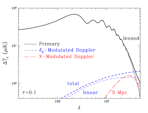
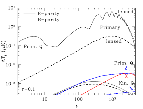
Although we maintain generality in all derivations, we illustrate our results with a $\Lambda$CDM model. The parameters for this model are $\Omega_{c}=0.30$, $\Omega_{b}=0.05$, $\Omega_{\Lambda}=0.65$, $h=0.65$, $Y_{p}=0.24$, $n=1$, and $\delta_{H}=4.2\times 10^{-5}$. This model has mass fluctuations on the $8h$ Mpc^-1 scale in accord with the abundance of galaxy clusters $\sigma_{8}=0.86$. A reasonable value here is important since many of the effects discussed below are nonlinearly dependent on the amplitude of mass fluctuations at or below this scale. We consider reionization redshifts in the range $5\lesssim z_{i}\lesssim 30$ or $0.025\lesssim\tau\lesssim 0.3$. For reference, the primary anisotropies and polarization for a model with $\tau=0.1$ ($z_{i}=13$) is shown in Figs. 1 and 2 respectively

2.2. Secondary Anisotropies

The motion of the scatterers imprints a temperature fluctuation on the CMB through the Doppler effect

$$\Theta(\hat{\bf n})=\int dD\,g(D){\hat{\bf n}}\cdot{\bf v}_{b}({\bf x})\,,$$ (14)

where $\hat{\bf n}$ is the direction on the sky, and ${\bf v}_{b}$ is the velocity field of the baryons and is evaluated along the line of sight ${\bf x}=D\hat{\bf n}$.

Let us first consider the case where the visibility $g$ is dependent on time only. The source ${\hat{\bf n}}\cdot{\bf v}_{b}$ is a field that depends both on direction and on spatial position. It is useful to decompose the Fourier transform of the velocity field into a scalar and two vector (vorticity) modes

$${\bf v}_{b}({\bf k})=-iv_{b}^{(0)}{\bf e}_{3}+\sum_{m=\pm 1}v_{b}^{(m)}{{\bf e}_{2}\mp i{\bf e}_{1}\over\sqrt{2}}\,,$$ (15)

such that

$$\hat{\bf n}\cdot{\bf v}_{b}({\bf k})=-i\sqrt{4\pi\over 3}\sum_{m=-1}^{1}v_{b}^{(m)}Y_{1}^{(m)}(\hat{\bf n})\,,$$ (16)

where ${\bf e}_{3}\parallel\hat{\bf k}$. As shown in the Appendix, the angular power spectrum resulting from the weighted projection of a source with a local dipolar angular dependence is (see equation [A18]),

$$C_{\ell}^{\Theta\Theta}\!\!\! = \!\!\!{\pi^{2}\over\ell^{3}}\int dD\,g^{2}D_{A}\sum_{m=\pm 1}\Delta_{v_{b}}^{2\,(m)}\,,$$ (17)

for $\ell\gg 1$. The power per logarithmic interval in the velocity field $\Delta_{v_{b}}^{2\,(m)}$ is evaluated at the wavenumber that projects onto the angular scale $\ell$ at $D$,

$$k=H_{0}{\ell\over D_{A}}\,.$$ (18)

The implicit assumption here is that the visibility-weighted source $g(D)v_{b}(k,D)$ is slowly-varying across a wavelength of the perturbation.

We will often use the power per logarithmic interval in $\mu$K² or $n$K${}^{2}=(10^{-3}\mu$K)²

$$\Delta T_{\ell}^{2}={\ell(\ell+1)\over 2\pi}C_{\ell}^{\Theta\Theta}T_{\rm CMB}^{2}\,,$$ (19)

where $T_{\rm CMB}=2.728\times 10^{6}$ $\mu$K. The rule of thumb for $\Delta T_{\ell}^{2}$ is that it is of order the logarithmic power spectrum of the source (at cosmological distances $D_{A}\sim 1$) divided by the multipole $\ell$. This factor of $\ell$ comes from the loss of modes parallel to the line of sight due to crest-trough cancellation of the contributions.

Notice however that the $m=0$ potential flow component drops out of the final expression and violates this rule. In a potential flow waves perpendicular to the line of sight lack a velocity component parallel to the line of sight; consequently there is no Doppler effect to leading order (Kaiser 1984). Ostriker & Vishniac (1986) pointed out that the same is not true for vortical flows since waves that run perpendicular to the line of sight have velocities parallel to the line of sight. Since flows in the linear regime are potential, the leading order Doppler effect is nonlinear in the perturbations at small scale.

It is not necessary for the flows themselves to possess vorticity. Since it is the visibility-weighted velocity field $g{\bf v}_{b}$ that is the real source, spatial modulations in the visibility create an effective velocity field

$${\bf v}_{b}(1+\delta g/g)\equiv{\bf v}_{b}+{\bf v}_{g}\,,$$ (20)

which can be used in place of ${\bf v}_{b}$ in equation (17). Spatial variations in the free electron density modulate the visibility and themselves may be caused by fluctuations in the net baryon density (see §3) or the ionization fraction (see §6).

2.3. Secondary Polarization

Thomson scattering of radiation with a quadrupole anisotropy

$$Q^{(m)}({\bf x})=-\int d\Omega\,{Y_{2}^{m*}(\hat{\bf n})\over\sqrt{4\pi}}\Theta({\bf x},\hat{\bf n})$$ (21)

generates linear polarization in the CMB. In terms of the Stokes $q$ and $u$ parameters

$$[q\pm iu](\hat{\bf n})\!\!\! = \!\!\!{\sqrt{24\pi}\over 10}\int dD\,g\sum_{m=-2}^{2}Q^{(m)}{}_{\pm 2}Y_{2}^{m}(\hat{\bf n})\,,$$ (22)

where $Q^{(m)}$ are the 5 quadrupole moments of the temperature fluctuation and ${}_{\pm 2}Y_{\ell}^{m}$ are the spin-2 spherical harmonics (Goldberg et al. 1967).

Some subtleties arises when defining the Fourier transform of the quadrupole source since the orientation of the coordinate system enters into its definition. It is convenient to chose the reference frame so that $\hat{\bf e}_{3}\parallel{\bf k}$, and this choice will be understood unless otherwise specified. The consequence is an ambiguity in combining contributions from different ${k}$-modes but these can be removed by defining the coordinate independent components of the polarization (Zaldarriaga & Seljak 1997; Kamionkowski et al. 1997),

$$[q\pm iu](\hat{\bf n})\!\!\! = \!\!\!\sum_{\ell}\sum_{m=-2}^{2}[E_{\ell}^{(m)}\pm iB_{\ell}^{(m)}]{}_{\pm 2}Y_{2}^{m}(\hat{\bf n})\,.$$ (23)

Since polarization is a spin-2 field and its source has a local quadrupole angular dependence, its power spectrum is given by equation (A18) with $s=\pm 2$ and $j=2$. The power spectra of the $E$ and $B$ parity states are then

$$C_{\ell}^{EE}\!\!\! = \!\!\!{3\pi^{2}\over 10\ell^{3}}\int dD\,g^{2}D_{A}\left({3\over 4}\Delta_{Q}^{2\,(0)}+{1\over 8}\sum_{m=\pm 2}\Delta_{Q}^{2\,(m)}\right)\,,$$

$$C_{\ell}^{BB}\!\!\! = \!\!\!{3\pi^{2}\over 10\ell^{3}}\int dD\,g^{2}D_{A}{1\over 2}\sum_{m=\pm 1}\Delta_{Q}^{2\,(m)}\,,$$ (24)

again evaluated with the projection equation (18) and a slowly-varying source. We define the logarithmic power spectrum of the polarization in the same way as for the anisotropies (see equation [19]). It is likewise down by a factor of $\ell$ from the power spectrum of the source except when the angular dependence of the source reduces it further as in the case of $B$-parity polarization from $m=0,\pm 2$ and $E$-parity polarization from $m=\pm 1$.

As pointed out by Kaiser (1984) and examined quantitatively by Efstathiou (1988), the polarization, even more than the temperature anisotropy, is suppressed by cancellation at small scales. The reason is simply that the source of the polarization is the temperature anisotropy (quadrupole moment) and thus both the source and its contributions along the line of sight are suppressed.

The dominant source at small angles is again the visibility modulation of the large scale quadrupole anisotropy

$$Q^{(m)}\rightarrow Q^{(m)}(1+\delta g/g)\equiv Q^{(m)}+Q_{g}^{(m)}\,.$$ (25)

We will consider quadrupole sources $Q^{(m)}$ in §4, the effect of density modulation in §5, and that of ionization modulation in §6.

3. Density-Modulated Anisotropies

In this section we consider the temperature anisotropies that arise from the modulation of the Doppler effect due to density inhomogeneities. We begin with a review of the second-order effect from linear density fluctuations (§3.1) and then generalize the calculation to include small-scale nonlinearities in the density field (§3.2).

3.1. Linear Fluctuations: Vishniac Effect

Spatial variations in the opacity due to density perturbations in the baryons modulates the visibility: $\delta g/g=\delta_{b}$. When $\delta_{b}$ is in the linear regime, the result is called the Vishniac (1987) effect. In this section, we rederive the Vishniac effect in a manner that will make its nonlinear generalization obvious.

The Fourier transform of ${\bf v}_{g}$ is a convolution of the linear velocity and density fields,

$${\bf v}_{g}({\bf k})=\int{d^{3}k_{1}\over(2\pi)^{3}}{\bf v}_{b}({\bf k}_{1})\delta_{b}(k_{2})\,,$$ (26)

where here and througout

$${\bf k}_{2}={\bf k}-{\bf k}_{1}\,.$$ (27)

The two vortical components to the velocity field are given by the projections (see equation [15])

$$v_{g}^{(\pm 1)}({\bf k})\!\!\! = \!\!\!{\hat{\bf e}_{2}\pm i\hat{\bf e}_{1}\over\sqrt{2}}\cdot{\bf v}_{g}\,,$$

$$= \!\!\!\sqrt{4\pi\over 3}\int{d^{3}k_{1}\over(2\pi)^{3}}v_{b}(k_{1})\delta_{b}(k_{2})Y_{1}^{\pm 1*}(\hat{\bf k}_{1})\,,$$

in the basis where ${\bf e}_{3}\parallel{\bf k}$. We have assumed that the underlying velocity field is a potential flow ${\bf v}_{b}({\bf k})=-iv_{b}(k)\hat{\bf k}$.

The power spectrum then becomes

$$\Delta_{v_{g}}^{2\,(1)}={1\over 3}\int{dk_{1}\over k_{1}}d\Omega\,{k^{3}\over k_{2}^{3}}|Y_{1}^{1}({\bf k}_{1})|^{2}[A+B]\,,$$ (29)

and likewise for the $m=-1$ component. The two contributions are from the velocity-velocity, density-density power spectra

$$A=\Delta^{2}_{v_{b}}(k_{1})\Delta^{2}_{\delta_{b}}(k_{2})\,,$$ (30)

and the velocity-density cross correlation power spectra

$$B=-{k_{1}\over k_{2}}\Delta^{2}_{v_{b}\delta_{b}}(k_{1})\Delta^{2}_{v_{b}\delta_{b}}(k_{2})\,,$$ (31)

where we have used the relation

$$Y_{1}^{1}({\bf k}_{2})=-{k_{1}\over k_{2}}Y_{1}^{1}({\bf k}_{1})\,.$$ (32)

Substituting equation (29) and (17) after reexpressing the velocity power spectrum with the density power spectrum using equation (9), we obtain

$$C_{\ell}^{\Theta\Theta}\!\!\! = \!\!\!{\pi^{2}\over 2\ell^{5}}\int{dD}\,D_{A}^{3}\left(g{\dot{G}\over G}\right)^{2}\Delta_{\delta_{b}}^{4}I_{V}\,,$$ (33)

where we have used the fact that $m=\pm 1$ contributes equally. The mode coupling integral is

$$I_{V}\!\!\! = \!\!\!\int_{0}^{\infty}dy_{1}\int_{-1}^{1}d\mu{(1-\mu^{2})(1-2\mu y_{1})\over y_{1}^{3}y_{2}^{5}}{\Delta^{2}_{\delta_{b}}(ky_{1})\over\Delta^{2}_{\delta_{b}}(k)}{\Delta^{2}_{\delta_{b}}(ky_{2})\over\Delta^{2}_{\delta_{b}}(k)}\,.$$

Here and throughout

$$\mu\!\!\! = \!\!\!\hat{\bf k}\cdot\hat{\bf k}_{1}\,,$$

$$y_{1}\!\!\! = \!\!\!k_{1}/k\,,$$

$$y_{2}\!\!\! = \!\!\!k_{2}/k=\sqrt{1-2\mu y_{1}+y_{1}^{2}}\,.$$ (35)

The form of the mode coupling integral in equation (LABEL:eqn:modecoupling) is 1/2 that of Vishniac (1987) equation (2.13), which resolves the apparent discrepancy with Dodelson & Jubas (1995) raised by Jaffe & Kamionkowski (1998). As pointed out by Dodelson & Jubas (1995), this form is easier to evaluate numerically. Additionally, for our purposes, it better brings out the small-scale limit.

Figure 3.— Velocity-density decoupling and density nonlinearities. For the fiducial $\Lambda$CDM model the velocity and density fields decorrelate in the Vishniac calculation ($I_{V}^{\rm dec}/I_{V}\approx 1$) before the onset of nonlinearity in the density field, especially at high redshift where most of the scattering occurs.

For wavelengths that are much smaller than the coherence scale of the velocity field, these expressions simplify considerably. The density-velocity cross correlation (31) vanishes and the remaining term (30) can be evaluated under the approximation $k_{2}=|{\bf k}-{\bf k}_{1}|\approx k$,

$$\Delta_{v_{g}}^{2\,(\pm 1)}={1\over 3}\Delta^{2}_{\delta_{b}}v_{\rm rms}^{2}\,,$$ (36)

where we have used the orthogonality of spherical harmonics $\int d\Omega\,Y_{\ell}^{m*}Y_{\ell^{\prime}}^{m^{\prime}}=\delta_{\ell,\ell^{\prime}}\delta_{m,m^{\prime}}$ and

$$v_{\rm rms}^{2}=\int{dk\over k}\Delta_{v_{b}}^{2}\,.$$ (37)

Note that $v_{\rm rms}^{2}$ is still a function of $D$.

Equation (38) has a simple interpretation. At small scales, the effect arises from a density modulation of a uniform bulk velocity from larger scales whose rms in each component is 1/3 of the total.

Substituting the velocity power spectrum relation (36) into equation (29) yields

$$C_{\ell}^{\Theta\Theta}\!\!\! = \!\!\!{2\pi^{2}\over 3\ell^{3}}\int{dD}\,D_{A}g^{2}\Delta_{\delta_{b}}^{2}v_{\rm rms}^{2}\,.$$ (38)

This equation may alternately be derived from equation (33) in the limit that the integral gets its contribution from $y_{1}\ll 1$,

$$I_{V}^{\rm(dec)}\!\!\! = \!\!\!{4\over 3}\int_{0}^{\infty}{dy_{1}\over y_{1}^{3}}{\Delta^{2}_{\delta_{b}}(ky_{1},\eta)\over\Delta^{2}_{\delta_{b}}(k,\eta)}\,,$$ (39)

$$= \!\!\!{4\over 3}\left({G\over\dot{G}}{k\over H_{0}}\right)^{2}{v_{\rm rms}^{2}\over\Delta^{2}_{\delta_{b}}}$$

In Fig. 3, we show that for the $\Lambda$CDM model, the density and velocity contributions decouple in this manner beyond $k\sim 0.2h$Mpc^-1. The approximation (39) represents an efficient way of evaluating the otherwise computationally expensive the mode coupling integral in this regime.

3.2. Nonlinear Perturbations: Kinetic SZ Effect

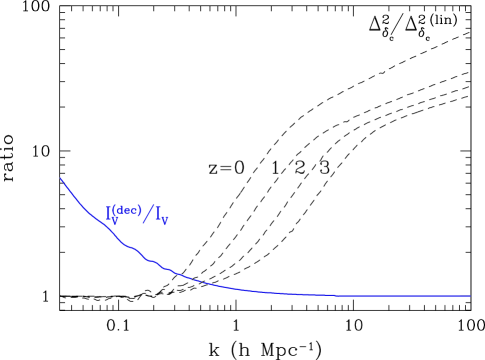
Nonlinear density fluctuations caught up in a bulk flow from larger scales gives rise to the kinetic Sunyaev-Zel’dovich effect from large-scale structure. It can alternately be thought of as the nonlinear extension of the Vishniac effect. The reason is that in adiabatic CDM cosmologies nonlinearities only affect the density field below the coherence scale of the bulk velocity. Recall that in this limit the Vishniac effect arises from density perturbations caught in a large-scale flow to which it is uncorrelated.

Figure 3 illustrates this fact for the fiducial $\Lambda$CDM. Notice that even at $z=0$, the dark matter density field only deviates substantially from the linear approximation after equation (39) becomes a good description of the Vishniac effect. If we then replace the linear density power spectrum with its nonlinear analogue but leave the contribution from the velocity power spectrum the same, we obtain

$$C_{\ell}^{\Theta\Theta}\!\!\! = \!\!\!{\pi^{2}\over 2\ell^{5}}\int{dD}\,D_{A}^{3}\left(g{\dot{G}\over G}\right)^{2}\Delta^{2\,({\rm lin})}_{\delta_{b}}\Delta^{2}_{\delta_{b}}I_{V}\,,$$ (40)

with the mode coupling integral $I_{V}$ using equation (LABEL:eqn:modecoupling) evaluated under linear theory. This expression has the nice feature that it expresses the total effect: it includes both the Vishniac effect and the kinetic SZ effect from nonlinear structures.

The underlying assumption is that the density fluctuations in the nonlinear regime are uncorrelated with the bulk velocity field. Nonlinear evolution in the density field will correlate velocity and density modes if they are both in the nonlinear regime. However, the bulk flow in adiabatic CDM models arises mainly from the linear regime. In the $\Lambda$CDM model, half the contributions to $v_{\rm rms}^{2}$ comes from scales $k<0.07h$Mpc^-1 and the fluctuations go nonlinear at $k\sim 0.2h$Mpc^-1. Scoccimarro et al. (1999) found that for the 4-point statistics, nonlinear modes are highly correlated but that the correlation drops rapidly as one pair of the modes enters the linear regime. Decorrelation is even more effective here since the relevant velocity and density modes are oriented perpendicular to each other.

Once the nonlinear power spectrum of the baryonic gas is known, the resultant anisotropies can be calculated with equation (40). This unfortunately requires hydrodynamic simulations in general and ab initio attempts in the literature (e.g. Persi et al.  1995) to simulate the scattering effects have not had the dynamic range to treat the full problem. Let us instead break the problem into two: calculate the effect under the assumption that the gas tracks the dark matter and then estimate where this approximation may break down.

Figure 4.— Nonlinear vs. linear power spectra for the CDM under the Peacock & Dodds (1996) scaling approximation and for the baryons under the additional prefiltering ansatz of Gnedin & Hui (1998). Note that the dilation of scales brings the filtering scale deep into the nonlinear regime.

3.2.1 Maximal Effect

Let us first consider the effect under the simple assumption that the gas traces the dark matter to place an upper limit on the magnitude of the effect. The nonlinear dark matter power spectrum has been well-studied with N-body simulations for the full range of adiabatic CDM cosmologies. Hamilton et al. (1991) suggested a useful scaling relation for the correlation function in the nonlinear regime that was generalized to the power spectrum by Peacock & Dodds (1994). The underlying idea is that nonlinear fluctuations on a scale $k$ arise from linear fluctuations on a larger scale

$$k_{\rm lin}=[1+\Delta_{\delta_{c}}^{2}(k)]^{-1/3}k\,,$$ (41)

so that there is a functional relation between the nonlinear and linear power spectra at these two scales

$$\Delta_{\delta_{c}}^{2}(k)=f_{\rm NL}[\Delta_{\delta_{c}}^{2\,{\rm(lin)}}(k_{\rm lin})]\,,$$ (42)

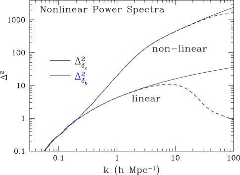
which may be fit to simulations. We take the Peacock & Dodds (1996; eqn. [21]-[27]) form for $f_{\rm NL}$. The resulting power spectrum for the $\Lambda$CDM model are shown in Fig. 4.

Figure 5.— Maximal nonlinear enhancement of the Vishniac effect. Under the assumption that the gas density traces the dark matter density into the deeply nonlinear regime the Vishniac effect is significantly enhanced by nonlinearities at $\ell\gtrsim 1000$ especially in the late reionization scenarios.

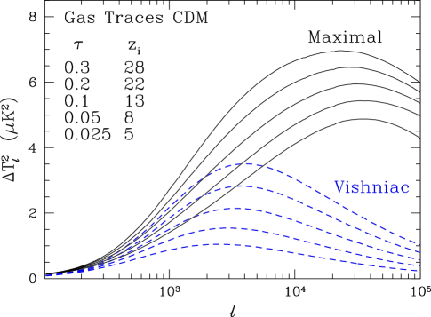
Under this assumption, the kinetic SZ effect provides a significant enhancement of the Vishniac effect. As shown in Fig. 5, the relative contribution is the largest for late reionization scenarios (low $z_{i}$) because anisotropies then arise from structure that is well-developed. However one must keep in mind that this is essentially an upper limit to the contributions since the gas pressure will smooth out the gas density below the Jeans scale.

Figure 6.— Prefiltering the dark matter spectrum. Prefiltering the power spectrum to account for gas pressure as in Fig. 4 cuts off the anisotropies at $\ell\sim 10^{4}$ for the $\Lambda$CDM model.

3.2.2 Pressure Cutoff

Gnedin & Hui (1998) examined simple schemes to approximate the effect of gas pressure. One such scheme that has fractional errors on the 10% level for overdensities $\lesssim 10$ is to filter the density perturbations in the linear regime as $\Delta_{\delta_{b}}^{2}=f_{b}^{2}(k/k_{\rm F})\Delta_{\delta_{c}}^{2}$ and treat the system as collisionless baryonic particles. Their best fit is obtained with the filter

$$f_{b}={1\over 2}[e^{-x^{2}}+{1\over(1+4x^{2})^{1/4}}]$$ (43)

and Gnedin (1998) suggests $k_{\rm F}=34\Omega_{m}^{1/2}h$Mpc^-1 as a reasonable choice for the thermal history dependent filtering scale.

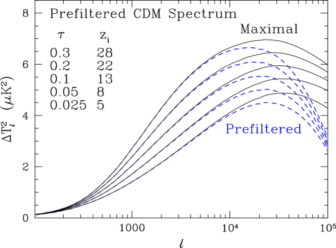
The results of applying the nonlinear scaling relation of equation (42) to the filtered linear power spectrum are shown in Fig. 4. Notice that the dilation in wavenumber takes the filtering scale deep into the nonlinear regime. The calculations should not be trusted beyond this scale since the nonlinear scaling breaks down for spectra with a sharp cut off; indeed we have taken the local slope of the unfiltered spectrum rather than the filtered spectrum when evaluating the Peacock & Dodds (1996) formulae. Still the result displayed in Fig. 6 imply that the gas-traces-CDM assumption is reasonable in the arcminute regime $\ell\lesssim 10^{4}$.

Figure 7.— Postfiltering the dark matter spectrum. Filtering the CDM power spectrum with equation (44) introduces a smooth cut off at small angles and shows that nonlinearities are important as long as the gas traces the dark matter out to $\Delta_{F}\sim 10$.

To give a more model-independent quantification of this effect, let us also consider a baryonic power spectrum given by

$$\Delta_{\delta_{b}}^{2}(k)=\Delta_{\delta_{c}}^{2}(k)\exp(-\Delta_{\delta_{c}}^{2}/\Delta_{F}^{2})\,.$$ (44)

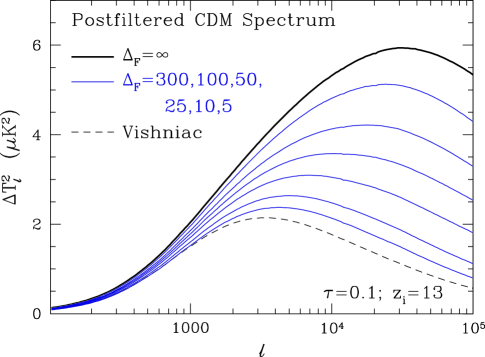
The results for several values of $\Delta_{F}$ are given in Fig. 7 and show that only if the baryons fail to trace the dark matter out to $\Delta_{F}\sim 10$ can nonlinear effects be ignored.

Our analysis shows that the kinetic SZ effect should be an important contributor to small-angle anisotropies. On arcminute scales and above, the assumption that the gas traces the dark matter is reasonable given our current understanding of the thermal history of adiabatic CDM models. The amplitude of the effect at the subarcminute scales will depend on the details of thermal history throughits effect on the clustering of the gas. Observations in this regime may open a new window on the physics of this regime. Isolation of this effect from foregrounds (e.g. radio and infrared point sources) and other secondary anisotropies (e.g. the inhomogeneous reionization signal considered in §6) will be the main obstacle to overcome.

Figure 8.— The power spectrum of the present-day quadrupole from the projection of primordial temperature inhomogeneities and the kinematic Doppler effect in the $\Lambda$CDM model. The primordial quadrupole has been calculated numerically with a Boltzmann code.

4. Polarization from Homogeneous Scattering

In this section we consider the origin of quadrupole anisotropies and the linear polarization they generate through Thomson scattering in a homogeneous medium. The quadrupole anisotropies fall into three broad classes: the primordial quadrupole from the projection of Sachs-Wolfe temperature anisotropies, the intrinsic quadrupole from scattering (§4.1), and the kinematic quadrupole from the second order Doppler effect (§4.2).

4.1. Primordial and Intrinsic Quadrupoles

A large-scale temperature inhomogeneity at the recombination epoch ($z\sim 10^{3}$) from the Sachs-Wolfe gravitational redshift effect $\Theta=-\Phi/3$ becomes a quadrupole anisotropy at low redshifts by simple projection. In other words, the spherical harmonic decomposition of the plane wave fluctuation,

$$-{\Phi\over 3}\exp(i{\bf k}\cdot{\bf x})\rightarrow-{\Phi\over 3}j_{\ell}({k\over H_{0}}D)Y_{\ell}^{0}\,,$$ (45)

yields a spectrum of anisotropies and in particular a quadrupole anisotropy given by

$$Q^{(0)}=-\sqrt{5}{\Phi\over 3}j_{2}({k\over H_{0}}D_{*})\,.$$ (46)

Here $D_{*}=D_{\rm rec}-D$ and we have assumed that spatial curvature can be neglected at reionization. Curvature corrections may be included by replacing the spherical bessel function $j_{2}$ with the hyperspherical bessel function $\Phi_{2}^{\nu}$ (see Appendix).

The logarithmic power spectrum of the quadrupole can therefore be expressed in terms of that of the potential as

$$\Delta_{Q}^{2\,(0)}\!\!\! = \!\!\!{5\over 9}j_{2}^{2}({k\over H_{0}}D_{*})\Delta_{\Phi}^{2}$$ (47)

$$= \!\!\!{5\over 4}\delta_{H}^{2}\left({k\over H_{0}}\right)^{n-1}(1+z)^{2}G^{2}\Omega_{m}^{2}j_{2}^{2}({k\over H_{0}}D_{*})\,,$$

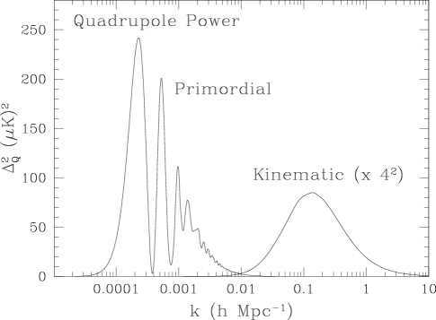
where the second line employs equation (7) and again assumes matter domination at $D$. We show the results of numerically calculating the quadrupole power spectrum from a cosmological Boltzmann code (White & Scott 1996) in Fig. 8. Note that the spectrum peaks at large scales, corresponding to the horizon at the reionization epoch $k\sim H_{0}/D_{*}$. On smaller scales, the projection (45) carries the power to higher angular moments.

The rms is the integral over the power spectrum

$$Q_{\rm rms}^{2}\!\!\! = \!\!\!\int{dk\over k}\Delta_{Q}^{2\,(0)}\,,$$ (48)

$$= \!\!\!{5\over 4}\delta_{H}^{2}(1+z)^{2}G^{2}\Omega_{m}^{2}(D_{*}H_{0})^{1-n}\int dxx^{n}j_{2}^{2}(x)\,,$$

$$= \!\!\!{5\over 48}\delta_{H}^{2}(1+z)^{2}G^{2}\Omega_{m}^{2}(D_{*}H_{0})^{1-n}\Gamma_{\rm SW}(n)\,,$$

where

$$\Gamma_{\rm SW}(n)=3\sqrt{\pi}{\Gamma[(3-n)/2]\over\Gamma[(4-n)/2]}{\Gamma[(3+n)/2]\over\Gamma[(9-n)/2]}\,.$$ (49)

For reference, note that $Q_{\rm rms}^{2}=5C_{2}^{\Theta\Theta}/4\pi$. For our fiducial $\Lambda$CDM model $\delta_{H}=4.2\times 10^{-5}$, $(1+z)G=1.24$, and $\Gamma_{\rm SW}(1)=1$, we obtain $Q_{\rm rms}T_{\rm CMB}=16\mu$K.

There are two effects that modify this result slightly. The first is that the universe may not be completely matter-dominated at the time of scattering. Additional anisotropies are then created as the gravitational potential decays. At high redshifts, the effect of the radiation energy density pushes the quadrupole anisotropy up via the “early” integrated Sachs-Wolfe effect (Hu & Sugiyama 1995); correspondingly at low redshifts the effect of the cosmological constant or curvature again pushes the quadrupole up via the “late” integrated Sachs-Wolfe effect (Kofman & Starobinskii 1985). These effects are clearly visible in Fig. 10, where we plot the evolution of the rms quadrupole from numerical calculations.

The second effect is that scattering itself can produce quadrupole anisotropies through projection of the Doppler effect and also destroy the primordial quadrupole through isotropization. We call the net effect the contributions of the intrinsic quadrupole. This effect is suppressed both by the assumed optically thin conditions and by the fact that the Doppler effect is cancelled except on scales near the horizon where the velocity itself is small. In Fig. 10, this effect is barely visible as a blip near the redshift of reionization.

The hallmark of all these effects is that they create only $m=0$ type quadrupoles, because they come from ($\ell=0$, $m=0$) gravitational potential perturbations and ($\ell=1$, $m=0$) potential flows. They therefore generate only $E$-parity polarization. The polarization from these sources are not slowly varying across a wavelength of the horizon-sized perturbations and hence the approximation developed in the Appendix cannot be used to calculate these effects. They are however automatically included in cosmological Boltzmann codes. We show the resulting polarization in Fig. 2 for the $\Lambda$CDM model as calculated with CMBFast. As is well known, the secondary polarization from these effects are confined to the lowest $\ell$ since the quadrupole sources contribute mainly on horizon scales at last scattering.

4.2. Kinematic Quadrupole

As pointed out by Sunyaev & Zel’dovich (1980), in the rest frame of the scatterers, an isotropic CMB gains a quadrupole anisotropy from the quadratic Doppler effect

$$\Theta={\sqrt{1-v_{b}^{2}}\over 1-\hat{\bf n}\cdot{\bf v}_{b}}-1\approx\hat{\bf n}\cdot{\bf v}_{b}+(\hat{\bf n}\cdot{\bf v}_{b})^{2}-{1\over 2}v_{b}^{2}\,,$$ (50)

that induces a polarization in the CMB by Thomson scattering. In real space, the quadrupole moment is simply

$$Q^{(0)}({\bf x})={2\over 3\sqrt{5}}v_{b}^{2}({\bf x})$$ (51)

in the basis aligned with the velocity $\hat{\bf e}_{3}\parallel{\bf v}_{b}({\bf x})$; in Fourier space with a basis $\hat{\bf e}_{3}\parallel\hat{\bf k}$, the expression is more involved

$$Q^{(m)}\!\!\! = \!\!\!-\int d\Omega\,{Y_{2}^{m*}(\hat{\bf n})\over\sqrt{4\pi}}\int{d^{3}k_{1}\over(2\pi)^{3}}\hat{\bf n}\cdot{\bf v}_{b}({\bf k}_{1})\,\hat{\bf n}\cdot{\bf v}_{b}({\bf k}_{2})$$ (52)

$$= \!\!\!-{2\sqrt{4\pi}\over 15}\int{d^{3}k_{1}\over(2\pi)^{3}}v_{b}(k_{1})v_{b}(k_{2}){k_{1}\over k_{2}}$$

$$\!\!\!\quad\times\left[Y_{2}^{m*}(\hat{\bf k}_{1})-\sqrt{5\over 3+|m|}{k\over k_{1}}Y_{1}^{m*}(\hat{\bf k}_{1})\right]\,,$$

where $Y_{1}^{2}=Y_{1}^{-2}=0$. The logarithmic power spectrum becomes

$$\Delta_{Q}^{2\,(m)}={4\over 45}\Delta_{v_{b}}^{2}(k)\Delta_{v_{b}}^{2}(k)I_{Q}^{(m)}\,,$$ (53)

where the mode coupling integrals are given by

$$I_{Q}^{(m)}\!\!\! = \!\!\!\int_{0}^{\infty}dy_{1}\int_{-1}^{1}d\mu{a^{(m)}\over y_{1}y_{2}^{3}}{\Delta_{v_{b}}^{2}(ky_{1})\over\Delta_{v_{b}}^{2}(k)}{\Delta_{v_{b}}^{2}(ky_{2})\over\Delta_{v_{b}}^{2}(k)}\,.$$ (54)

Here the angular arguments are

$$a^{(\pm 2)}\!\!\! = \!\!\!{3\over 8}y_{1}^{2}(1-\mu^{2})^{2}\,,$$

$$a^{(\pm 1)}\!\!\! = \!\!\!{3\over 8}(1-2\mu y_{1})^{2}(1-\mu^{2})\,,$$

$$a^{(0)}\!\!\! = \!\!\!{1\over 4}[2\mu-y_{1}(3\mu^{2}-1)]^{2}\,,$$ (55)

and it is useful to define the auxilary quantity

$$a^{(f)}={1\over 4}(1-\mu^{2})\,.$$ (56)

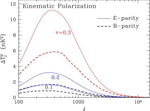
The polarization power spectrum then follows by inserting equation (53) in equation (24). The result for the $\Lambda$CDM cosmology is shown in Fig. 9

Figure 9.— Power spectra of $E$- and $B$-parity polarization from the kinematic quadrupole in the $\Lambda$CDM model.

The rms quadrupole follows simply from the relation

$$\sum_{m=-2}^{2}a^{(m)}=y_{2}^{2}-a^{(f)}$$ (57)

with a change of variables to ${\bf k}_{2}$ for the integration of the first term

$$Q_{\rm rms}^{2}\!\!\! = \!\!\!\int{dk\over k}\sum_{m=-2}^{2}\Delta_{Q}^{2\,(m)}={8\over 45}(1-f_{\rm kin})v_{\rm rms}^{4}$$ (58)

$$f_{\rm kin}\!\!\! = \!\!\!{1\over 2}\int{dk\over k}{\Delta_{v_{b}}^{2}\Delta_{v_{b}}^{2}\over v_{\rm rms}^{4}}I_{Q}^{(f)}\,.$$

For the $\Lambda$CDM model $f_{\rm kin}=0.16$. This expression is smaller than the naive expectation implied by real space relation (51), $4\left<v_{b}^{4}\right>/45=12v_{\rm rms}^{4}/45$, because the quadrupole is oriented and not simply a scalar gaussian random field. The main effect can be understood as the contribution from the variance of $v_{b}^{2}$, $\left<v_{b}^{4}\right>-\left<v_{b}^{2}\right>^{2}=2v_{\rm rms}^{4}$, since its mean value comes from contributions that cancel out in orientation for the quadrupole.

Figure 10.— The time evolution of the rms quadrupole in the $\Lambda$CDM model. Upper curves: the various linear theory effects (see text) for three different ionization histories from numerical calculations. Lower curves: the kinematic effect.

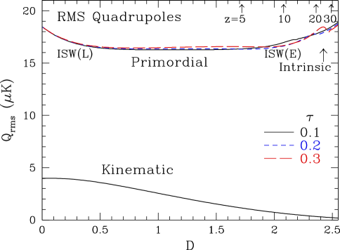
The kinematic quadrupole is not negligible in comparison with the primordial quadrupole for $\Lambda$CDM or indeed any model that fits the observations. Large angle anisotropies are observed today at $10^{-5}$ while the velocity field reaches $10^{-3}$. As shown in Fig. 10, for $\Lambda$CDM it is approximately $1/4$ the primordial one in amplitude today. Furthermore, equation (53) implies that it generates comparable power in all 5 $m$-modes of the quadrupole and hence comparable $E$ and $B$ parity polarization. One might naively assume that the kinematic effect generates as much $B$-parity polarization as the primordial quadrupole generates $E$. This would then be an obstacle for detecting gravity waves through the $B$-parity polarization.

There are however two reasons why the polarization is much smaller than implied by these arguments. The first is that the $v_{\rm rms}^{2}$ declines as $(1+z)^{-1}$ in the matter-dominated epoch whereas the primordial quadrupole remains constant. The second is that in the $\Lambda$CDM model the coherence of the velocity field is over 2 orders of magnitude smaller than that of the primordial quadrupole and hence generates polarization at $\ell\sim 400$. Recall that the rule of thumb for projected sources is that the angular power spectrum is down by one factor of $\ell$ from the spatial power spectrum. This produces another order of magnitude suppression of the polarization (see Fig. 9). The $B$-parity polarization generated here is significantly smaller than that generated by gravitational lensing of the primary polarization (Zaldarriaga & Seljak 1998). This effect is therefore unlikely to be detectable in $\Lambda$CDM models.

It is worth emphasizing that the amplitude of this effect is highly model dependent and scales in power as $v_{\rm rms}^{4}\lambda_{v}$ where $\lambda_{v}$ is the coherence scale of the velocity field. Upper limits on the $B$-polarization can therefore constrain the amplitude and coherence of the velocity field. For example consider a velocity field with an rms of $\sim 700$km s^-1 on the a tophat scale of 150$h^{-1}$ Mpc is suggested by the data of Lauer & Postman (1994). If we model that field by the $\Lambda$CDM velocity power spectrum but increase the coherence length by a factor of 10 and the rms velocity by 1.55, we boost the polarization power by $1.55^{4}\times 10=58$ and angular scale by 10 ($\ell\sim 40$). The power would be even larger in an open universe where the velocity amplitude actually grows substantially with redshift before declining. It is also worth bearing in mind that effects such as these warn against blindly taking even a large-angle detection of $B$-polarization as a model-independent detection of gravity waves or vorticity.

Finally, note that the correlation between primary and secondary temperature anisotropies and the kinematic polarization is suppressed since it involves the three-point function of the density field and hence vanishes in the linear regime.

5. Density-Modulated Polarization

Here we consider the polarization generated from the density-modulation of the quadrupole anisotropies considered in the last section. Again these are separated by the nature of the quadrupole source: the primordial quadrupole §5.1, the kinematic quadrupole §5.2, and the intrinsic quadrupole §5.3.

5.1. Primordial Quadrupole

For the modulation of the primordial quadrupole by density fluctuations, we have

$$Q^{(m)}_{g}(k)=\int{d^{3}k_{1}\over(2\pi)^{3}}Q^{(m)}({\bf k}_{1})\delta_{b}(k_{2})\,,$$ (59)

Scalar perturbations in linear theory only generate $m=0$ quadrupoles in the ${\bf k}_{1}$-basis, i.e. $Q^{(0)}(k_{1})Y_{2}^{0}(\beta,\alpha)$ where $\beta$ and $\alpha$ are the polar and azimuthal angles defining $\hat{n}$ in this basis. One can project this onto the ${\bf e}_{3}\parallel{\bf k}$ basis with the help of the angular addition relation (see Hu & White 1997 eq. [7]),

$$Y_{2}^{0}(\beta,\alpha)=\sqrt{4\pi\over 5}\sum_{m}Y_{2}^{m*}({\bf k}_{1})Y_{2}^{m}(\hat{\bf n})$$ (60)

such that

$$Q^{(m)}_{g}(k)=\sqrt{4\pi\over 5}\int{d^{3}k_{1}\over(2\pi)^{3}}Q^{(0)}(k_{1})Y_{2}^{m*}(\hat{\bf k}_{1})\delta_{b}(k_{2})\,,$$ (61)

Since the quadrupole source $Q^{(0)}(k_{1})$ peaks on the scale of the horizon whereas the density perturbations rise to small scales in adiabatic CDM models, the correlation decouples

$$\Delta_{Q_{g}}^{2\,(m)}={1\over 5}\Delta_{\delta_{b}}^{2}Q^{2}_{\rm rms}\,,$$ (62)

where we have again used the orthogonality of spherical harmonics and $Q^{2}_{\rm rms}$ is taken from numerical calculations as in Fig. 10. Inserting equation (62) into equation (24), we obtain

$$C_{\ell}^{EE}=C_{\ell}^{BB}={3\pi^{2}\over 50\ell^{3}}\int dD\,D_{A}g^{2}\Delta_{\delta_{b}}^{2}Q_{\rm rms}^{2}\,.$$ (63)

As shown in Fig. 11, even for the gas-traces-CDM assumption the polarization generated by this effect in a $\Lambda$CDM model is small, much smaller than the polarization generated by lensing (cf. Fig. 2).

The cross correlation between multipole moments of the Vishniac effect and the polarization $C_{\ell}^{\Theta E}$ vanishes when averaged over the sky due to the different angular dependence of the underlying dipole and quadrupole sources. Mathematically, this can be seen in the sources (61) and (3.1); the orthogonality of the spherical harmonics guarantees that these terms will integrate to zero when summing over the directions of each $k$-mode.

Note however that there will be a strong correlation between the amplitude of the polarization and the amplitude of the temperature fluctuations and may provide a means of pulling out the signal in models where it is somewhat stronger.

Figure 11.— Density-modulated polarization in each parity type $E=B$ for the $\Lambda$CDM model. Here we assume that the gas traces the dark matter.

5.2. Kinematic Quadrupole

The kinematic quadrupole is also modulated by the density field. Its effect is identical to the primordial quadrupole except equation (58) for the kinetic quadrupole is used in equation (63),

$$C_{\ell}^{EE}=C_{\ell}^{BB}={4\pi^{2}\over 375\ell^{3}}\int dD\,g^{2}D_{A}\Delta_{\delta_{b}}^{2}(1-f_{\rm kin})v_{\rm rms}^{4}\,,$$ (64)

where recall that $f_{\rm kin}$ is a small correction due to the directionality of the quadrupole moments. The ratio integrands between the modulated Doppler and cosmic polarizations is

$${8\over 45}(1-f_{\rm kin}){v^{4}_{\rm rms}\over Q_{\rm rms}^{2}}\,,$$ (65)

Since observationally $v_{\rm rms}\sim(1+z)^{-1/2}10^{-3}$ and $Q_{\rm rms}\sim 10^{-5}$, the effect from the primordial quadrupole is typically larger. We show the results for the fiducial $\Lambda$CDM model in Fig. 2.

5.3. Intrinsic Quadrupole

The quadrupole anisotropy generated by the Vishniac effect during reionization produces a linear polarization intrinsic to the Vishniac effect. This effect is doubly suppressed by cancellation: both the source of the quadrupole and its polarization contributions along the line of sight cancel when integrating along the line of sight.

The quadrupole moment generated by the Vishniac effect is given by equation (A6)

$$Q^{(m)}\!\!\! = \!\!\!\sqrt{5}\int dD\,g(D)v_{g}^{(m)}\alpha_{01,2}^{(m)}$$ (66)

$$\approx \!\!\!\sqrt{3\pi^{2}\over 20}{H_{0}\over k}X\tau_{H}(1+z)^{2}v_{g}^{(m)}\,,$$

and thus the power per logarithmic interval

$$\Delta_{Q}^{2\,(m)}\!\!\! = \!\!\!{3\pi^{2}\over 20}\left({H_{0}\over k}\right)^{2}X^{2}\tau_{H}^{2}(1+z)^{4}\Delta_{v_{g}}^{2\,(m)}\,.$$ (67)

The polarization power spectrum becomes

$$C_{\ell}^{BB}\!\!\! = \!\!\!{9\pi^{4}\over 800\ell^{7}}\int dD\,D_{A}^{5}X^{2}\tau_{H}^{2}(1+z)^{4}\left(g{\dot{G}\over G}\right)^{2}$$ (68)

$$\!\!\!\quad\times\Delta_{\delta_{b}}^{2\,{\rm(lin)}}\Delta_{\delta_{b}}^{2}I_{V}\,,$$

with $C_{\ell}^{EE}=0$ since only $m=\pm 1$ contributes to the Vishniac effect. The integrand in this equation is down by a factor of

$${9\pi^{2}\over 400\ell^{2}}D_{A}^{2}X^{2}\tau_{H}^{2}(1+z)^{4}={\cal O}\left[{\tau^{2}\over\ell^{2}}(1+z)\right]\,,$$ (69)

compared with the temperature anisotropies and is thus highly suppressed at high $\ell\sim 10^{3}$ from an amplitude that is already reduced by the low optical depth $\tau\lesssim 10^{-1}$ in the reionized universe. Finally, there is no cross correlation between the temperature and intrinsic polarization since the polarization is purely of $B$-parity.

Figure 12.— Ionization-modulation effect. A patch size of $5$Mpc and duration of patchiness of $\delta z_{i}/(1+z_{i})=0.25$ in the $\Lambda$CDM model is assumed.

6. Patchy Reionization

Inhomogeneities in the ionization fraction create a modulated Doppler anisotropies and polarization of the CMB just as inhomogeneities in the density. The techniques used in the calculation of density-modulated effects thus can be carried over to here with little modification.

For the modulated doppler effect, one takes ${\bf v}_{g}$ of equation (20) to be ${\bf v}_{b}\delta_{X}$ where $\delta_{X}$ is the fluctuation in the ionization fraction. Once the power spectrum of this quantity is known, the anisotropies follow directly from equation (17).

Unfortunately, even the crude form of the power spectrum is not known as it requires not only an understanding of the first baryonic objects in the unvierse but also a full three dimensional radiative transfer in an inhomogeneous medium. Thus even though we would expect the ionizing sources to be associated with the peaks in the density field, it may be that the radiation escapes into and ionizes the low density medium where the recombination rates are the lowest (Miralde-Escude et al 1999). The techniques introduced here are therefore more useful for the inverse problem. If such a signal is detected in the CMB, we will want to use these relations to invert it to uncover the power spectrum of the ionization fraction and hence learn about the manner in which the universe was ionized.

Nevertheless it is useful to have a concrete model to illustrate these effects. Gruzinov & Hu (1998) introduced a toy model in which the universe is reionized in uncorrelated spherical patches of a characteristic size $R$ in a redshift interval $\Delta z$ around $z_{i}$. A distribution in $R$, like the one considered by Aghanim et al. (1996), can of course be constructed by superimposing simple sources. It is important to bear in mind that in a more realistic scenario there are likely to be correlations between the ionized regions; Knox et al. (1998) work out the consequences of ionized regions tracing the peaks in the density field. In the simple uncorrelated model, the correlation fuction of the ionization fraction can be modeled as (Gruzinov & Hu 1998)

$$\left<\delta X({\bf x}_{1})\delta X({\bf x}_{2})\right>\!\!\! = \!\!\![X-X^{2}]e^{-[({\bf x}_{1}-{\bf x}_{2})^{2}/2R^{2}]}\,,$$ (70)

where $X(D)$ now is the mean ionization. This form is chosen to have the right asymptotic behavior in time and scaling with $R$; other forms can be chosen which essentially correspond to a redefinition of the patch size $R$ (e.g. the tophat spheres of Knox et al. 1998)

With this ansatz, the logarithmic power spectrum becomes

$${X^{2}}\Delta_{\delta_{X}}^{2}={\sqrt{2\over\pi}}(kR)^{3}e^{-k^{2}R^{2}/2}[X-X^{2}]\,.$$ (71)

The angular power spectrum that results is simply that of equation (38) with the density power spectrum replaced with the ionization power spectrum

$$C_{\ell}^{\Theta\Theta}\!\!\! = \!\!\!{2\pi^{2}\over 3\ell^{3}}\int{dD}\,D_{A}g^{2}\Delta_{\delta_{X}}^{2}v_{\rm rms}^{2}\,,$$

$$= \!\!\!{(2\pi)^{3/2}\over 3}\int dD\,D_{A}{g^{2}\over X^{2}}\theta_{0}^{3}e^{-\ell^{2}\theta_{0}^{2}/2}[X-X^{2}]v_{\rm rms}^{2}\,,$$

where $\theta_{0}=H_{0}R/D_{A}$.

Following Gruzinov & Hu (1998), we take a mean ionization fraction that grows linearly from zero at $D_{i}$ up to unity by $D_{i}+\delta D_{i}$

$$X={D-D_{i}\over\delta D_{i}}\,.$$ (73)

Assuming reionization occurs promptly ($\delta D_{i}/D_{i}\ll 1$), the other quantities may be taken out of the integral leaving

$$C_{\ell}^{\Theta\Theta}={(2\pi)^{3/2}\over 18}\theta_{0}^{3}{D_{A}\delta D_{i}}{g^{2}\over{X^{2}}}e^{-{\ell^{2}\theta_{0}^{2}/2}}v_{\rm rms}^{2}(D_{i})\,,$$ (74)

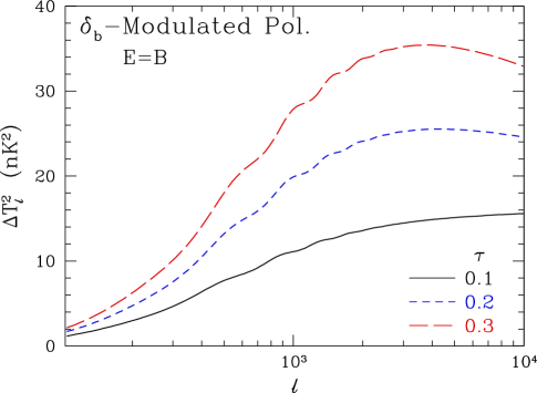
Likewise, the polarization follows from equation (63)

$$C_{\ell}^{EE}\!\!\! = \!\!\!C_{\ell}^{BB}={3\pi^{2}\over 50\ell^{3}}\int dD\,D_{A}\left({g\over X}\right)^{2}\Delta_{\delta_{b}}^{2}Q_{\rm rms}^{2}\,,$$ (75)

$$= \!\!\!{(2\pi)^{3/2}\over 200}\theta_{0}^{3}{D_{A}\delta D_{i}}{g^{2}\over X^{2}}e^{-{\ell^{2}\theta_{0}^{2}/2}}Q_{\rm rms}^{2}(D_{i})\,.$$

or

$${C_{\ell}^{EE}\over C_{\ell}^{\Theta\Theta}}={9\over 100}{Q_{\rm rms}^{2}\over v_{\rm rms}^{2}}\Big{|}_{D_{i}}\,.$$ (76)

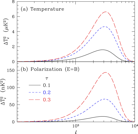
with $Q_{\rm rms}$ being either the primordial quadrupole of equation (48) or the kinematic quadrupole of equation (58). For adiabatic CDM models, the former typically dominates the latter even more so than for the density-modulated effect. The reason is that one no longer is weighted toward low redshifts and larger velocities by the growth of density perturbations. An example of the temperature and polarization signals for a specific choice of parameters is given in Fig. 12.

7. Discussion

We have explored the role of mildly-nonlinear density fluctuations in generating secondary CMB anisotropies and a host of contributions to the secondary polarization. In adiabatic CDM models, the Doppler effect from scattering off nonlinear baryonic clumps in a large-scale bulk flow is a natural extension of the Vishniac effect. In the small scale limit, the Vishniac effect simplifies to the corresponding effect for linear density perturbations. For this class of models, the nonlinear contributions out to overdensities of $\sim 10$ are comparable to or greater than the linear contributions, depending on the redshift of reionization. If the gas traces the dark matter to much higher overdensities then upto an order of magnitude increase in the subarcminute anisotropy would result. Likewise small-scale patchiness in the ionization can greatly increase the anisotropy in this regime. Calculations of the clumpiness of the ionized gas are difficult and unreliable even with state-of-the-art numerical simulations. An observational study of subarcminute scale anisotropies therefore offers the opportunity to discover aspects of reionization that are intractable to theoretical analysis today.

The secondary polarization from reionization is, as expected, extremely small in the context of adiabatic CDM models for structure formation and unlikely to inhibit extraction of even subtle effects such as the $B$-parity polarization from gravitational lensing or gravitational waves. It is worthwhile to note that these mechanisms generically predict comparable power in $E$ and $B$ parity polarization and may be important outside of the adiabatic CDM model context. For example, in a model with a coherent $1500$km s^-1 velocity field on the $100h^{-1}$Mpc scale the kinematically induced quadrupole generates a $B$-parity polarization at the $0.1\mu$K level for reasonable optical depths $\tau\sim 0.1-0.3$. Likewise, if the velocity field fell off less rapidly than $(1+z)^{-1/2}$ out to redshifts of order 10 or more, then the effect might also be enhanced to this level. In these models, the density and ionization modulation of the scattering produce even larger signals in the arcminute regime that may be observable. Thus even a null detection of $B$-parity polarization can be interesting. The tools that we have introduced in the text and appendix are quite general and have applications beyond the adiabatic CDM model.

Even in the adiabatic CDM class of models, significant uncertainties remain expecially in the contribution from inhomogeneities in the ionization and the small-scale behavior of the gas. These questions will ultimately be answered by the observations themselves as CMB experiments probe the arcminute regime with higher and higher sensitivity.

Appendix A Generalizing the Limber Equation

The Limber (1954) equation describes the two-point statistics of a field which is the two-dimensional projection on the sky of a three-dimensional source field whose statistical properties vary slowly along the line of sight. Kaiser (1992, 1998) expressed the result as a relation between the two and three dimensional power spectra of the fields. Hu & White (1996) generalized these flat-sky approximations in an all-sky approach for spatially flat cosmologies.

Here we extend the techniques in three ways. We generalize them to open cosmologies where Fourier analysis on the three-dimensional field is invalid. We allow for an arbitrary angular dependence in the source. Finally, we treat tensor fields on the sky in addition to the usual scalar fields.

A.1. Total Angular Momentum Method

A general field $X$ that depends both on position ${\bf x}$ and direction ${\bf n}$ at ${\bf x}$ can be expanded in a complete set of modes denoted ${}_{s}G_{j}^{m}$ (see Hu et al. 1998),

$$X({\bf x},{\bf n})=\int{d^{3}q\over(2\pi)^{3}}\sum_{\ell m}X_{\ell}^{(m)}{}_{s}G_{\ell}^{m}\,,$$ (A1)

where the spin index $s=0,\pm 2$ for scalar and tensor fields on the sky and ($\ell$,$m$) describe the multipole moments of the local angular dependence. In flat space, these modes are simply the product of plane waves and spin-spherical harmonics (Goldberg et al. 1967)

$${}_{s}G_{\ell}^{m} = (-i)^{\ell}\sqrt{4\pi\over 2\ell+1}{}_{s}Y_{\ell}^{m}(\hat{\bf n})\exp(i{\bf q}\cdot{\bf x})\,.$$ (A2)

Note that ${}_{0}Y_{\ell}^{m}=Y_{\ell}^{m}$, the ordinary spherical harmonics. The angular power spectrum of the field is defined as

$$C_{\ell}^{XX}=4\pi\int{d^{3}q\over(2\pi)^{3}}\sum_{m}{X_{\ell}^{(m)*}X_{\ell}^{(m)}\over(2\ell+1)^{2}}\,.$$ (A3)

Let us suppose that the field on the sky $X$ is generated by the line-of-sight integral of another positionally and directionally dependent field $S$ evaluated at a ${\bf x}=D\hat{\bf n}$

$$X({\bf x},{\bf n})\!\!\! = \!\!\!\int dD\,S({\bf x},{\bf n})\,,$$

$$= \!\!\!\int dD\,\int{d^{3}q\over(2\pi)^{3}}\sum_{jm}S_{j}^{(m)}{}_{s}G_{j}^{m}\,.$$

The normal modes can be rewritten in spherical coordinates as

$${}_{s}G_{j}^{m}=\sum_{\ell}(-i)^{\ell}\sqrt{4\pi(2\ell+1)}\alpha_{sj,\ell}^{(m)}\,{}_{s}Y_{\ell}^{m}\,,$$ (A5)

where we have used the spherical harmonic decomposition of a plane wave to combine the local and plane-wave angular dependence terms into the total angular dependence as seen by the observer at the origin. Here the $\alpha_{sj,\ell}^{(m)}$ are linear combinations of spherical Bessel functions with weights given by Clebsch-Gordan coefficients as we shall see. The moments of the field are then

$$X_{\ell}^{(m)}=\int dD\,(2\ell+1)\sum_{j}S_{j}^{(m)}\alpha_{sj,\ell}^{(m)}\,.$$ (A6)

For open geometries, the expressions in spherical coordinates take the same form except the radial functions $\alpha_{sj,\ell}^{(m)}$ are linear combinations of the hyperspherical Bessel functions $\Phi_{\ell}^{\nu}$ (Hu et al. 1998). They depend separately on radial distance

$$\chi=\Omega_{K}^{1/2}D\,,$$ (A7)

and wavenumber,

$$\nu={q\over H_{0}\Omega_{K}^{1/2}}\,,$$ (A8)

which itself differs from the usual eigenvalue $k$ of the Laplacian near the curvature scale

$$q=\sqrt{k^{2}-(|m|+1)H_{0}^{2}\Omega_{K}}\,.$$ (A9)

Useful radial functions include

$$\alpha_{00,\ell}^{(0)}\!\!\! = \!\!\!\Phi_{\ell}^{\nu}\,,$$

$$\alpha_{01,\ell}^{(1)}\!\!\! = \!\!\!\sqrt{\ell(\ell+1)\over 2(\nu^{2}+1)}{\rm csch}\chi\,\Phi_{\ell}^{\nu}\,,$$

$$\alpha_{02,\ell}^{(2)}\!\!\! = \!\!\!\sqrt{{3\over 8}{(\ell+2)(\ell^{2}-1)\ell\over(\nu^{2}+4)(\nu^{2}+1)}}{\rm csch}^{2}\chi\,\Phi_{\ell}^{\nu}\,,$$

$$\alpha_{01,\ell}^{(0)}\!\!\! = \!\!\!\sqrt{1\over\nu^{2}+1}\Phi_{\ell}^{\nu}{}^{\prime}\,,$$

$$\alpha_{02,\ell}^{(0)}\!\!\! = \!\!\!{1\over 2}\sqrt{1\over(\nu^{2}+4)(\nu^{2}+1)}\left[3\Phi_{\ell}^{\nu}{}^{\prime\prime}+(\nu^{2}+1)\Phi_{\ell}^{\nu}\right]\,,$$

$$\alpha_{02,\ell}^{(1)}\!\!\! = \!\!\!\sqrt{{3\over 2}{\ell(\ell+1)\over(\nu^{2}+4)(\nu^{2}+1)}}\left[{\rm csch}\chi\Phi_{\ell}^{\nu}(\chi)\right]^{\prime}\,.$$ (A10)

for $s=0$ and

$$\alpha_{\pm 22,\ell}^{(0)}\!\!\! = \!\!\!\sqrt{{3\over 8}{(\ell+2)(\ell^{2}-1)\ell\over(\nu^{2}+4)(\nu^{2}+1)}}{\rm csch}^{2}\chi\Phi_{\ell}^{\nu}\,,$$

$$\alpha_{\pm 22,\ell}^{(1)}\!\!\! = \!\!\!{1\over 2}\sqrt{(\ell-1)(\ell+2)\over(\nu^{2}+4)(\nu^{2}+1)}{\rm csch}\chi[({\rm coth}\chi\pm i\nu)\Phi_{\ell}^{\nu}$$

$$\!\!\!\quad+\Phi_{\ell}^{\nu}{}^{\prime}]\,,$$

$$\alpha_{\pm 22,\ell}^{(2)}\!\!\! = \!\!\!{1\over 4}\sqrt{1\over(\nu^{2}+4)(\nu^{2}+1)}[\Phi_{\ell}^{\nu}{}^{\prime\prime}+2(2{\rm coth}\chi\pm i\nu)\Phi_{\ell}^{\nu}{}^{\prime}$$ (A11)

$$\!\!\!\quad+(2{\rm coth}^{2}\chi+1-\nu^{2}\pm 4i\nu{\rm coth}\chi)\Phi_{\ell}^{\nu}]\,,$$

for $s=2$. Note that primes are derivatives with respect to $\chi$ and $\alpha_{sj,\ell}^{(-m)}=\alpha_{sj,\ell}^{(m)*}$.

A.2. Weak-Coupling Approximation

The weak-coupling approximation was introduced in Hu & White (1996) as a means of evaluating equation (A6) in the limit that the source $S_{j}^{(m)}$ varies in distance $D$ only on a much larger scale than the wavelength $q^{-1}$. In this case, the source may be taken out of the integral and evaluated at

$$D\!\!\! = \!\!\!\Omega_{K}^{-1/2}\sinh^{-1}(\Omega_{K}^{1/2}D_{A})\,,$$

$$D_{A}\!\!\! = \!\!\!(\ell+{1\over 2}){H_{0}\over q}\,.$$ (A12)

The remaining integral over $\alpha_{sj,\ell}^{(m)}$ becomes

$$\int_{0}^{\infty}dD\,\alpha_{sj,\ell}^{(m)}\!\!\! = \!\!\!{H_{0}\over q}{\sqrt{\pi}\over 2}{\Gamma[(\ell+1)/2]\over\Gamma[(\ell+2)/2]}W_{sj}^{(m)}K_{\nu}$$ (A13)

where the correction due to spatial curvature is given by

$$K_{\nu}=[1+{(\ell+1/2)^{2}\over\nu^{2}}]^{-1/4}\tanh^{1/2}({25\over 16}\nu).$$ (A14)

and the weights $W_{sj}^{(m)}$ follow from the radial functions (A10) and (A11):

$$W_{00}^{(0)}\!\!\! = \!\!\!1\,,$$

$$W_{01}^{(1)}\!\!\! = \!\!\!\sqrt{\ell(\ell+1)\over 2(\nu^{2}+1)}{\rm csch}\chi\,,$$

$$W_{02}^{(2)}\!\!\! = \!\!\!\sqrt{{3\over 8}{(\ell+2)(\ell^{2}-1)\ell\over(\nu^{2}+4)(\nu^{2}+1)}}{\rm csch}^{2}\chi\,,$$

$$W_{01}^{(0)}\!\!\! = \!\!\!0\,,$$

$$W_{02}^{(0)}\!\!\! = \!\!\!{1\over 2}\sqrt{(\nu^{2}+1)\over(\nu^{2}+4)}\,,$$

$$W_{02}^{(1)}\!\!\! = \!\!\!0\,,$$ (A15)

for the spin zero fields and

$$W_{\pm 22}^{(0)}\!\!\! = \!\!\!\sqrt{{3\over 8}{(\ell+2)(\ell^{2}-1)\ell\over(\nu^{2}+4)(\nu^{2}+1)}}{\rm csch}^{2}\chi\,,$$

$$W_{\pm 22}^{(1)}\!\!\! = \!\!\!{1\over 2}\sqrt{(\ell-1)(\ell+2)\over(\nu^{2}+4)(\nu^{2}+1)}{\rm csch}\chi$$ (A16)

$$\!\!\!\quad\times(\coth\chi\pm i\nu)\,,$$

$$W_{\pm 22}^{(2)}\!\!\! = \!\!\!{1\over 4}\sqrt{1\over(\nu^{2}+4)(\nu^{2}+1)}$$

$$\!\!\!\quad\times\left[(1-\nu^{2}+2\coth^{2}\chi)\pm 4i\nu\coth\chi\right]\,,$$

with

$${\rm csch}\chi=\nu/(\ell+1/2)\,.$$ (A17)

Where there are zero entries in these equations, a term of order $\dot{S}_{j}^{(m)}H_{0}/q$ exists and may be taken into account through integration by parts.

Note that the real part is the contribution to the “$E$”-parity of the tensor field and the imaginary part is the “$B$”-parity contribution. The flat limit is recovered as $\nu\rightarrow\infty$, $\chi\rightarrow 0$, and $\nu\chi\rightarrow kD/H_{0}$. We have numerically verified that the underlying expression for $\int dD\,\Phi_{\ell}^{\nu}$ is good to $\sim 1\%$ for $\ell\geq 2$ using the code of Kosowsky (1998).

A.3. Limber Formulation

The weak coupling approximation is a generalization of the familiar Limber equation as noted by Jaffe & Kamionkowski (1998). In the weak coupling approximation, we are left with a power spectrum defined as the integral over wavenumber $q$ in equation (A3). If we change variables to distance $D$ using the projection relation (A12) we obtain

$$C_{\ell}^{XX}\!\!\! = \!\!\!2\pi^{2}\int dDD_{A}F_{\ell}\sum_{m}|W_{sj}^{(m)}|^{2}\Delta_{S}^{2\,(jm)}\,,$$ (A18)

for a source with a single type of angular dependence $S_{j}^{(m)}$ and logarithmic power spectrum $\Delta_{S}^{2\,(jm)}$. The weighting in $\ell$ is

$$F_{\ell}\!\!\! = \!\!\!{1\over 2(\ell+1/2)^{2}}\left[{\Gamma[(\ell+1)/2]\over\Gamma[(\ell+2)/2]}\right]^{2}\tanh({25\over 16}{\ell+1/2\over\Omega_{K}^{1/2}D_{A}})$$ (A19)

$$\approx \!\!\!{1\over\ell^{3}}\,.$$

The approximation in the second line is for $\ell\gg 1$ where contributing modes are well below the curvature scale for reasonable cosmologies ($\nu\gg 1$). In this same limit, the weights also simplify,

$$\begin{array}[]{lll}W_{00}^{(0)}=1\,,&W_{01}^{(1)}=\sqrt{1\over 2}\,,&W_{02}^{(2)}=\sqrt{3\over 8}\,,\\ W_{01}^{(0)}=0\,,&W_{02}^{(0)}={1\over 2}\,,&W_{02}^{(1)}=0\,,\\ W_{\pm 22}^{(0)}=\sqrt{3\over 8}\,,&W_{\pm 22}^{(1)}=\pm{i\over 2}\,,&W_{\pm 22}^{(2)}=-{1\over 4}\,.\end{array}$$ (A20)

Notice that for the spin-2 case, $m=0,\pm 2$ produces a pure “$E$”-parity field and $m=\pm 1$ produces a pure “$B$” parity field, in contrast to the tight-coupling (delta function source approximation) where the power ratios between $B$ and $E$ are $0,6,8/13$ for $m=0,\pm 1,\pm 2$ (Hu & White 1997). For a simple source $S$ with no angular dependence ($j=0$, $m=0$) and a scalar field ($s=0$) on the sky, equation (A18) reduces to

$$C_{\ell}^{XX}=2{\pi^{2}\over\ell^{3}}\int dDD_{A}{\Delta^{2}_{S}}\,,$$ (A21)

which is the Fourier Limber equation as derived by Kaiser (1992; 1998).

Acknowledgements: I would like to thank D.J. Eisenstein, M. White, and M. Zaldarriaga for useful conversations. W.H. is supported by the Keck Foundation, a Sloan Fellowship, and NSF-9513835.

References

- (1) Abel, T., Norman, M.L., & Madau, P., preprint, astro-ph/9812151
- (2) Aghanim, N., Desert, F.X., Puget, J.L. & Gispert, R. 1996, A&A, 311, 1
- (3) Bouchet, F.R. & Gispert, R. 1999, astro-ph/9903176
- (4) Bunn, E.F. & White, M. 1997, ApJ, 480, 6
- (5) Carroll, S.M., Press, W.H., & Turner, E.L. 1992, ARA&A, 30, 499
- (6) Dodelson, S. & Jubas, J.M. 1995, ApJ, 439, 503
- (7) Eisenstein, D.J. & Hu, W. 1999, ApJ, 511, 5
- (8) Efstathiou, G. 1988, in Large Scale Motions in the Universe. A Vatican Study Week, ed. V.C. Rubin & G.V. Coyle (Princeton: Princeton University Press), 299
- (9) Gnedin, N. 1998, MNRAS, 299, 392
- (10) Gnedin, N. & Hui, L. 1998, MNRAS, 296, 44
- (11) Goldberg, J.N. 1967, J. Math. Phys., 7, 863
- (12) Griffiths, L.M., Barbosa, D., & Liddle, A.R., preprint, astro-ph/9812125
- (13) Gruzinov, A. & Hu, W. 1998, ApJ, 508, 435
- (14) Gunn, J.E. & Peterson, B.A. 1965, ApJ, 142, 1633
- (15) Haiman, Z. & Knox, L., preprint, astro-ph/9902311
- (16) Hamilton, A.J.S., Kumar, P., Lu, E. & Matthews, A. 1991 ApJ, 374, L1
- (17) Hu, W. & Sugiyama, N. 1995, ApJ, 444, 489
- (18) Hu, W. & White, M. 1996, A&A, 315, 33
- (19) Hu, W. & White, M. 1997, Phys. Rev. D, 56, 596
- (20) Hu, W., Seljak, U., White, M. & Zaldarriaga, M. 1998, Phys. Rev. D, 57, 3290
- (21) Kaiser, N. 1984, ApJ, 282, 374
- (22) Kaiser, N. 1992, ApJ, 388, 272
- (23) Kaiser, N. 1998, ApJ, 498, 26
- (24) Kamionkowski, M., Kosowsky, A., & Stebbins, A. 1997, Phys. Rev. D, 55, 7368
- (25) Knox, L., Scoccimarro, R., & Dodelson, S. 1998, Phys. Rev. Lett., 81, 2004
- (26) Kofman, L.A. & Starobinskii, A.A. 1985, Sov. Astron. Lett., 9, 643
- (27) Kosowsky, A., astro-ph/9805173
- (28) Jaffe, A.H. & Kamionkowski, M. 1998, Phys.Rev. D, 58, 043001
- (29) Lauer, T. & Postman, M. 1994, ApJ, 425, 418
- (30) Limber, D. 1954, ApJ, 119, 655
- (31) Miralda-Escude, J., Haehnelt, M. & Rees, M.J. 1999, ApJ (submitted, astro-ph/9812306)
- (32) Ostriker, J.P., & Vishniac, E.T. 1986, ApJ, 306, 51
- (33) Peacock, J.A. & Dodds, S.J. 1994, MNRAS, 267, 1020
- (34) Peacock, J.A. & Dodds, S.J. 1996, MNRAS, 280, L19
- (35) Peebles, P.J.E. 1980, The Large-Scale Structure of the Universe, (Princeton: Princeton Univ. Press)
- (36) Persi, F.M., Spergel, D.N., Cen, R., & Ostriker, J.P. 1995, ApJ, 442, 1
- (37) Scoccimarro, R., Zaldarriaga, M. & Hui, L. 1999, ApJ (in press, astro-ph/9901099)
- (38) Seljak, U. & Zaldarriaga, M. 1996, ApJ, 469, 437
- (39) Sunyaev, R.A. & Zel’dovich, Ya. B. 1980, MNRAS, 190, 413
- (40) Tegmark, M., Eisenstein, D.J., Hu, W., de Oliviera-Costa, A., preprint, astro-ph/9905257
- (41) Vishniac, E.T. 1987, ApJ, 322, 597
- (42) White, M. & Scott, D. 1996, ApJ, 459, 415
- (43) Zaldarriaga, M. & Seljak, U. 1997, Phys. Rev. D. 55, 1830
- (44) Zaldarriaga, M. & Seljak, U. 1998, Phys. Rev. D. 58, 023003