Computational Methods for Nucleosynthesis and Nuclear Energy Generation

Abstract

This review concentrates on the two principle methods used to evolve nuclear abundances within astrophysical simulations, evolution via rate equations and via equilibria. Because in general the rate equations in nucleosynthetic applications form an extraordinarily stiff system, implicit methods have proven mandatory, leading to the need to solve moderately sized matrix equations. Efforts to improve the performance of such rate equation methods are focused on efficient solution of these matrix equations, by making best use of the sparseness of these matrices. Recent work to produce hybrid schemes which use local equilibria to reduce the computational cost of the rate equations is also discussed. Such schemes offer significant improvements in the speed of reaction networks and are accurate under circumstances where calculations with complete equilibrium fail.

1 Introduction

By the second half of the last century, work by Helmholtz, Kelvin and others made it clear that neither gravity nor any other then known energy source could account for the age of the sun and solar system, as determined by geological measurements. Following quickly on the heels of Rutherford’s 1911 discovery of the atomic nucleus, Eddington and others suggested that nuclear transmutations might be the remedy to this quandary. With the burgeoning knowledge of the properties of nuclei and nuclear reactions in the 1930s, 1940s and 1950s, came a growing understanding of the role that individual nuclear reaction played in the synthesis of the elements. In 1957, Burbidge, Burbidge, Fowler & Hoyle [1] and Cameron [2] wove these threads into a cohesive theory of nucleosynthesis, demonstrating how the solar isotopic abundances (displayed in Fig. 1) bore the fingerprints of their astrophysical origins. Today, investigations refine our answers to these same two questions, how are the elements that make up our universe formed, and how do these nuclear transformations, and the energy they release, affect their astrophysical hosts.

In this article, we will concentrate on summarizing the two basic numerical methods used in nucleosynthesis studies, the tracking of nuclear transmutations via rate equations and via equilibria. We will also briefly discuss work which seeks to meld these methods together in order to overcome the limitations of each. To properly orient readers unfamiliar with nuclear astrophysics and to briefly describe the differing physical conditions which influence the optimal choice of abundance evolution method, we begin with a brief introduction to the background astrophysics (§2), before discussing the form that the rate equations take (§3). In §4 we will discuss the difficulties inherent in solving these rate equations. §5 describes the equations of nuclear equilibria as well as the limitations of their use. Finally in §6 we will discuss hybrid schemes which seek to use local equilibria to simplify the rate equations.

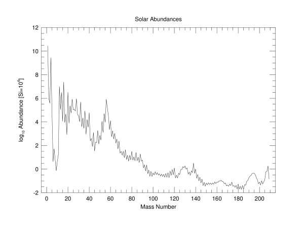
Figure 1: The abundances of isotopes in the solar system as a function of atomic mass [3, 4]. The abundances are normalized so that the total abundance of silicon is $10^{6}$.

2 Nuclear Processes in Astrophysics

In general, nucleosynthesis calculations divide into two categories, (1) nucleosynthesis during the hydrostatic burning stages of stellar evolution and (2) nucleosynthesis in explosive events. The critical distinction between the categories is the timescale over which transmutations occur. In hydrostatic burning, the release of nuclear energy occurs at a rate balancing the loss of energy via radiation and neutrinos (the photon and neutrino luminosities), providing continuous pressure support against the star’s self-gravity. This results in slow burning at relatively low temperatures and densities. In explosive nucleosynthesis the timescale and thermodynamic conditions are determined by the hydrodynamics. For example, in many cases of interest, a detonation shock heats the material and expels it outward, to cool adiabatically as it expands. In such a case, the limiting timescale is that of the hydrodynamic expansion, not those intrinsic to the nuclear processes. Though constrained from an in depth discussion by our concentration on the computational methods, in this section we will outline the physics of the many burning stages and in particular the way that the physics influences the choice of method for computing the abundance changes.

2.1 Hydrostatic Burning Stages in Stellar Evolution

A star shines bright because, deep in its core, energy released by thermonuclear reactions balances the star’s self-gravity. Table 1 lists the series of burning stages which make up a star’s life, with their representative conditions for a star like the sun and a star 20 times more massive (M=20 $M_{\odot}$). With the consumption in turn of each nuclear fuel, the inexorable squeeze of gravity creates higher temperatures and densities. The initiation of each subsequent stage requires these progressively higher temperatures and densities to overcome the increasing Coulomb repulsion of the reactants. Around the core, layers of progressively lighter matter echo prior central burning stages. A star’s mass is the most important determinant of its final destiny, with less massive stars not progressing through the full sequence of burning stages. For stars with masses less than 8 $M_{\odot}$, helium burning is the final burning stage, because the packing of electrons into a degenerate Fermi-Dirac configuration provides sufficient pressure support to prevent further contraction. Instead, the remaining envelope is driven off, forming a planetary nebula, and leaving the bare core. Such cooling bare cores, composed of C & O in this case, or He or O, Ne & Mg in others, are termed white dwarf stars. As examination of Table 1 reveals, in less massive stars the individual burning stages which occur do so at higher density, lower temperature and over much longer timescales. For a more exhaustive description of stellar evolution consult, e.g., [5, 6, 7]

Table 1: Stellar Burning Stages

Burning	$\rho_{c}$	$T_{c}$	$\tau$	$L_{phot}$	$L_{\nu}$	Primary
Stage	($\mathrm{\thinspace g\thinspace cm^{-3}}$)	($\mathrm{\thinspace GK}$)	(yr)	($\mathrm{\thinspace ergs/s}$)	($\mathrm{\thinspace ergs/s}$)	Reactions
For a 1 $M_{\odot}$star [8]
Hydrogen	150	0.015	1$\times 10^{10}$	3.9$\times 10^{33}$	-	PP chain
Helium	2.0$\times 10^{5}$	0.15	4 $\times 10^{8}$	1.6$\times 10^{35}$	-	Triple $\alpha$
For a 20 $M_{\odot}$star [9]
Hydrogen	5.6	0.040	1.0$\times 10^{7}$	2.7$\times 10^{38}$	-	CNO Cycle
Helium	9.4$\times 10^{2}$	0.19	9.5$\times 10^{5}$	5.3$\times 10^{38}$	$<\times 10^{36}$	Triple $\alpha$
Carbon	2.7$\times 10^{5}$	0.81	3.0$\times 10^{2}$	4.3$\times 10^{38}$	7.4$\times 10^{39}$	$\mathrm{{}^{12}C}+\mathrm{{}^{12}C}\rightarrow\mathrm{{}^{20}Ne}+\alpha$
Neon	4.0$\times 10^{6}$	1.7	0.4	4.4$\times 10^{38}$	1.2$\times 10^{43}$	$\mathrm{{}^{20}Ne}+\gamma\rightarrow\mathrm{{}^{16}O}+\alpha$
Oxygen	6.0$\times 10^{6}$	2.1	0.5	4.4$\times 10^{38}$	7.4$\times 10^{43}$	$\mathrm{{}^{16}O}+\mathrm{{}^{16}O}\rightarrow\mathrm{{}^{28}Si}+\alpha$
Silicon	4.9$\times 10^{7}$	3.7	0.01	4.4$\times 10^{38}$	3.1$\times 10^{45}$	$\mathrm{{}^{28}Si}+7\alpha\rightarrow\mathrm{{}^{56}Ni}$

Because the hydrostatic burning timescales are long compared to beta-decay half-lives (with a few exceptions of long-lived unstable nuclei), nuclei can decay back to stability before undergoing the next reaction. As a result, most reactions in hydrostatic burning stages proceed through stable nuclei. As indicated in Table 1, stars transmute hydrogen into helium via two alternative reaction sequences; the PP-chains, initiated by the conversion of two protons to a positron, a neutrino and a deuteron, (commonly notated $\mathrm{{}^{1}H}(p,e^{+}\nu)\mathrm{{}^{2}H}$), and the CNO cycle, which converts ¹H into ⁴He by a sequence of catalytic ($p,\gamma$) and ($p,\alpha$) reactions on pre-existing C, N, and O nuclei and subsequent beta-decays. He-burning follows H-burning, converting $\mathrm{{}^{4}He}$ into $\mathrm{{}^{12}C}$ via the triple-alpha process, which we will discuss further in §6. A portion (larger in more massive stars) of these $\mathrm{{}^{12}C}$ nuclei capture an additional $\alpha$-particle to form $\mathrm{{}^{16}O}$. With the exhaustion of $\mathrm{{}^{4}He}$, contraction continues until conditions are sufficient to fuse pairs of $\mathrm{{}^{12}C}$ nuclei, producing $\mathrm{{}^{20}Ne}$ and a small fraction of $\mathrm{{}^{23}Na}$. Depletion of $\mathrm{{}^{12}C}$ is followed by further contraction. Before temperatures become sufficient for $\mathrm{{}^{16}O}$ nuclei to fuse, the thermal photon bath becomes energetic enough to photodisintegrate $\mathrm{{}^{20}Ne}$ (see §3.1 and Eq. 8 for more details), freeing an $\alpha$-particle which can be captured by other $\mathrm{{}^{20}Ne}$ nuclei forming $\mathrm{{}^{24}Mg}$. Once $\mathrm{{}^{20}Ne}$ is exhausted, continued contraction raises the temperature until it is sufficient for $\mathrm{{}^{16}O}$ to fuse, producing $\mathrm{{}^{28}Si}$ and $\mathrm{{}^{31}P}$.

Si-burning, like Ne-burning, is initiated by photodisintegration reactions which then provide the light particles needed for capture reactions. Temperatures sufficient to photodisintegrate Si are also sufficient to photodisintegrate all other nuclei and permit charged particle captures (and, in any case, neutron captures, where there is no Coulomb barrier to overcome). This leaves many individual reactions in a chemical equilibrium where reactions are balanced by their inverses. If each of the important reactions connecting two species is in chemical equilibrium, then the relative abundances of these species will obey an equilibrium distribution. As the most bound nuclei, and therefore most resistant to photodisintegration, isotopes of Fe and Ni dominate the products of silicon burning, producing the Fe-peak seen near $A=60$ in Fig 1. We will discuss this equilibrium further in §5. For a more complete description of silicon burning, see [10, 11]. It is important to note that because of the large photodisintegration fluxes which nearly balance their reverse capture reactions, the effective rate at which silicon is burned is as much as $10^{5}$ times slower than the individual reaction rates would indicate. This near balance of reaction rates during silicon burning will also prove important in our discussion of numerical methods in §6. More extensive overviews of the major and minor reaction sequences in all burning stages from helium to silicon burning in massive stars is given in [7, 12, 13, 14, 15].

An additional hydrostatic nucleosynthetic process is the s(low neutron capture)-process. While energetically unimportant, this slow neutron capture process leads to the build-up of the (small) abundances of roughly half of the heavy elements. During core and shell He-burning, $(\alpha,n)$ reactions on neutron rich nuclei provide a source of free neutrons, initiating a series of neutron captures and $\beta$-decays, starting on pre-existing medium and heavy nuclei (up to Fe), synthesizing nuclei up to Pb and Bi. Such reactions, occurring under temperature conditions where photodisintegration are unimportant, approach a steady flow, wherein the flux of $\mathrm{{}^{A-1}Z}(n,\gamma)\mathrm{{}^{A}Z}$ equals the flux of $\mathrm{{}^{A}Z}(n,\gamma)\mathrm{{}^{A+1}Z}$, as long as the relevant reaction timescale is short in comparison to the process timescale. For general overviews of the s-process see [16, 17, 18, 19]. From a numerical perspective, in this and several other cases, it is often advantageous to couple only the dominant energy producing reactions to the hydrodynamics and perform detailed nucleosynthesis, which can require a very large nuclear network, in a post-processing fashion.

2.2 Explosive Burning

While hydrostatic sources are capable of producing many of the isotopes shown in Fig. 1, most of these products are trapped deep in the potential well of their parent star or white dwarf. Explosions are necessary to liberate the transmuted nuclei from this gravitational embrace. In massive stars, the formation of the iron core during silicon burning marks the end of nuclear energy generation in the core, as nuclei more massive than the iron peak nuclei are less bound. Ultimately, gravitational contraction turns into collapse, which is halted suddenly by degenerate nucleon pressure when the matter density approaches or exceeds that of the atomic nucleus $(\sim 10^{14}\mathrm{\thinspace g\thinspace cm^{-3}})$. Infalling material from overlying layers bounce off of this newly formed proto-neutron star, sending a shockwave outward. Though this shock soon stalls, it is re-invigorated by neutrinos carrying off the gravitational energy released in the formation of the proto-neutron star (see, e.g., [20, this volume]). This re-energized shock propagates out of the star, unbinding much of the overlying layers and driving them into space with velocities of thousands of $\mathrm{\thinspace km/s}$, and producing a (core-collapse) supernova [9, 21, 22]. This passing shock also causes further nucleosynthesis to occur as it passes through the layered composition of the star, raising temperatures to several $\mathrm{\thinspace GK}$. Many of the hydrostatic burning processes discussed in §2.1 occur under these explosive conditions but at much higher temperatures and over much shorter timescales. With little regard to the initial composition, the burning stage which determines the nucleosynthetic outcome is that whose timescale at the peak temperature is comparable to the hydrodynamic timescale (see, e.g., [23, 24, 25]). Much more detail on the products of explosive burning in core collapse supernova is available in the literature (see, e.g., [7, 14, 15, 25, 26, 27]). Because these explosive burning stages are responsible for producing many nuclei with masses between 16-70, detailed modeling is important. However such modeling is complicated by the strongly varying hydrodynamic conditions. The computational feasibility of performing detailed nucleosynthesis calculations (particularly explosive silicon burning) within the latest generation of multi-dimensional hydrodynamic models is greatly aided by techniques like those we will discuss in §6.1

The explosive analogue of the s-process is the r(apid neutron capture)-process which requires larger neutron concentrations. Conditions suitable for r-process nucleosynthesis can occur in the decompression of neutron star matter [28, 29, 30, 31, 32] or in the innermost regions of the core-collapse supernova ejecta [33, 34]. As a result of the electron and neutrino captures this material has experienced, there are more neutrons than protons. With equal numbers of protons and neutrons tied up in $\mathrm{{}^{4}He}$, the remainder provide the required neutron to heavy seed nucleus ratio. Calculations independent of the specific astrophysical site [35, 36], performed with the goal of reproducing the solar abundance pattern of heavy elements, show that extremely unstable nuclei close to the neutron drip line are produced and beta-decay timescales can be short in comparison to the process timescales. Because of the large number of nuclei involved, r-process calculations are among the most numerically expensive, however as we will discuss in §4 & §6, partial equilibria and/or the slow variation of the light particle abundances can be employed to simplify the calculation.

A second type of supernova is the thermonuclear supernova, which occurs when explosive carbon burning is ignited in the center of an accreting white dwarf, either as a result of the white dwarf exceeding the maximum mass ($\sim 1.4M_{\odot}$) which can be supported by electron degeneracy pressure (see, e.g., [37, 38, 39, 40, 41]) or due to compression resulting from the detonation of an accreted He layer (see, e.g., [42, 43]). In either case, a flame front propagates outward disrupting the white dwarf and leaving a composition dominated by iron peak and intermediate mass nuclei. Computationally, in addition to sharing the complications discussed for explosive burning in core collapse supernovae, explosive nucleosynthesis in these thermonuclear supernovae is also the source of the energy which powers the explosion. Thus accurate hydrodynamic simulation requires at least the inclusion of an accurate means to calculate the rate of thermonuclear energy release.

If a white dwarf accretes hydrogen (typically via mass transfer from a binary companion) slowly enough, a layer of unburned hydrogen will build up on the surface of the white dwarf. Once the density of this layer is sufficient to ignite the hydrogen, a nova results (see, e.g., [44, 45, 46]). The degeneracy of the material and the steep gravitational gradients at the surface of the white dwarf, result in explosive hydrogen burning via the “hot” or $\beta$-limited CNO cycle [47, 48], releasing $10^{46}-10^{47}\mathrm{\thinspace ergs}$ over timescales of 100-1000 s, with peak temperatures reaching $0.2-0.3\mathrm{\thinspace GK}$. A neutron star can also accrete mass from a companion in a similar fashion, building up a layer of hydrogen which explodes to produce an X-ray burst (see, e.g., [49, 50]). Because the neutron stars surface gravitational gradients are even stronger, the timescales are shorter (1-10 s) and even higher peak temperatures ($1-2\mathrm{\thinspace GK}$) are reached, enabling proton capture up to and beyond the Fe-peak, the r(apid) p(roton capture)-process [47, 51]. However the size of the hydrogen layer is much smaller (as small as $10^{-12}M_{\odot}$) and, as a result, so is the energy release, which is typically $10^{39}-10^{40}\mathrm{\thinspace ergs}$. The thermonuclear source of the explosive energy in novae and X-ray burst, as well as the similarity in the convective and nuclear timescales, require that hydrodynamic simulations of these objects include large networks. Fortunately, approximations (which we will discuss in §6) exist which can greatly reduce the computational cost.

An additional form of explosive burning occurred as the universe expanded from its primordial Big Bang. Since its origin, the universe has been expanding, cooling from the initially extreme temperatures. At the earliest times, the populations of all kinds of sub-atomic particles were equilibrated. Eventually, continued cooling and the freezeout of this equilibrium left only a few neutrons and protons (approximately one baryon per billion photons) with approximately 7 protons per neutron. These nucleons largely remained free because the small Q-value of the reaction $n+p\rightleftharpoons\mathrm{{}^{2}H}+\gamma$ permits chemical equilibrium to persist to temperatures of 1 $\mathrm{\thinspace GK}$, keeping the abundance of deuterium very small. By the time the universe has cooled to 1 $\mathrm{\thinspace GK}$, the expansion has reduced the density to $\sim 10^{-5}\mathrm{\thinspace g\thinspace cm^{-3}}$, a density small enough that, even with an expansion timescale of days, the resulting tiny flux through the $3\alpha$ reaction did not produce significant amounts of heavy elements. Instead Big Bang nucleosynthesis is responsible for the production of the lightest elements; $\mathrm{{}^{1}H}$, $\mathrm{{}^{4}He}$, $\mathrm{{}^{2}H}$, $\mathrm{{}^{3}He}$ and $\mathrm{{}^{7}Li}$ [52, 53]. In principle, the small number of affected species and the simple hydrodynamic evolution make Big Bang nucleosynthesis the least computationally challenging. However the greater accuracy of the relevant nuclear reactions, as well as the important limits that Big Bang nucleosynthesis calculations place on cosmologically important factors, have resulted in a much stronger drive to high precision in Big Bang nucleosynthesis calculations [54, 55].

3 Thermonuclear Reaction Networks

From the discussion in the preceding section, it is clear that nuclear abundances in many cases obey equilibrium distributions. But the general case requires the evolution of nuclear abundances via a nuclear reaction network. Composed of a system of first order differential equations, the nuclear reaction network has sink and source terms representing each of the many nuclear reactions involved. Prior to discussing the numerical difficulties posed by the nuclear network, it is necessary to understand the sets of equations we are attempting to solve. To this end, we present a brief overview of the thermonuclear reaction rates of interest and how these rates are assembled into the differential equations we must ultimately solve. For more detailed information, we refer the reader to a number of more complete discussions [5, 7, 56, 57, 58] which can be found in the literature. We will end this section by briefly discussing the coupling of nucleosynthesis with hydrodynamics.

3.1 Thermonuclear Reaction Rates

There are a large number of types of nuclear reactions which are of astrophysical interest. In addition to the emission or absorption of nuclei and nucleons, nuclear reactions can involve the emission or absorption of photons ($\gamma$ -rays) and leptons (electrons, neutrinos, and their anti-particles). As a result, nuclear reactions involve three of the four fundamental forces, the nuclear strong, electromagnetic and nuclear weak forces. Reactions involving leptons (termed weak interactions) proceed much more slowly than those involving only nucleons and photons. However these reactions are still important, as only weak interactions can change the global ratio of protons to neutrons.

The most basic piece of information about any nuclear reaction is the nuclear cross section. The cross section for a reaction between target $j$ and projectile $k$ is defined by

$$\sigma={\rm{number\ of\ reactions\ target^{-1}sec^{-1}}\over{flux\ of\ incoming\ projectiles}}={{r/n_{j}}\over{n_{k}v}}.$$ (1)

The second equality holds when the relative velocity between targets of number density $n_{j}$ and projectiles of number density $n_{k}$ is constant and has the value $v$. Then $r$, the number of reactions per $\mathrm{cm^{3}}$ and sec, can be expressed as $r=\sigma vn_{j}n_{k}$. More generally, the targets and projectiles have distributions of velocities, in which case $r$ is given by

$$r_{j,k}=\int\sigma(|\vec{v}_{j}-\vec{v}_{k}|)|\vec{v}_{j}-\vec{v}_{k}|d^{3}n_{j}d^{3}n_{k}.$$ (2)

The evaluation of this integral depends on the types of particles and distributions which are involved. For nuclei $j$ and $k$ in an astrophysical plasma, Maxwell-Boltzmann statistics generally apply, thus

$$d^{3}n=n({{m}\over{2\pi k_{B}T}})^{3/2}\exp(-{{mv^{2}}\over{2k_{B}T}})d^{3}v,$$ (3)

allowing $n_{j}$ and $n_{k}$ to be moved outside of the integral. Eq. 2 can then be written as $r_{j,k}={\langle\sigma v\rangle}_{j,k}n_{j}n_{k}$, where $\langle\sigma v\rangle$ is the velocity integrated cross section. Equivalently, one can express the reaction rate in terms of a mean lifetime of particle $j$ against destruction by particle $k$,

$$\tau_{k}(j)={1\over{{\langle\sigma v\rangle}_{j,k}n_{k}}}$$ (4)

For thermonuclear reactions, these integrated cross sections have the form [5, 59]

$$\langle j,k\rangle\equiv{\langle\sigma v\rangle}_{j,k}=({8\over{\mu\pi}})^{1/2}(k_{B}T)^{-3/2}\int_{0}^{\infty}E\sigma(E){\rm exp}(-E/k_{B}T)dE,$$ (5)

where $\mu$ denotes the reduced mass of the target-projectile system, $E$ the center of mass energy, $T$ the temperature and $k_{B}$ is Boltzmann’s constant.

Experimental measurements and theoretical predictions for these reaction rates provide the data input necessary for nuclear networks. While detailed discussion of individual rates is beyond the scope of this article, the interested reader is directed to the following reviews. Experimental nuclear rates have been reviewed in detail by [56, 60, 61]. The most recent experimental charged particle rate compilations are the ones by [62, 63]. Experimental neutron capture cross sections are summarized by [64, 65, 18]. Rates for unstable (light) nuclei are given, for example, by [51, 53, 66, 67, 68, 69]. For the vast number of medium and heavy nuclei which exhibit a high density of excited states at capture energies, Hauser-Feshbach (statistical model) calculations are applicable. The most recent compilations were provided by [70, 71, 72, 73]. Improvements in level densities [74], alpha potentials, and the consistent treatment of isospin mixing will lead to the next generation of theoretical rate predictions [75, 76].

In practice, these experimental and theoretical reaction rates are determined for bare nuclei, while in astrophysical plasmas, these reactions occur among a background of other nuclei and electrons. As a result of this background, the reacting nuclei experience a Coulomb repulsion modified from that of bare nuclei. For high densities and/or low temperatures, the effects of this screening of reactions becomes very important. Under most conditions (with non-vanishing temperatures) the generalized reaction rate integral can be separated into the traditional expression without screening [Eq. 5] and a screening factor,

$$\langle j,k\rangle^{*}=f_{scr}(Z_{j},Z_{k},\rho,T,n_{i})\langle j,k\rangle.$$ (6)

This screening factor is dependent on the charge of the involved particles, the density, temperature, and the composition of the plasma. For more details on the form of $f_{scr}$, see, e.g., [77, 78, 79, 80, 81]. At high densities and low temperatures screening factors can enhance reactions by many orders of magnitude and lead to pycnonuclear ignition. In the extreme case of very low temperatures, where reactions are only possible via ground state oscillations of the nuclei in a Coulomb lattice, Eq. 6 breaks down, because it was derived under the assumption of a Boltzmann distribution (for recent references, see [81, 82]).

When particle $k$ in Eq. 2 is a photon, the distribution $d^{3}n_{k}$ is given by the Plank distribution,

$$d^{3}n_{\gamma}={{8\pi}\over{c^{3}h^{3}}}{{E_{\gamma}^{2}}\over{\exp\left(E_{\gamma}/k_{B}T\right)-1}}dE_{\gamma}\ .$$ (7)

Furthermore, the relative velocity is always $c$ and thus the integral is separable, simplifying to

$$r_{j}={{\int d^{3}n_{j}}\over{\pi^{2}(c\hbar)^{3}}}\int_{0}^{\infty}{{c\sigma(E_{\gamma})E_{\gamma}^{2}}\over{{\rm exp}(E_{\gamma}/k_{B}T)-1}}dE_{\gamma}\equiv\lambda_{j,\gamma}(T)n_{j}.$$ (8)

In practice there is, however, no need to directly evaluate the photodisintegration cross sections, because they can be expressed by detailed balance in terms of the capture cross sections for the inverse reaction, $l+m\rightarrow j+\gamma$ [59].

$$\lambda_{j,\gamma}(T)=({{G_{l}G_{m}}\over G_{j}})({{A_{l}A_{m}}\over A_{j}})^{3/2}({{m_{u}k_{B}T}\over{2\pi\hbar^{2}}})^{3/2}\langle l,m\rangle\exp(-Q_{lm}/k_{B}T).$$ (9)

This expression depends on the partition functions, $G_{k}=\sum_{i}(2J_{i}+1)\exp(-E_{i}/k_{B}T)$ (which account for the populations of the excited states of the nucleus), the mass numbers, $A$, the temperature $T$, the inverse reaction rate $\langle l,m\rangle$, and the reaction $Q$-value (the energy released by the reaction), $Q_{lm}=(m_{l}+m_{m}-m_{j})c^{2}$. Since photodisintegrations are endoergic, their rates are vanishingly small until sufficient photons exist in the high energy tail of the Planck distribution with energies $>Q_{{lm}}$. As a rule of thumb this requires $T$$\approx$$Q_{lm}/30k_{B}$.

A procedure similar to that for Eq. 8 applies to captures of electrons by nuclei. Because the electron is 1836 times less massive than a nucleon, the velocity of the nucleus $j$ in the center of mass system is negligible in comparison to the electron velocity ($|\vec{v}_{j}-\vec{v}_{e}|\approx|\vec{v}_{e}|$). In the neutral, completely ionized plasmas typical of the astrophysical sites of nucleosynthesis, the electron number density, $n_{e}$, is equal to the total density of protons in nuclei, $\sum_{i}Z_{i}n_{i}$. However in many of these astrophysical settings the electrons are at least partially degenerate, therefore the electron distribution cannot be assumed to be Maxwellian. Instead the capture cross section has to be integrated over a Boltzmann, partially degenerate, or degenerate Fermi distribution of electrons, depending on the astrophysical conditions. The resulting electron capture rates are functions of $T$ and $n_{e}$,

$$r_{j}=\lambda_{j,e}(T,n_{e})n_{j}.$$ (10)

Similar equations apply for the capture of positrons which are in thermal equilibrium with photons, electrons, and nuclei. Electron and positron capture calculations have been performed by [83, 84, 85] for a large variety of nuclei with mass numbers between A=20 and A=60. For improvements and application to heavier nuclei see also [86, 87, 88, 89].

For normal decays, like beta or alpha decays, with a characteristic half-life $\tau_{1/2}$, Eq. 8 & 10 also applies, with the decay constant $\lambda_{j}=\ln 2/\tau_{1/2}$. In addition to innumerable experimental half-life determinations, beta-decay half-lives for unstable nuclei have been predicted by [90, 91] & [92, including temperature effects]. More recently, estimates have been made with improved quasi particle RPA calculations [93, 94, 95, 96, 97, 98, 99, 100].

At high densities ($\rho\sim 10^{13}\mathrm{\thinspace g\thinspace cm^{-3}}$), even though the size of the neutrino scattering cross section on nuclei and electrons is very small, enough scattering events occur to thermalize the neutrino distribution. Under such conditions the inverse process to electron capture (neutrino capture) can occur in significant numbers and the neutrino capture rate can be expressed in a form similar to Eqs. 8 & 10 by integrating over the thermal neutrino distribution (e.g. [101]). Inelastic neutrino scattering on nuclei can also be expressed in this form. The latter can cause particle emission, similar to photodisintegration (e.g. [102, 103, 104, 105, 106]). The calculation of these rates can be further complicated by the neutrinos not being in thermal equilibrium with the local environment. When thermal equilibrium among neutrinos was established at a different location, then the neutrino distribution might be characterized by a chemical potential and a temperature different from the local values. Otherwise, the neutrino distribution must be evolved in detail [20, this volume].

3.2 Thermonuclear Rate Equations

The large number of reaction types discussed in §3.1 can be divided into 3 functional categories based on the number of reactants which are nuclei. The reactions involving a single nucleus, which include decays, electron and positron captures, photodisintegrations, and neutrino induced reactions, depend on the number density of only the target species. For reaction involving two nuclei, the reaction rate depends on the number densities of both target and projectile nuclei. There are also a few important three-particle process, like the triple-$\alpha$ process discussed in §6, which are commonly successive captures with an intermediate unstable target (see, e.g., [107, 108]). Using an equilibrium abundance for the unstable intermediate, the contributions of these reactions are commonly written in the form of a three-particle processes, depending on a trio of number densities. Grouping reactions by these 3 functional categories, the time derivatives of the number densities of each nuclear species in an astrophysical plasma can be written in terms of the reaction rates, $r$, as

$$\left.{{\partial n_{i}}\over{\partial t}}\right|_{\rho=const}=\sum_{j}\mathcal{N}^{i}_{j}r_{j}+\sum_{j,k}\mathcal{N}^{i}_{j,k}r_{j,k}+\sum_{j,k,l}\mathcal{N}^{i}_{j,k,l}r_{j,k,l},$$ (11)

where the three sums are over reactions which produce or destroy a nucleus of species $i$ with 1, 2 & 3 reactant nuclei, respectively. The $\mathcal{N}$ s provide for proper accounting of numbers of nuclei and are given by: $\mathcal{N}^{i}_{j}=N_{i}$, $\mathcal{N}^{i}_{j,k}=N_{i}/\prod_{m=1}^{n_{m}}|N_{j_{m}}|!$, and $\mathcal{N}^{i}_{j,k,l}=N_{i}/\prod_{m=1}^{n_{m}}|N_{j_{m}}|!$. The $N_{i}^{\prime}s$ can be positive or negative numbers that specify how many particles of species $i$ are created or destroyed in a reaction, while the denominators, including factorials, run over the $n_{m}$ different species destroyed in the reaction and avoid double counting of the number of reactions when identical particles react with each other (for example in the $\mathrm{{}^{12}C}$ + $\mathrm{{}^{12}C}$ or the triple-$\alpha$ reactions; for details see [59]).

In addition to nuclear reactions, expansion or contraction of the plasma can also produce changes in the number densities $n_{i}$. To separate the nuclear changes in composition from these hydrodynamic effects, we introduce the nuclear abundance $Y_{i}=n_{i}/\rho N_{A}$, where $N_{A}$ is Avagadro’s number. For a nucleus with atomic weight $A_{i}$, $A_{i}Y_{i}$ represents the mass fraction of this nucleus, therefore $\sum A_{i}Y_{i}=1$. Likewise, the equation of charge conservation becomes $\sum Z_{i}Y_{i}=Y_{e}$, where $Y_{e}(=n_{e}/\rho N_{A})$ is the electron abundance. By recasting Eq. 11 in terms of nuclear abundances $Y_{i}$, a set of ordinary differential equations for the evolution of $\dot{Y}_{i}$ results which depends only on nuclear reactions. In terms of the reaction cross sections introduced in §3.1, this reaction network is described by the following set of differential equations

$$\dot{Y}_{i} = \sum_{j}\mathcal{N}^{i}_{j}\lambda_{j}Y_{j}+\sum_{j,k}\mathcal{N}^{i}_{j,k}\rho N_{A}\langle j,k\rangle Y_{j}Y_{k}$$ (12)

$$+ \sum_{j,k,l}\mathcal{N}^{i}_{j,k,l}\rho^{2}N_{A}^{2}\langle j,k,l\rangle Y_{j}Y_{k}Y_{l}.$$

3.3 Coupling Nuclear Networks to Hydrodynamics

As we touched on in the previous section, nuclear processes are tightly linked to the hydrodynamic behavior of the bulk medium. Thermonuclear processes release (or absorb) energy, altering the pressure and causing hydrodynamic motions. These motions may disperse the thermonuclear ash, bringing a continued supply of fuel to support the flame. The compositional changes, both of nuclei and of leptons, caused by thermonuclear reactions can also change the equation of state and opacity, further impacting the hydrodynamic behavior. For purposes of this review of nucleosynthesis methods, which generally assume that thermonuclear and hydrodynamic changes in local composition can be successfully decoupled, we include a brief description of how this decoupling is best achieved. Müller [109] provides an authoritative overview and discusses the difficulties (and open issues) involved when including nucleosynthesis within hydrodynamic simulations.

The coupling between thermonuclear processes and hydrodynamic changes can be divided into two categories by considering the spatial extent of the coupling. Nucleosynthetic changes in composition and the resultant energy release produce local changes in hydrodynamic quantities like pressure and temperature. The strongest of these local couplings is the release (or absorption) of energy and the resultant change in temperature. Changes in temperature are particularly important because of the exponential nature of the temperature dependence of thermonuclear reaction rates. Since the nuclear energy release is uniquely determined by the abundance changes, the rate of thermonuclear energy release, $\dot{\epsilon}$, is given by

$$\dot{\epsilon}_{nuc}=-\sum_{i}N_{A}M_{i}c^{2}\dot{Y}_{i}(\mathrm{\thinspace MeV}\mathrm{\thinspace g^{-1}}\mathrm{\thinspace s^{-1}}).$$ (13)

where $M_{i}c^{2}$ is the rest mass energy of species $i$ in $\mathrm{\thinspace MeV}$. Since all reactions conserve nucleon number, the atomic mass excess $M_{ex,i}=M_{i}-A_{i}m_{u}$ ($m_{u}$ is the atomic mass unit) can be used in place of the mass $M_{i}$ in Eq. 13 (see [110] for a recent compilation of mass excesses). The use of atomic mass units has the added benefit that electron conservation is correctly accounted for in the case of $\beta^{-}$ decays and $e^{-}$ captures, though reactions involving positrons require special treatment. In general, the nuclear energy release is deposited locally, so the rate of thermonuclear energy release is equal to the nuclear portion of the hydrodynamic heating rate. However, there are instances where nuclear products do not deposit their energy locally. Escaping neutrinos can carry away a portion of the thermonuclear energy release. In the rarefied environment of supernova ejecta at late times, positrons and gamma rays released by $\beta$ decays are not completely trapped. In most such cases, the escaping particles stream freely from the reaction site, allowing adoption of a simple loss term analogous to Eq. 13 with $M_{i}c^{2}$ replaced by an averaged energy loss term. For example, the weak reaction rate tabulations of Fuller, Fowler, & Neumann [85] provide averaged neutrino losses. From these we can construct

$$\dot{\epsilon}_{\nu\ loss}=\sum_{i}\langle E_{\nu}\rangle\dot{Y}_{i,weak},$$ (14)

where we consider only those contributions to $\dot{Y}$ due to neutrino producing reactions. In some cases, like supernova core collapse (see [20], this volume), more complete transport of the escaping leptons or gamma rays must be considered. Other important quantities which are impacted by nucleosynthesis, like $Y_{e}$, can be obtained by appropriate sums over the abundances and also need not be evolved separately.

Implicit solution methods require the calculation of $\dot{Y}(t+\Delta t)$, where $\Delta t$ is the nuclear timestep, which in turn requires knowledge of $T(t+\Delta t)$. One could write a differential equation for the energy release analogous to Eq. 12, with the $\mathcal{N}$s replaced by the reaction $Q$-values, and thereby evolve the energy release (and calculate temperature changes) as an additional equation within the network solution. Müller [111] has shown that such a scheme can help avoid instabilities in the case of a physically isolated zone entering or leaving nuclear statistical equilibrium. In general, however, use of this additional equation is made unnecessary by the relative slowness with which the temperature changes. The timescale on which the temperature changes is given by

$$\tau_{T}=T/{\dot{T}}\approx C_{V}T/\dot{\epsilon}_{nuc}$$ (15)

and is often called the ignition timescale. The timescale on which an individual abundance changes is its burning time,

$$\tau(\mathrm{{}^{A}Z})=Y(\mathrm{{}^{A}Z})/{\dot{Y}(\mathrm{{}^{A}Z})}=\min_{k}{\tau_{k}(\mathrm{{}^{A}Z})}$$ (16)

where $\tau_{k}(\mathrm{{}^{A}Z})$ is defined in Eq. 4. In general $\tau_{T}$ differs from $\tau(\mathrm{{}^{A}Z})$ of the principle fuel by the ratio of thermal energy content to the energy released by the reaction. For degenerate matter this ratio can approach zero, allowing for explosive burning. In contrast, best results for the nuclear network are achieved [112] when the network timestep $\Delta t$ is chosen to be the burning timescale of a less abundant species, typically with an abundance of $10^{-6}$ or smaller. Since the dominant fuel is typically one of the more abundant constituents and the burning timescales are proportional to the abundance, $\tau_{T}$ is typically an order of magnitude or more larger than the network timestep (see, e.g., [113, 114]. It is therefore sufficient to calculate the energy gain at the end of a timestep via equation 13, modified as discussed above, and approximate $T(t+\delta t)\approx T(t)$ or to extrapolate based on $\dot{\epsilon}$(t). Since other locally coupled quantities have characteristic timescales much longer than $\Delta t$, they too can be decoupled in a similar fashion. For the remainder of this review, we will consider only the equations governing changes in isotopic abundances, remembering that additional equations can easily be constructed for those special circumstances where they are necessary.

Spatial coupling, particularly the modification of the composition by hydrodynamic movements such as diffusion, convective mixing and advection (in the case of Eulerian hydrodynamics methods), represents a more difficult challenge. By necessity, an individual nucleosynthesis calculation examines the abundance changes in a locality of uniform composition. The difficulties associated with strong spatial coupling of the composition occur because this nucleosynthetic calculation is spread over an entire hydrodynamic zone. Convection can result in strong abundance gradients across a single hydrodynamic zone, which with the assumption of compositional uniformity, can result in very different outcomes as a function of the fineness of the hydrodynamic grid. Eulerian advection of compositional boundaries can also have extremely unphysical consequences. Fryxell et al. [115] demonstrated how this artificial mixing can produce an unphysical detonation in a shock tube calculation by mixing cold unburnt fuel into the hot burnt region. A related problem is the conservation of species. Hydrodynamic schemes must carefully conserve the abundances (or partial densities) of all species [115, 116, 117], lest they provide unphysical abundances to the nucleosynthesis calculations, which must assume conservation, and thereby produce unphysical results. Because of these problems, nucleosynthesis calculations are best suited to hydrodynamic simulations with excellent capture of shock and contact discontinuities.

The relative size of the burning timescales, when compared to the relevant diffusion, sound crossing or convective timescale, dictates how these problems must be addressed. If all of the burning timescales are much shorter than the timescale on which the hydrodynamics changes the composition, then the assumption of uniform composition is satisfied and the nucleosynthesis of each hydrodynamic zone can be treated independently. If all of the burning timescales are much larger than, for example, the convective timescale, then the composition of the entire convective zone can be treated as uniform and slowly evolving. The greatest complexity occurs when the timescales on which the hydrodynamics and nucleosynthesis change the composition are similar. Oxygen shell burning represents an excellent example of this as the sound travel, convective turnover and nuclear burning timescales are all of the same order as the evolutionary time. The results (of 2D simulations [118]) demonstrate convective overshooting, highly non-uniform burning and a velocity structure dominated by convective plumes. Silicon burning also represents a particular challenge [7], as the timescales for the transformation of silicon to iron are much slower than the convective turnover time, but the burning timescales for the free neutrons, protons and $\alpha$-particles which maintain QSE are much faster, providing a strong motivation for the hybrid networks we will discuss in §6.

4 Solving the Nuclear Network

In principle, the initial value problem presented by the nuclear network can be solved by any of a large number of methods discussed in the literature. However the physical nature of the problem, reflected in the $\lambda$’s and $\langle\sigma v\rangle$’s, greatly restricts the optimal choice. The large number of reactions display a wide range of reaction timescales, $\tau$ (see Eq. 4). Systems whose solutions depend on a wide range of timescales are termed stiff. Gear [119] demonstrated that even a single equation can be stiff if it has both rapidly and slowly varying components. Practically, stiffness occurs when the limitation of the timestep size is due to numerical stability rather than accuracy. A more rigorous definition [120] is that a system of equations $\vec{\dot{Y}}(\vec{Y})$ is stiff if the eigenvalues $\lambda_{j}$ of the Jacobian $\partial\vec{\dot{Y}}/\partial\vec{Y}$ obey the criteria

$$\Re(\lambda_{j}) < 0,\qquad j=1,\cdots,N$$ (17)

$${\mathcal{S}} = {{max|\Re(\lambda_{j})|}\over{min|\Re(\lambda_{j})|}}\gg 1$$

where $\Re(\lambda)$ is the real part of the eigenvalues $\lambda$. As we will explain in this section, $\mathcal{S}>10^{15}$ is not uncommon in astrophysics.

Nucleosynthesis calculations belong to the more general field of reactive flows, and therefore share some characteristics with related terrestrial fields. In particular, chemical kinetics, the study of the evolution of chemical abundances, is an important part of atmospheric and combustion physics and produces sets of equations much like Eq. 11 (see [121] for a good introduction). These chemical kinetics systems are known for their stiffness and a great deal of effort has been expended on developing methods to solve these equations. Many of the considerations for the choice of solution method for chemical kinetics also apply to nucleosynthesis calculations. In both cases, temporal integration of the reaction rate equations is broken up into short intervals because of the need to update the hydrodynamics variables. This favors one step, self starting algorithms. Because abundances must be tracked for a large number of computational cells (hundreds to thousands for one dimensional models, millions for the coming generation of three dimensional models), memory storage concerns favor low order methods since they don’t require the storage of as much data from prior steps. In any event, both the errors in fluid dynamics and in the reaction rates are typically a few percent or more, so the greater precision of these higher order methods often does not result in greater accuracy.

Because of the wide range in timescales between strong, electromagnetic and weak reactions, the nuclear networks are extraordinarily stiff. PP chain nucleosynthesis, responsible for the energy output of the Sun, offers an excellent example of the difficulties. The first reaction of the PP1 chain is $\mathrm{{}^{1}H}(p,e^{+}\nu)\mathrm{{}^{2}H}$, the fusion of two protons to form deuterium. This is a weak reaction, requiring the conversion of a proton into a neutron, and releasing a positron and a neutrino. As a result, the reaction timescale $\tau_{p}(\mathrm{{}^{1}H})$ is very long, billions of years for conditions like those in the solar interior. The second reaction of the PP1 chain is the capture of a proton on the newly formed deuteron, $\mathrm{{}^{2}H}(p,\gamma)\mathrm{{}^{3}He}$. For conditions like those in the solar interior, the characteristic timescale, $\tau_{p}(\mathrm{{}^{2}H})$ is a few seconds. Thus the timescales for two of the most important reactions for hydrogen burning in stars like our Sun differ by more than 17 orders of magnitude (see [5] for a more complete discussion of the PP chain). This disparity results not from a lack of p+p collisions (which occur at a rate $Y(\mathrm{{}^{1}H})/Y(\mathrm{{}^{2}H})\sim 10^{17}$ times more often than $\mathrm{{}^{1}H}$ + $\mathrm{{}^{2}H}$ collisions), but from the rarity of the (weak) transformation of a proton to a neutron. While the presence of weak reactions among the dominant energy producing reactions is unique to hydrogen burning, most nucleosynthesis calculations are similarly stiff, in part because of the need to include weak interactions but also the potential for neutron capture reactions, which occur very rapidly even at low temperature, following any release of free neutrons. Though further investigation is warranted, the nature of the nuclear reaction network equations has thus far limited the astrophysical usefulness of the most sophisticated methods to solve stiff equations developed for chemical kinetics.

For a set of nuclear abundances $\vec{Y}$, one can calculate the time derivatives of the abundances, $\dot{\vec{Y}}$ using Eq. 12. The desired solution is the abundance at a future time, $\vec{Y}(t+\Delta t)$, where $\Delta t$ is the network timestep. Since coupling with hydrodynamics favors low order, one step methods, general nucleosynthesis calculations use the simple finite difference prescription

$${{\vec{Y}(t+\Delta t)-\vec{Y}(t)}\over{\Delta t}}=(1-\Theta)\dot{\vec{Y}}(t+\Delta t)+\Theta\dot{\vec{Y}}(t).$$ (18)

With $\Theta=1$, Eq. 18 becomes the explicit Euler method while for $\Theta=0$ it is the implicit backward Euler method, both of which are first order accurate. For $\Theta=1/2$, Eq. 18 is the semi-implicit trapezoidal method, which is second order accurate. For the stiff set of non-linear differential equations which form most nuclear networks, a fully implicit treatment is generally most successful [112], though the semi-implicit method has been used in Big Bang nucleosynthesis calculations [52], where coupling to hydrodynamics is less important. Solving the fully implicit version of Eq. 18 is equivalent to finding the zeros of the set of equations

$$\vec{}\mathcal{Z}(t+\Delta t)\equiv{{\vec{Y}(t+\Delta t)-\vec{Y}(t)}\over{\Delta t}}-\dot{\vec{Y}}(t+\Delta t)=0\ .$$ (19)

This is done using the Newton-Raphson method (see, e.g., [122]), which is based on the Taylor series expansion of $\vec{}\mathcal{Z}(t+\Delta t)$, with the trial change in abundances given by

$$\Delta\vec{Y}=\left(\partial\vec{}\mathcal{Z}(t+\Delta t)\over\partial\vec{Y}(t+\Delta t)\right)^{-1}\vec{}\mathcal{Z}\ ,$$ (20)

where $\partial\vec{}\mathcal{Z}/\partial\vec{Y}$ is the Jacobian of $\vec{}\mathcal{Z}$. Iteration continues until $\vec{Y}(t+\Delta t)$ converges.

A potential numerical problem with the solution of Eq. 19 is the singularity of the Jacobian matrix, $\partial\vec{}\mathcal{Z}(t+\Delta t)/\partial\vec{Y}(t+\Delta t)$. From Eq. 19, the individual matrix elements of the Jacobian have the form

$${\partial\mathcal{Z}_{i}\over\partial Y_{j}} = {\delta_{ij}\over\Delta t}-{\partial\dot{Y}_{i}\over\partial Y_{j}}$$ (21)

$$= {\delta_{ij}\over\Delta t}-\sum{1\over\tau_{j}(i)}\ ,$$

where $\delta_{ij}$ is the Kronecker delta, and $\tau_{j}(i)$ is the destruction timescale of nucleus $i$ with respect to nucleus $j$ for a given reaction, as defined in Eq. 4. The sum accounts for the fact that there may be more than one reaction by which nucleus $j$ is involved in the creation or destruction of nucleus $i$. Along the diagonal of the Jacobian, there are two competing terms, $1/\Delta t$ and $\sum 1/\tau_{i}(i)$. This sum is over all reactions which destroy nucleus $i$, and is dominated by the fastest reactions. As a result, $\sum 1/\tau_{i}(i)$ can be orders of magnitude larger than the reciprocal of the desired timestep, $1/\Delta t$. This is especially a problem near equilibrium, where both destruction and the balancing production timescales are very short in comparison to the preferred timestep size, resulting in differences close to the numerical accuracy (i.e. 14 or more orders of magnitude). In such cases, the term $1/\Delta t$ is numerically neglected, leading to numerically singular matrices. One approach to avoiding this problem is to artificially scale these short, equilibrium timescales by a factor which brings their timescale closer to $\Delta t$, but leaves them small enough to ensure equilibrium. While this approach has been used successfully, the ad hoc nature of this artificial scaling renders these methods fragile. A more promising approach is to make directly use of equilibrium expressions for abundances, which, as we will discuss in §6, also assures the economical use of computer resources.

4.1 Taking Advantage of Matrix Sparseness

For larger networks, the Newton-Raphson method requires solution of a moderately large ($N=100-3000$) matrix equation. Since general solution of a dense matrix scales as $O(N^{3})$, this can make these large networks progressively much more expensive. While in principal, every species reacts with each of the hundreds of others, resulting in a dense Jacobian matrix, in practice it is possible to neglect most of these reactions. Because of the $Z_{i}Z_{j}$ dependence of the repulsive Coulomb term in the nuclear potential, captures of free neutrons and isotopes of H and He on heavy nuclei occur much faster than fusions of heavier nuclei. Furthermore, with the exception of the Big Bang nucleosynthesis and PP-chains, reactions involving secondary isotopes of H (deuterium and tritium) and He are neglectable. Likewise, photodisintegrations tend to eject free nucleons or $\alpha$-particles. Thus, with a few important exceptions, for each nucleus we need only consider twelve reactions linking it to its nuclear neighbors by the capture of an $n,p,\alpha$ or $\gamma$ and release a different one of these four. The exceptions to this rule are the few heavy ion reactions important for burning stages like carbon and oxygen burning where the dearth of light nuclei cause the heavy ion collisions to dominate.

Figure 2: Graphic demonstration of the sparseness of the Jacobian matrix. The filled squares represent the non-zero elements.

Fig. 2 demonstrates the sparseness of the resulting Jacobian matrix, for a 300 nuclei network designed for silicon burning, but capable of handling all prior burning stages. Of the 90,000 matrix elements, less than 5,000 are non-zero. In terms of the standard forms for sparse matrices, this Jacobian is best described as doubly bordered, band diagonal. With a border width, $\Delta B$, of 45 necessary to include the heavy ion reactions among $\mathrm{{}^{12}C}$, $\mathrm{{}^{16}O}$ and $\mathrm{{}^{20}Ne}$ along with the free neutrons, protons and $\alpha$-particles and a band diagonal width, $\Delta D$, of 54, even this sparse form includes almost 50,000 elements. With solution of the matrix equation consuming 90+% of the computational time, there is clearly a need for custom tailored solvers which take better advantage of the sparseness of the Jacobian. To date best results for small (N$<$100) matrices are obtained with machine optimized dense solvers (e.g. LAPACK) or matrix specific solvers generated by symbolic processing [111, 109]. For large matrices, generalized sparse solvers, both custom built and from software libraries, are used (see, e.g., [123]).

4.2 Physically Motivated Network Specialization

Often from a physical understanding one can specialize the general solution method and thereby greatly reduce the computational cost. As an example of such, we will in this section discuss the r-process approximation of [73] (see also [124, 125]). For nuclei with $A>100$, charged particle captures (proton and $\alpha$) as well as their reverse photodisintegrations virtually cease when $T<3\mathrm{\thinspace GK}$. This leaves only neutron captures and their reverse photodisintegration reactions, as well as $\beta$-decays, which can also lead to the emission of delayed neutrons (here we consider the release of up to three delayed neutrons). In this case, Eq. 12 greatly simplifies, leaving

$$\dot{Y}(\mathrm{{}^{A}Z}) = n_{n}\langle\sigma v\rangle^{n,\gamma}_{Z,A-1}Y(\mathrm{{}^{A-1}Z})+\lambda^{\gamma}_{Z,A+1}Y(\mathrm{{}^{A+1}Z})+\sum_{j=0}^{3}\lambda_{Z-1,A+j}^{\beta jn}Y(\mathrm{{}^{A+j}Z-1})$$ (22)

$$- \left(n_{n}\langle\sigma v\rangle^{n,\gamma}_{Z,A}+\lambda^{\gamma}_{Z,A}+\sum_{j=0}^{3}\lambda_{Z,A}^{\beta jn}\right)Y(\mathrm{{}^{A}Z})\ ,$$

where $\langle\sigma v\rangle^{n,\gamma}_{Z,A}$ and $\lambda^{\gamma}_{Z,A}$ are the velocity integrated neutron capture cross section and the photodisintegration rate for the nucleus $\mathrm{{}^{A}Z}$, while $\lambda_{(Z,A)}^{\beta jn}$ is the decay constant for the $\beta^{-}$ decay of $\mathrm{{}^{A}Z}$, with $j$ delayed neutrons. The assumption is made that the neutron abundance $(Y_{n}=n_{n}/\rho N_{A})$varies slowly enough that it may be evolved explicitly. One can see that in Eq. 22, with $n_{n}$ thereby fixed, the time derivatives of each species have a linear dependence on only the abundances of their neighbors in the same isotopic chain (nuclei with the same $Z$), or that with one less proton $(Z-1)$. One can then divide the network into separate pieces for each isotopic chain, and solve them sequentially, beginning with the lowest Z. The “boundary” terms for this lowest $Z$ chain can be supplied by a previously run or concurrently running full network calculation which need extend only to this $Z$. This reduces the solution of a matrix with more than a thousand rows to the solution of roughly 30 smaller matrices. Furthermore each of these smaller matrices is also tridiagonal increasing speed further. Freiburghaus et al. [125] tested the assumption of slow variation in the neutron abundance, and have demonstrated the usefulness of this method in r-process simulations, achieving a large decrease in computational cost. A similar treatment has been successfully applied to explosive hydrogen burning based on the assumption of slowly varying proton and alpha abundances [47]. As we will discuss in §6, for other burning stages there exist physically motivated simplifications to the general network solution method.

5 Equilibria in Nuclear Astrophysics

As is the case in many disciplines, equilibrium expressions are frequently employed to simplify nuclear abundance calculations. In most such cases of interest in nuclear astrophysics, the fast strong and electromagnetic reactions reach equilibrium while those involving the weak nuclear force do not. Since the weak reactions are not equilibrated, the resulting Nuclear Statistical Equilibrium (NSE) requires monitoring of weak reaction activity. Even with this stricture, NSE offers many advantages, since hundreds of abundances are uniquely defined by the thermodynamic conditions and a single measure of the weak interaction history or the degree of neutronization. Computationally, this reduction in the number of independent variables greatly reduces the cost of nuclear abundance evolution. Because there are fewer variables to follow within a hydrodynamic model, the memory footprint of the nuclear abundances is also reduced, an issue of importance in modern multi-dimensional models of supernovae. Finally, the equilibrium abundance calculations depend on binding energies and partition functions, quantities which are better known than many reaction rates. This is particularly true for unstable nuclei and for conditions where the mass density approaches that of the nucleus itself, resulting in exotic nuclear structures.

The expression for NSE is commonly derived using either chemical potentials or detailed balance (see, e.g., [5, 126, 127, 128, 129]). For a nucleus ${}^{A}Z$, composed of $Z$ protons and $N=(A-Z)$ neutrons, in equilibrium with these free nucleons, the chemical potential of ${}^{A}Z$ can be expressed in terms of the chemical potentials of the free nucleons

$$\mu_{Z,A}=Z\mu_{p}+N\mu_{n}\ .$$ (23)

For a collection of particles obeying Boltzmann statistics, the chemical potential, including rest mass, of each species is given by

$$\mu_{i}=m_{i}c^{2}+k_{B}T\ln\left[\rho N_{A}{Y_{i}\over G_{i}}\left(2\pi\hbar^{2}\over{m_{i}k_{B}T}\right)^{3\over 2}\right]$$ (24)

(e.g., [130]). Substituting Eq. 24 into Eq. 23 allows derivation of an expression for the abundance of every nuclear species in terms of the abundances of the free protons ($Y_{p}$) and neutrons ($Y_{n}$),

$$Y(^{A}Z) = {G(^{A}Z)\over 2^{A}}{\left(\rho N_{A}\over\theta\right)}^{A-1}A^{3\over 2}\exp{\left(B(^{A}Z)\over{k_{B}T}\right)}{Y_{n}}^{N}{Y_{p}}^{Z}$$ (25)

$$\equiv C(^{A}Z){Y_{n}}^{N}{Y_{p}}^{Z}\ ,$$

where $G(^{A}Z)$ and $B(^{A}Z)$ are the partition function and binding energy of the nucleus ${}^{A}Z$, $N_{A}$ is Avagadro’s number, $k_{B}$ is Boltzmann’s constant, $\rho$ and $T$ are the density and temperature of the plasma, and $\theta$ is given by

$$\theta=\left({m_{u}k_{B}T\over 2\pi\hbar^{2}}\right)^{3/2}\ .$$ (26)

Figure 3: The average atomic mass for material in NSE as a function of Temperature. The solid lines include screening corrections to the nuclear binding energies, while the dotted lines ignore this effect. See [129] for more discussion of the importance of screening in NSE.

Thus abundances of all nuclear species can be expressed as functions of two. Mass conservation $(\sum AY=1)$ provides one constraint. The second constraint is the amount of weak reaction activity, often expressed in terms of the total proton abundance, $\sum ZY$, which charge conservation requires equal the electron abundance, $Y_{e}$. Thus the nuclear abundances are uniquely determined for a given $(T,\rho,Y_{e})$. Alternately, the weak interaction history is sometimes expressed in terms of the neutron excess $\eta=\sum(N-Z)Y$. Figure 3 displays the temperature and density dependence of $\bar{A}=\sum AY/\sum Y=1/\sum Y$, the average nuclear mass of the NSE distribution. At high temperatures, free nucleons are favored, hence $\bar{A}\sim 1$. For intermediate temperatures the compromise of retaining large numbers of particles while increasing binding energy favors $\mathrm{{}^{4}He}$, which has $80\%$ of the binding energy of the iron peak nuclei. At low temperatures, Eq. 25 strongly favors the most bound nuclei, the iron peak nuclei, so $\bar{A}\rightarrow 60$ as the temperature drops. Density can be seen to scale the placement of these divisions between high, intermediate and low temperature. Variations in $Y_{e}$ do not strongly affect Figure 3. At high temperatures, it simply effects the ratio of $Y_{p}/Y_{n}\approx Y_{e}/1-Y_{e}$. At low temperatures, variation in $Y_{e}$ changes which Fe-peak isotopes dominate. Though $\mathrm{{}^{56}Ni}$ is less tightly bound than $\mathrm{{}^{54}Fe}$, it is more tightly bound than $\mathrm{{}^{54}Fe}$ + 2 $\mathrm{{}^{1}H}$, which would be required by charge conservation if $Y_{e}\sim.5$. Thus $Y(\mathrm{{}^{56}Ni})>Y(\mathrm{{}^{54}Fe})$ for low $T$ with $Y_{e}\sim.50$, but $Y(\mathrm{{}^{54}Fe})>Y(\mathrm{{}^{56}Ni})$ for smaller $Y_{e}$. In general, the most abundant nuclei at low temperatures are the most bound nuclei for which $Z/A\sim Y_{e}$.

As with any equilibrium distribution, there are limitations on the applicability of NSE. The first requirement for NSE to provide a good estimate of the nuclear abundances is that the temperature be sufficient for the endoergic reaction of each reaction pair to occur. Since for all particle-stable nuclei between the proton and neutron drip lines (with the exception of nuclei unstable against alpha decay), the photodisintegrations are endoergic, with typical Q-values among ($\beta$) stable nuclei of 8-12 $\mathrm{\thinspace MeV}$, by Eq. 9 this requirement reduces to $T>3\mathrm{\thinspace GK}$. While this requirement is necessary, it is not sufficient. In the case of hydrostatic silicon burning, even when this condition is met, appreciable time is required to convert Si to Fe-peak elements. In the case of explosive silicon burning, the adiabatic cooling on timescales of seconds can cause conditions to change more rapidly than NSE can follow, breaking NSE down first between $\mathrm{{}^{4}He}$ and $\mathrm{{}^{12}C}$, at $T\sim 6\mathrm{\thinspace GK}$ [131] and later between the species near silicon and the Fe-peak nuclei, at $T\sim 4\mathrm{\thinspace GK}$ [132]. Thus it is clear that in the face of sufficiently rapid thermodynamic variations, NSE provides a problematic estimate of abundances.

6 Merging Equilibria with Nuclear Networks

In spite of the limitations on the applicability of NSE, the reduced computational cost provides a strong motivation to maximize the use of equilibria. The use of equilibrium expressions for single abundances is, in fact, common in nuclear reaction networks, typically to track the abundances of short-lived unstable intermediates in “three-particle” processes. The most common example of this is the triple $\alpha$ process,

$$\begin{array}[]{rcllll}\mathrm{{}^{4}He}+\mathrm{{}^{4}He}&\rightleftharpoons&\mathrm{{}^{8}Be}&&&Q=-.09\mathrm{\thinspace MeV}\\ \mathrm{{}^{4}He}+\mathrm{{}^{8}Be}&\rightleftharpoons&\mathrm{{}^{12}C^{*}}&\rightarrow&\mathrm{{}^{12}C}+\gamma&Q=7.37\mathrm{\thinspace MeV}\ ,\end{array}$$ (27)

by which Helium burning occurs. With $\tau(\mathrm{{}^{8}Be})\sim 10^{-16}\sec$, only rarely does a $\mathrm{{}^{8}Be}$ survive long enough for a second $\alpha$ to capture. As a result of the near balance of the first reaction pair, the abundance of $\mathrm{{}^{8}Be}$ can be expressed in terms of the $\alpha$-particle abundance,

$$Y(\mathrm{{}^{8}Be})={\rho N_{A}\over\theta}\left(1\over 2\right)^{3/2}\exp\left(M(\mathrm{{}^{8}Be})-2M_{\alpha}\over{k_{B}T}\right)Y_{\alpha}^{2}.$$ (28)

Likewise for temperatures in excess of .1 $\mathrm{\thinspace GK}$, the most likely result following the second $\alpha$ capture to form an excited state of $\mathrm{{}^{12}C}$ is a decay back to $\mathrm{{}^{8}Be}$ ($\Gamma_{\alpha}(\mathrm{{}^{12}C^{*}})/\Gamma_{\gamma}(\mathrm{{}^{12}C^{*}})>10^{3}$), thus the abundance of $\mathrm{{}^{12}C^{*}}$ is well characterized, via $\mu(\mathrm{{}^{12}C^{*}})=3\mu(\mathrm{{}^{4}He})$, by

$$Y(\mathrm{{}^{12}C^{*}})=\left(\rho N_{A}\over\theta\right)^{2}\left(3\over 16\right)^{3/2}\exp\left(M(\mathrm{{}^{12}C^{*}})-3M_{\alpha}\over{k_{B}T}\right)Y_{\alpha}^{3}.$$ (29)

When this is the case, the effective triple $\alpha$ reaction rate is simply that of the decay of $\mathrm{{}^{12}C}$ from the excited state to the ground state,

$$r_{3\alpha}=\rho N_{A}Y(\mathrm{{}^{12}C*})\Gamma_{\gamma}(\mathrm{{}^{12}C^{*}})/\hbar\ .$$ (30)

This use of local equilibrium within a rate equation shares many characteristics with the more elaborate schemes we will discuss later in this section. The number of species tracked by the network is reduced since $Y(\mathrm{{}^{8}Be})$ need not be directly evolved. Problematically small timescales like $\tau(\mathrm{{}^{8}Be})$ are removed, replaced by larger time scales ($\tau_{3\alpha}\sim 10^{5}-10^{7}$ years during core helium burning). The non-linearity of network time derivatives is increased ($\dot{Y}(\mathrm{{}^{12}C})\propto Y_{\alpha}^{3}$) under this scheme. This approximation also breaks down at low $T$ (for details see [107]).

In addition to silicon burning, there are a number of astrophysically important situations where $T>Q/30k_{B}$ for at least some of the relevant reactions and so large equilibrium groups exist, but NSE is not globally valid. This include the r-process [73, 133, 134] and the rp-process in novae and X-ray bursts [47, 51], where neutron or proton separation energies ($Q_{n}$ or $Q_{p}$) of 2 $\mathrm{\thinspace MeV}$and less are often encountered. Beginning with [135], a number of attempts have been made to take advantage of these partial equilibria to reduce the number of independent variables evolved via rate equations and thereby reduce the computational cost of modeling these burning stages. Since we lack the time to discuss all in detail, we refer the reader to [36] and [47] for discussion of hybrid networks for the r-process and rp-process, respectively. Instead, we will here concentrate on the application of hybrid equilibria networks to silicon burning [11, 131, 132, 136]. In the present context we will concentrate on the QSE-reduced $\alpha$-network [137], a simple, but pedagogically illustrative, example which details the main ideas behind such hybrid equilibrium networks. Quasi-equilibrium (QSE) is a term coined by Bodansky, Clayton & Fowler [135] to describe the local equilibrium groups which form during silicon burning.

6.1 The QSE-reduced $\alpha$-network

Tracking the nuclear evolution during the major energy producing burning stages from the exhaustion of hydrogen through to the establishment of NSE requires, at minimum, a network that includes nuclei from $\alpha$-particles to Zn. As we discussed in §2, silicon burning presents a particular problem as material proceeds from silicon to the iron peak not via heavy ion captures but through a chain of photodisintegrations and light particle captures. We will discuss here the minimal nuclear set which can follow this evolution, the set of $\alpha$-particle nuclei; $\alpha$, $\mathrm{{}^{12}C}$, $\mathrm{{}^{16}O}$, $\mathrm{{}^{20}Ne}$, $\mathrm{{}^{24}Mg}$, $\mathrm{{}^{28}Si}$, $\mathrm{{}^{32}S}$, $\mathrm{{}^{36}Ar}$, $\mathrm{{}^{40}Ca}$, $\mathrm{{}^{44}Ti}$, $\mathrm{{}^{48}Cr}$, $\mathrm{{}^{52}Fe}$, $\mathrm{{}^{56}Ni}$, $\mathrm{{}^{60}Zn}$. For convenience we will label this full set $\mathcal{F}$ and refer to its abundances as $\vec{Y}^{\mathcal{F}}$. Silicon burning in fact presents a larger problem, as the nuclear flow from silicon to the iron peak nuclei does not generally proceed through nuclei with N=Z, especially when significant neutronization has occurred [11]. In some hydrodynamical models, however, such compromise is made necessary by the computational limitations, either the time necessary to solve larger networks or the hydrodynamical problems associated with evolving and storing a large number of abundances. Furthermore, the small size of the $\alpha$ network (14 nuclei and 17 reactions) makes application of QSE to $\alpha$-chain nucleosynthesis a pedagogically useful example.

The objective of the QSE-reduced $\alpha$-network is to evolve $\vec{Y}^{\mathcal{F}}$ (and calculate the resulting energy generation) in a more efficient way. Under conditions where QSE applies, the existence of the silicon and iron peak QSE groups (which are separated by the nuclear shell closures Z=N=20 and the resulting small Q-values and reaction rates) allows calculation of these 14 abundances from 7. For the members of the silicon group ($\mathrm{{}^{28}Si}$, $\mathrm{{}^{32}S}$, $\mathrm{{}^{36}Ar}$, $\mathrm{{}^{40}Ca}$, $\mathrm{{}^{44}Ti}$) and the iron peak group ($\mathrm{{}^{48}Cr}$, $\mathrm{{}^{52}Fe}$, $\mathrm{{}^{56}Ni}$, $\mathrm{{}^{60}Zn}$) the individual abundances can be calculated by expressions similar to Eq. 25,

$$Y_{QSE,\mathrm{Si}}(^{A}Z) = {{C(^{A}Z)}\over{C(\mathrm{{}^{28}Si})}}Y(\mathrm{{}^{28}Si})Y_{\alpha}^{{A-28}\over 4}$$

$$Y_{QSE,\mathrm{Ni}}(^{A}Z) = {{C(^{A}Z)}\over{C(\mathrm{{}^{56}Ni})}}Y(\mathrm{{}^{56}Ni})Y_{\alpha}^{{A-56}\over 4},$$ (31)

where ${C(^{A}Z)}$ is defined in Eq. 25 and $(A-28)/4$ and $(A-56)/4$ are the number of $\alpha$-particles needed to construct ${}^{A}Z$ from $\mathrm{{}^{28}Si}$ and $\mathrm{{}^{56}Ni}$, respectively. Thus, where QSE applies, $\vec{Y}^{\mathcal{F}}$ is a function of $\vec{Y}^{\mathcal{R}}$, where the reduced nuclear set $\mathcal{R}$ is defined as $\alpha$, $\mathrm{{}^{12}C}$, $\mathrm{{}^{16}O}$, $\mathrm{{}^{20}Ne}$, $\mathrm{{}^{24}Mg}$, $\mathrm{{}^{28}Si}$, $\mathrm{{}^{56}Ni}$, and we need only evolve $\vec{Y}^{\mathcal{R}}$. It should be noted that $\mathrm{{}^{24}Mg}$ is ordinarily a member of the silicon QSE group [7, 10, 11], but for easier integration of prior burning stages with a conventional nuclear network, we will evolve $\mathrm{{}^{24}Mg}$ independently. The main task when applying such hybrid schemes is finding the boundaries of QSE groups and where individual nuclei have to be used instead. Treating marginal group members as part of a group increases the efficiency of the calculation, but may decease the accuracy.

While $\vec{Y}^{\mathcal{R}}$ is a convenient set of abundances for calculating $\vec{Y}^{\mathcal{F}}$, it is not the most efficient set to evolve, primarily because of the non-linear dependence on $Y_{\alpha}$. Instead we define $\vec{Y}^{\mathcal{G}}$= $[Y_{\alpha G}$, $Y(\mathrm{{}^{12}C})$, $Y(\mathrm{{}^{16}O})$, $Y(\mathrm{{}^{20}Ne})$, $Y(\mathrm{{}^{24}Mg})$, $Y_{SiG}$, $Y_{FeG}]$ where

$$Y_{\alpha G} = \quad Y_{\alpha}+\sum_{i\in Si\ group}{{A_{i}-28}\over 4}Y_{i}+\sum_{i\in Fe\ group}{{A_{i}-56}\over 4}Y_{i}\ ,$$

$$Y_{SiG} = \sum_{i\in Si\ group}Y_{i}\ ,$$ (32)

$$Y_{FeG} = \sum_{i\in Fe\ group}Y_{i}\ .$$

Physically, $Y_{\alpha G}$ represents the sum of the abundances of free $\alpha$-particles and those $\alpha$-particles required to build the members of the QSE groups from $\mathrm{{}^{28}Si}$ or $\mathrm{{}^{56}Ni}$, while $Y_{SiG}$ and $Y_{FeG}$ represent the total abundances of the silicon and iron peak QSE groups. This method, which here is applied only to the chain of $\alpha$-nuclei can also be generalized to arbitrary networks [136]. For larger networks which contain nuclei with $N\neq Z$, one must be able to follow the abundances of free neutrons and protons, particularly since weak interactions will change the global ratio of neutrons to protons. In place of $Y_{\alpha G}$ in Eq. 32, one constructs $Y_{NG}=\sum_{i,light}N_{i}Y_{i}+\sum_{i,Si}(N_{i}-14)Y_{i}+\sum_{i,Fe}(N_{i}-28)Y_{i}$ and $Y_{ZG}=\sum_{i,light}Z_{i}Y_{i}+\sum_{i,Si}(Z_{i}-14)Y_{i}+\sum_{i,Fe}(Z_{i}-28)Y_{i}$, if $\mathrm{{}^{28}Si}$ and $\mathrm{{}^{56}Ni}$ are chosen as the focal nuclei for the Si and Fe groups.

Corresponding to this reduced set of abundances $\mathcal{G}$ is a reduced set of reactions, with quasi-equilibrium allowing one to ignore the reactions among the members of the QSE groups. Unfortunately, the rates of these remaining reactions are functions of the full abundance set, $\vec{Y}^{\mathcal{F}}$, and are not easily expressed in terms of the group abundances, $\vec{Y}^{\mathcal{G}}$. Thus, for each $\vec{Y}^{\mathcal{G}}$, one must solve for $\vec{Y}^{\mathcal{R}}$ and, by Eq. 31, $\vec{Y}^{\mathcal{F}}$, in order to calculate $\dot{{\vec{Y}}^{\mathcal{G}}}$ which is needed to evolve $\vec{Y}^{\mathcal{G}}$ via Eq. 18. Furthermore, Eq. 20 requires the calculation of the Jacobian of $\vec{}\mathcal{Z}$, which can not be calculated directly since $\dot{{\vec{Y}}^{\mathcal{G}}}$ cannot be expressed in terms of $\vec{Y}^{\mathcal{G}}$. Instead we find it sufficient to use the chain rule,

$${{\partial\dot{{\vec{Y}}^{\mathcal{G}}}}\over{\partial\vec{Y}^{\mathcal{G}}}}={{\partial\dot{{\vec{Y}}^{\mathcal{G}}}}\over{\partial\vec{Y}^{\mathcal{R}}}}{{\partial\vec{Y}^{\mathcal{R}}}\over{\partial\vec{Y}^{\mathcal{G}}}}$$ (33)

to calculate the Jacobian. Analytically, the first term of the chain rule product is easily calculated from the sums of reaction terms, while the second term requires implicit differentiation using Eq. 32, which is discussed further by Hix et al. [137].

6.2 Silicon burning with the QSE-reduced $\alpha$ network

In this section we will demonstrate the accuracy with which the QSE-reduced $\alpha$ network duplicates the results of the full 14 element $\alpha$ network for silicon burning. Our first example is a nucleosynthesis calculation occurring under constant temperature and density. While such calculations provide the least challenging comparison, they also allow comparison with NSE, which should represent the final abundances for these calculations. Figure 4 offers comparison of the mass fractions of the 7 independent species; $\alpha$-particles, $\mathrm{{}^{12}C}$, $\mathrm{{}^{16}O}$, $\mathrm{{}^{20}Ne}$, $\mathrm{{}^{24}Mg}$, and the silicon and iron peak groups, as evolved by the QSE-reduced and conventional $\alpha$ networks for silicon burning at $5\mathrm{\thinspace GK}$ and a density of $10^{9}\mathrm{\thinspace g\thinspace cm^{-3}}$. Apart from an early enhancement by the QSE-reduced network of the iron peak mass fraction (20% after $10^{-6}$ seconds), these mass fractions typically agree to within 1%. Since the nuclear energy release depends linearly on the abundance changes (see Eq. 13), differences in small abundances have little effect on the nuclear energy store. In this case, the difference in the rate of energy generation calculated by the two networks is $<1\%$ at $10^{-6}$ and $10^{-4}$ seconds. This difference is significantly smaller than the variation, shown by both networks, in the rate of energy generation between timesteps, with $\dot{\epsilon}$ typically declining by 5% per timestep over this interval.

Figure 4: Evolution of the independent nuclear mass fractions for constant thermodynamic conditions, $T=5\mathrm{\thinspace GK}$ and $\rho=10^{9}\mathrm{\thinspace g\thinspace cm^{-3}}$. The solid lines display the evolution due to a conventional $\alpha$-network, the circles show the evolution by the QSE-reduced $\alpha$ network.

Significant variations in abundance among the individual members of the QSE groups between the two networks are also limited to the small abundances. At early times, the small abundances within the iron peak reduce the accuracy of QSE at predicting the individual abundances of members of the iron peak group. Much of the enhanced mass fraction of the iron peak nuclei at early times, seen in Fig. 4, is due to the QSE-reduced network’s emphasis on heavier nuclei at the expense of $\mathrm{{}^{48}Cr}$. After an elapsed time of $10^{-6}$ seconds, the average mass of the iron peak nuclei, $\bar{A}_{FeG}$, is 49.2 according to the conventional network and 52.6 according to the QSE-reduced network. As a result, the abundances of $\mathrm{{}^{48}Cr}$ and $\mathrm{{}^{52}Fe}$ calculated by the QSE-reduced network are 38% and 164% of their conventional network values, while $\mathrm{{}^{56}Ni}$ and $\mathrm{{}^{60}Zn}$ are 16 times more abundant than the conventional network predicts. However, the total Fe group mass fraction is only $10^{-7}$ at this point in time. As the iron peak nuclei become more abundant, QSE provides a better estimate of the relative abundances within the group, reducing such discrepancies. By the time the iron peak nuclei represent a significant portion of the mass, the differences in the abundance predictions for all nuclei are only a few per cent. As each network reaches its respective equilibrium, after an elapsed time of 24 seconds, the abundance predictions of these networks (shown in Table 2) differ by at most 3%, even among the nuclei with the smallest abundances. Not surprisingly, in view of these small abundance differences, the difference in the total energy released by these networks is less than .1%. Comparison of the network abundances with abundances calculated from NSE show a similarly low level of difference.

Table 2: Comparison of equilibria calculated by the conventional and QSE-reduced $\alpha$-networks with NSE for $T=5\mathrm{\thinspace GK}$ and $\rho=10^{9}\mathrm{\thinspace g\thinspace cm^{-3}}$

Nucleus	$Y_{net}$	$Y_{qse}$	$Y_{nse}$
$\mathrm{{}^{4}He}$	7.73$\times 10^{-5}$	7.78$\times 10^{-5}$	7.80$\times 10^{-5}$
$\mathrm{{}^{12}C}$	1.01$\times 10^{-10}$	1.02$\times 10^{-10}$	1.01$\times 10^{-10}$
$\mathrm{{}^{16}O}$	3.23$\times 10^{-10}$	3.30$\times 10^{-10}$	3.24$\times 10^{-10}$
$\mathrm{{}^{20}Ne}$	4.08$\times 10^{-12}$	4.19$\times 10^{-12}$	4.11$\times 10^{-12}$
$\mathrm{{}^{24}Mg}$	2.13$\times 10^{-9}$	2.20$\times 10^{-9}$	2.16$\times 10^{-9}$
$\mathrm{{}^{28}Si}$	4.51$\times 10^{-6}$	4.68$\times 10^{-6}$	4.53$\times 10^{-6}$
$\mathrm{{}^{32}S}$	9.34$\times 10^{-6}$	9.63$\times 10^{-6}$	9.37$\times 10^{-6}$
$\mathrm{{}^{36}Ar}$	1.06$\times 10^{-5}$	1.09$\times 10^{-5}$	1.07$\times 10^{-5}$
$\mathrm{{}^{40}Ca}$	3.01$\times 10^{-5}$	3.06$\times 10^{-5}$	3.03$\times 10^{-5}$
$\mathrm{{}^{44}Ti}$	1.68$\times 10^{-6}$	1.70$\times 10^{-6}$	1.69$\times 10^{-6}$
$\mathrm{{}^{48}Cr}$	3.75$\times 10^{-5}$	3.80$\times 10^{-5}$	3.75$\times 10^{-5}$
$\mathrm{{}^{52}Fe}$	8.64$\times 10^{-4}$	8.70$\times 10^{-4}$	8.65$\times 10^{-4}$
$\mathrm{{}^{56}Ni}$	1.70$\times 10^{-2}$	1.70$\times 10^{-2}$	1.70$\times 10^{-2}$
$\mathrm{{}^{60}Zn}$	4.71$\times 10^{-6}$	4.68$\times 10^{-6}$	4.69$\times 10^{-6}$

While example calculations of silicon burning under constant conditions are instructive, if the QSE-reduced $\alpha$-network is to replace a conventional $\alpha$-network it must be shown to be accurate under changing thermodynamic conditions. Of particular importance is the ability to model explosive silicon burning. Because the products of hydrostatic silicon burning are trapped deep in the potential well of their parent star, it is only by explosion that the interstellar medium is enriched in intermediate mass and iron peak elements. To model silicon burning occurring as a result of shock heating, we will follow the approximation introduced by [138]. Therein a mass zone is instantaneously heated by a passing shock to some peak initial temperature, $T_{i}$, and density, $\rho_{i}$, and then expands and cools adiabatically, with the timescale for the expansion given by the free fall timescale, $\tau_{\rm HD}=\left(24\pi G\rho\right)^{-1/2}=446\rho_{6}^{-1/2}\mathrm{milliseconds}$.

Figure 5: Evolution of the independent nuclear mass fractions under adiabatic expansion with $T_{i}=5\mathrm{\thinspace GK}$ and $\rho_{i}=10^{9}\mathrm{\thinspace g\thinspace cm^{-3}}$. The solid lines display the evolution due to a conventional $\alpha$ network, the circles show the evolution by the QSE-reduced $\alpha$ network.

Figure 5 shows the nuclear evolution for an example of this explosive burning model with $T_{i}=5\mathrm{\thinspace GK}$ and $\rho_{i}=10^{9}\mathrm{\thinspace g\thinspace cm^{-3}}$. Over the first millisecond, the evolution portrayed here is virtually identical to that of Figure 4; however by the time one millisecond has elapsed, the temperature has dropped to 4.9 $\mathrm{\thinspace GK}$, slowing the reactions which are turning silicon into iron peak elements. This cooling, which drops $T$ below 4 $\mathrm{\thinspace GK}$ after 9 ms and below 3 $\mathrm{\thinspace GK}$ after 22 ms, freezes out the nuclear reactions before NSE is reached, resulting in incomplete silicon burning, as discussed by Woosley et al. [10]. In this case, the freezeout leaves nearly equal amounts of silicon group and iron peak group elements. Throughout most of the evolution in this example, the agreement between the mass fractions as evolved by the QSE-reduced $\alpha$ network with those evolved by its conventional counterpart is comparable to that demonstrated under constant thermodynamic conditions. Columns 2 and 3 of Table 3 compare the abundances after 9 ms have elapsed, with $T$ nearing 4 $\mathrm{\thinspace GK}$. In this case, the largest relative error (5%) is in the abundance of $\mathrm{{}^{48}Cr}$. These small differences in abundance result in small differences in the accumulated nuclear energy release, approximately .5% to this point. By this time, adiabatic cooling has greatly reduced the rate of energy generation from its peak of more than $10^{22}\mathrm{\thinspace ergs\thinspace g^{-1}\thinspace s^{-1}}$ to roughly $10^{17}\mathrm{\thinspace ergs\thinspace g^{-1}\thinspace s^{-1}}$. Though the absolute difference in the rate of energy generation as calculated by the two networks has declined from $\sim 10^{19}$ to $10^{16}\mathrm{\thinspace ergs\thinspace g^{-1}\thinspace s^{-1}}$, the relative difference has grown to 10% as $T$ nears 4 $\mathrm{\thinspace GK}$. Fortunately this difference is negligible, since nuclear energy release has virtually ceased, with $<.2\%$ of the total energy release remaining.

Table 3: Comparison of network abundances for $T_{i}=5.0\mathrm{\thinspace GK}$ and $\rho_{i}$= $10^{9}\mathrm{\thinspace g\thinspace cm^{-3}}$

Time (ms)	8.77		17.7		255
$T(\mathrm{\thinspace GK})$	4.07		3.29		0.01
Nucleus	$Y_{net}$	$Y_{qse}$	$Y_{net}$	$Y_{qse}$	$Y_{net}$
$\mathrm{{}^{4}He}$	7.90$\times 10^{-7}$	7.82$\times 10^{-7}$	1.04$\times 10^{-8}$	1.01$\times 10^{-8}$	1.94$\times 10^{-14}$
$\mathrm{{}^{12}C}$	1.96$\times 10^{-7}$	1.96$\times 10^{-7}$	3.99$\times 10^{-8}$	3.23$\times 10^{-8}$	3.90$\times 10^{-8}$
$\mathrm{{}^{16}O}$	7.34$\times 10^{-7}$	7.39$\times 10^{-7}$	5.26$\times 10^{-7}$	5.07$\times 10^{-7}$	5.27$\times 10^{-7}$
$\mathrm{{}^{20}Ne}$	2.63$\times 10^{-9}$	2.63$\times 10^{-9}$	1.69$\times 10^{-10}$	1.48$\times 10^{-10}$	9.88$\times 10^{-11}$
$\mathrm{{}^{24}Mg}$	2.24$\times 10^{-6}$	2.26$\times 10^{-6}$	2.88$\times 10^{-7}$	2.98$\times 10^{-7}$	2.80$\times 10^{-7}$
$\mathrm{{}^{28}Si}$	7.65$\times 10^{-3}$	7.76$\times 10^{-3}$	7.58$\times 10^{-3}$	7.86$\times 10^{-3}$	7.58$\times 10^{-3}$
$\mathrm{{}^{32}S}$	4.93$\times 10^{-3}$	4.96$\times 10^{-3}$	5.16$\times 10^{-3}$	5.15$\times 10^{-3}$	5.16$\times 10^{-3}$
$\mathrm{{}^{36}Ar}$	1.43$\times 10^{-3}$	1.42$\times 10^{-3}$	1.27$\times 10^{-3}$	1.21$\times 10^{-3}$	1.27$\times 10^{-3}$
$\mathrm{{}^{40}Ca}$	1.32$\times 10^{-3}$	1.30$\times 10^{-3}$	1.32$\times 10^{-3}$	1.22$\times 10^{-3}$	1.32$\times 10^{-3}$
$\mathrm{{}^{44}Ti}$	7.07$\times 10^{-6}$	6.90$\times 10^{-6}$	1.96$\times 10^{-6}$	1.72$\times 10^{-6}$	1.69$\times 10^{-6}$
$\mathrm{{}^{48}Cr}$	5.89$\times 10^{-5}$	5.58$\times 10^{-5}$	4.40$\times 10^{-5}$	1.19$\times 10^{-5}$	4.40$\times 10^{-5}$
$\mathrm{{}^{52}Fe}$	7.17$\times 10^{-4}$	6.93$\times 10^{-4}$	6.33$\times 10^{-4}$	3.05$\times 10^{-4}$	6.33$\times 10^{-4}$
$\mathrm{{}^{56}Ni}$	8.63$\times 10^{-3}$	8.60$\times 10^{-3}$	8.73$\times 10^{-3}$	9.04$\times 10^{-3}$	8.73$\times 10^{-3}$
$\mathrm{{}^{60}Zn}$	6.18$\times 10^{-8}$	6.06$\times 10^{-8}$	3.26$\times 10^{-9}$	3.23$\times 10^{-9}$	4.38$\times 10^{-10}$

Though energetically unimportant, nuclear reactions continue, resulting in significant changes in the smaller abundances, a point which is discussed in detail by [10, 132]. The continued cooling drops $T$ below 3 $\mathrm{\thinspace GK}$, gradually freezing out the photodisintegrations responsible for QSE. However this same decline in temperature also reduces the rate of charged particle capture reactions, greatly reducing the amount of nucleosynthesis which occurs after $T$ drops below $\sim 3.5\mathrm{\thinspace GK}$. The group abundances of the silicon and iron peak groups (which account for 99.9% of the mass), as calculated by the QSE-reduced $\alpha$ network after 18 ms have elapsed ($T=3.3\mathrm{\thinspace GK}$), differ by less than 1% from those of the conventional $\alpha$ network at the same point in time. Comparison of Columns 4 and 5 of Table 3 reveals larger variations among individual abundances, most notably, significant under estimation by the QSE-reduced network of the $\mathrm{{}^{48}Cr}$ and $\mathrm{{}^{52}Fe}$ abundances, with a small, compensatory over estimate of the $\mathrm{{}^{56}Ni}$ abundance. These variations, factors of 2 and 4 for $\mathrm{{}^{52}Fe}$ and $\mathrm{{}^{48}Cr}$, respectively, and 3% for $\mathrm{{}^{56}Ni}$ signal the breakdown of the iron peak QSE group. With the steep decline in temperature and density, the flux upward from $\mathrm{{}^{52}Fe}$ in the conventional network is no longer sufficient to provide the reduction in abundance which QSE and the sharply declining abundance of free $\alpha$-particles requires.

As the temperature and density continue to decline, so too does the free $\alpha$-particle abundance. Column 6 of Table 3 details the abundances after 255 ms have elapsed, with $T$ having dropped to .01 $\mathrm{\thinspace GK}$, and all abundances having frozen out. Comparison of columns 4 and 6 reveals that the decline of the free $\alpha$-particle abundance from $10^{-8}$ is the largest abundance variation beyond 18 ms. Since the more abundant species have effectively frozen out by the time $T$ approaches 3.5 $\mathrm{\thinspace GK}$, comparison of columns 5 and 6 reveal that the predictions of the QSE-reduced network, frozen near $T=3.5\mathrm{\thinspace GK}$, also provide good abundance estimates, in spite of the effects of differential freezeout. Thus, we have seen that the QSE-reduced $\alpha$ network provides an excellent description of energy generation and an accurate account of the abundances, down to (reaction) freeze-out temperatures of $\sim 3.5\mathrm{\thinspace GK}$. These abundances at $T\sim 3.5\mathrm{\thinspace GK}$ provide a very good approximation to the final results for the dominant nuclei. More detailed and accurate accounting of smaller abundances would require a switch back to the use of the full network below these freeze-out temperatures.

In this section, we have demonstrated that a QSE-reduced $\alpha$ network can be used as a replacement for full 14 element $\alpha$ network when modeling silicon burning, without significant errors in energy generation or nucleosynthesis. For such a small system, the computational benefits of such equilibrium network hybrids are also small, a factor of 2 in network computational time (due in most part to the factor of 2 reduction in matrix size) and a factor of 2 reduction in the number of nuclear variables which must be evolved within a hydrodynamic model. For larger nuclear networks, like the realistic hybrid networks for the r-process [36], rp-process [47] and silicon burning [136], the potential for improvement in speed and size is even greater. In comparison to full networks with hundreds of nuclei, reduction in the number of independent nuclei by a factor of 2-4 can result in increases in network speed of a factor of 5-10 because of the nonlinear relation between matrix size and the length of time to solve a matrix equation. Equally important is the reduction in the number of nuclear abundances that are hydrodynamically evolved, significantly reducing the memory footprint of such calculations.

7 Conclusion

While it is true that our basic picture of the origin of the elements seems well validated, a great deal of refinement and investigation remains. Due to the extreme conditions required for thermonuclear reactions, nuclear processes in astrophysics most frequently occur in deep gravitational potential wells, often strongly obscured from view. As a result, the number of direct observables are few, and nucleosynthetic observables depend strongly on the evolution of the stars and stellar explosions which produce them. As each of these related fields becomes more sophisticated, greater demands of speed and accuracy are placed on nuclear astrophysics calculations, mandating continued improvements in the numerical methods used. The best example of this is the recent trend toward multi-dimensional hydrodynamic simulations, which greatly increases the number of independent nucleosynthesis calculations which must be performed.

In this article, we have concentrated on the numerical methods of use for nucleosynthesis, describing the important means by which nuclear compositions are currently evolved within an astrophysical simulation, thermonuclear rate equations and Nuclear Statistical Equilibrium. While NSE solutions are much more economical, principally because of the much smaller number of free parameters which must be evolved, they are applicable to only a few situations. The principle difficulty with evolution via rate equation is the computational cost, which results primarily from the stiffness of the system of nuclear reactions. This extreme stiffness requires implicit solution and has thus far generally precluded the use of integration methods which do not rely on the Jacobian matrix. Such non-Jacobian methods remain highly sought after as a means to reduce the computational cost of nucleosynthesis calculations. For Jacobian based integration methods, there remain considerable economies to be gained by taking better advantage of the sparse nature of the Jacobian.

Physically motivated approaches can also be extremely useful in reducing the computational cost. One such is the use of local equilibria to reduce the size of the system of rate equations (and reduce problems with matrix singularity). Methods based on local equilibria are applicable to many situations where global equilibrium has not been achieved. Though the use of hybrid equilibrium networks is in its infancy, it seems that in most of the situations where one would have heretofore used a large network coupled with hydrodynamics, the hybrid equilibrium networks provide sufficient accuracy and considerable reduction in the computational cost.

References

- [1] Burbidge, E.M., Burbidge, G.R., Fowler, A.A., Hoyle, F. 1957, Rev. Mod. Phys., 29, 547
- [2] Cameron, A.G.W. 1957, Atomic Energy of Canada, Ltd., CRL-41
- [3] Cameron, A.G.W. 1982, in Essays in Nuclear Astrophysics, ed. C.A. Barnes, D.D. Clayton, D.N. Schramm (Cambridge Univ.:Cambridge), 23
- [4] Anders, E., Grevesse, N. 1989, Geochim. Cosmochim. Acta, 53, 197
- [5] Clayton, D.D. 1968, 1983, Principles of Stellar Evolution and Nucleosynthesis, (Univ. of Chicago:Chicago)
- [6] Kippenhahn, R., Weigert, A. 1990 Stellar Structure and Evolution, (Springer-Verlag:Berlin)
- [7] Arnett, W.D. 1996, Supernovae and Nucleosynthesis, (Princeton Univ.:Princeton)
- [8] Bahcall, J.N., Hübner, W.F., Lubow, S.H., Parker, P.D., Ulrich, R.K. 1982, Rev. Mod. Phys., 54, 767
- [9] Arnett, W.D., Bahcall, J.N., Kirshner, R.P., Woosley, S.E. 1989, Ann. Rev. Ast. Ap., 27, 629
- [10] Woosley, S.E., Arnett, W.D., Clayton, D.D. 1973, ApJ Supp., 26, 231
- [11] Hix, W.R., Thielemann F.-K. 1996, ApJ, 460, 869
- [12] Arnett, W.D., Thielemann, F.-K. 1985, ApJ, 295, 589
- [13] Thielemann, F.-K., Arnett, W.D. 1985, ApJ, 295, 604
- [14] Woosley, S.E., Weaver, T.A. 1995, ApJ Supp., 101, 181
- [15] Nomoto, K., Hashimoto, M., Tsujimoto, T., Thielemann, F.-K., Kishimoto, N., Kubo, Y., Nakasato, N. 1997, Nucl. Phys. A, 161, 79c
- [16] Käppeler, F., Beer, H., Wisshak, K. 1989, Rep. Prog. Phys.52, 945
- [17] Käppeler, F. et al. 1994, ApJ, 437, 396
- [18] Wisshak, K., Voss, F., Käppeler, F., Kerzakov, I. 1997, Nucl. Phys. A, 621, 270c
- [19] Gallino, R., Busso, M., Lugarno, M. 1997, in Astrophysical Implications of the Laboratory Study of Presolar MAterials, eds. T. Bernatowicz, E. Zinner, (AIP:New York), p. 115
- [20] Mezzacappa, A., J. Comp. Appl. Math., in press
- [21] Woosley, S.E. 1988, ApJ, 330, 218
- [22] McCray, R. 1993, Ann. Rev. Ast. Ap., 31, 175
- [23] Truran, J.W. 1985, Ann. Rev. Nucl. Part. Sci., 34, 53
- [24] Trimble, V. 1991, Astron. Astrophys. Rev., 3, 1
- [25] Arnett, W.D. 1995, Ann. Rev. Ast. Ap., 33, 115
- [26] Thielemann, F.-K., Hashimoto, M., Nomoto, K. 1990, ApJ, 349, 222
- [27] Thielemann, F.-K., Nomoto, K., Hashimoto, M. 1996, ApJ, 460, 408
- [28] Cameron, A.G.W. 1989, in Cosmic Abundances of Matter, ed. C.J. Waddington, AIP Conf. Proc. 183, 349
- [29] Meyer, B.S. 1989, ApJ, 343, 254
- [30] Lattimer, J.M., Mackie, F., Ravenhall, D.G., Schramm, D.N. 1977, ApJ, 213, 225
- [31] Eichler, D., Livio, M., Piran, T., Schramm, D.N. 1989, Nature, 340, 126
- [32] Rosswog, S., Liebendörfer, M., Thielemann, F.-K., Davies, M.B., Benz, W., Piran, T. 1998, A&A, 341 499
- [33] Woosley, S.E., Hoffman, R.D. 1992, ApJ, 395, 202
- [34] Hoffman, R.D., Woosley, S.E., Qian, Y.-Z. 1997, ApJ, 482, 951
- [35] Kratz, K.-L., Bitouzet, J.-P., Thielemann, F.-K., Möller, P., Pfeiffer, B. 1993, ApJ, 402, 216
- [36] Freiburghaus, C., Kolbe, E., Rauscher, T., Thielemann, F.-K., Kratz, K.-L., Pfeiffer, B. 1997, Nucl. Phys. A, 621, 405c
- [37] Chandrasekhar, S. 1935, M.N.R.A.S., 95, 207
- [38] Nomoto, K., Thielemann, F.-K., Yokoi, K. 1984, ApJ, 286, 644
- [39] Niemeyer, J.C., Woosley, S.E. 1997, ApJ, 475, 740
- [40] Khokhlov, A.M., Oran, E.S., Wheeler, J.C. 1997, ApJ, 478, 678
- [41] Höflich, P., Wheeler, J.C., Thielemann, F.-K. 1998, ApJ, 495, 617
- [42] Livne, E., Arnett, W.D. 1995, ApJ, 452, L62
- [43] Woosley, S.E. 1997, in Thermonuclear Supernovae, eds. P. Ruiz-Lapuente, R. Canal, J. Isern, Kluwer Academic Publishers, p. 313
- [44] Sugimoto, D. Nomoto, K. 1980, Space. Sci. Rev., 25, 155
- [45] Starrfield, S., Truran, J.W., Politano, M., Sparks, W.M., Nofar, I. Shaviv, G. 1993, Phys. Rep., 227 155
- [46] Coc, A. Mochkovitchm R. Oberto, Y. Thibaud, J.-P. Vangioni-Flam, E. 1995, A&A, 299, 479
- [47] F. Rembges, C. Freiburghaus, T. Rauscher, F.-K. Thielemann, H. Schatz, M. Wiescher 1997 , ApJ, 484 412
- [48] Jose, J., Hernanz, M. 1998, ApJ, 494, 680
- [49] Wallace R. K. Woosley, S. E. 1981, ApJ Supp., 45, 389
- [50] Taam, R.E., Woosley, S.E. Lamb, D.Q. 1996, ApJ, 459, 271
- [51] Schatz, H., Aprahamian, A,. Görres, J., Wiescher, M., Rauscher, T., Rembges, J.F., Thielemann, F.-K., Kratz, K.-L., Pfeiffer, B., Möller, P., Herndl, B., Brown, B.A. 1998, Phys. Rep., 294, 167
- [52] Wagoner, R.V. 1973, ApJ, 179, 343
- [53] Thomas, D., Schramm, D.N., Olive, K.A., 1994, ApJ, 430, 291
- [54] Smith, M.S., Kawano, L.H., Malaney, R.A. 1993, ApJ Supp., 85, 219
- [55] Olive, K.A., Steigman, G., Skillman, F.D. 1997, ApJ, 483, 788
- [56] Rolfs, C., Rodney, W.S. 1988, Cauldrons in the Cosmos, (Univ. of Chicago:Chicago)
- [57] Woosley, S.E. 1986, in Nucleosynthesis and Chemical Evolution, 16th Advanced Course of the Swiss Society of Astrophysics and Astronomy, ed. B. Hauck, A. Maeder, G. Meynet (Geneva:Geneva Obs.), 1
- [58] Thielemann, F.-K., Nomoto, K., Hashimoto, M. 1994, in Supernovae, Les Houches, Session LIV, eds. S. Bludman, R. Mochkovitch, J. Zinn-Justin, Elsevier, Amsterdam, p. 629
- [59] Fowler, W.A., Caughlan, G.E., Zimmermann, B.A. 1967, Ann. Rev. Ast. Ap., 5, 525
- [60] Wallerstein, G. et al. 1997, Rev. Mod. Phys., 69, 995
- [61] Käppeler, F., Thielemann, F.-K. Wiescher, M. 1998, Ann. Rev. Nucl. Part. Sci., 48, 175
- [62] Caughlan, G.R., Fowler, W.A. 1988, At. Nucl. Data Tables, 40, 283
- [63] Arnould, M., Goriely, S., & Jorissen, A. 1999, A&A, in press
- [64] Bao, Z.Y., Käppeler, F. 1987, At. Nucl. Data Tables, 36, 411
- [65] Beer, H., Voss, F., Winters, R.R. 1992, ApJ Supp., 80, 403
- [66] Wiescher, M., Görres, J., Thielemann, F.-K. 1988, ApJ, 326, 384
- [67] Wiescher, M., Görres, J., Graaf, S, Buchmann, L., Thielemann, F.-K. 1989, ApJ, 343, 352
- [68] Thomas, D., Schramm, D.N., Olive, K.A., Fields, B.D. 1993, ApJ, 406, 569
- [69] Rauscher, T., Applegate, J.H., Cowan, J.J., Thielemann, F.-K., Wiescher, M. 1994, ApJ, 429, 499
- [70] Holmes, J.A., Woosley, S.E., Fowler, W.A., Zimmerman, B.A. 1976, At. Nucl. Data Tables, 18, 306
- [71] Woosley, S.E., Fowler, W.A., Holmes, J.A., Zimmerman, B.A. 1978, At. Nucl. Data Tables, 22, 371
- [72] Thielemann, F.-K., Arnould, M., Truran, J.W. 1987, in Advances in Nuclear Astrophysics, ed. E. Vangioni-Flam, Gif sur Yvette, Editions Frontière, p.525
- [73] Cowan, J.J., Thielemann, F.-K., Truran, J. W. 1991, Phys. Rep., 208, 267
- [74] Rauscher, T., Thielemann, F.-K., Kratz, K.-L. 1997, Phys. Rev. C, 56, 1613
- [75] Rauscher, T., Thielemann, 1998, in Second Oak Ridge Symposium on Atomic and Nuclear Astrophysics, ed. A. Mezzacappa, (Bristol:IoP) 519
- [76] Somorjai, E., et al.1998, A&A, 333, 1112
- [77] Salpeter, E.E. 1954 Aust. J. Phys., 7, 373
- [78] Salpeter, E.E., van Horn, H.M. 1969, ApJ, 155, 183
- [79] Thielemann, F.-K., Truran, J.W. 1987, in Advances in Nuclear Astrophysics, eds. E. Vangioni-Flam et al., Editions Frontières, Gif sur Yvette, p. 541
- [80] Ichimaru, S. 1993, Rev. Mod. Phys., 65, 255
- [81] Brown, L.S., Sawyer, R.F. 1997, Rev. Mod. Phys., 69, 411
- [82] Ichimaru, S. 1996, PASJ, 48, 613
- [83] Fuller, G.M., Fowler, W.A., Newman, M. 1980, ApJ Supp., 42, 447
- [84] Fuller, G.M., Fowler, W.A., Newman, M. 1982, ApJ Supp., 48, 279
- [85] Fuller, G.M., Fowler, W.A., Newman, M. 1985, ApJ, 293, 1
- [86] Takahara, M., Nino, M., Oda, T., Muto, K., Wolters, A.A., Claudemans, P.W.M., Sato, K. 1989, Nucl. Phys. A, 504, 167
- [87] Dean, D.J., Langanke, K., Chatterjee, L., Radha, P.B., Strayer, M.R. 1998, Phys. Rev. C, 58, 536
- [88] Aufderheide, M., Fushiki, I., Woosley, S.E., Hartmann, D. 1994, ApJ Supp., 91, 389
- [89] Sutaria, F.K., Sheikh, J.H., Ray, A. 1997, Nucl. Phys. A, 621, 375c
- [90] Takahashi, K., Yamada, M., Kondo, Z. 1973, At. Nucl. Data Tables, 12, 101
- [91] Klapdor, H.V., Metzinger, J., Oda, T. 1984, At. Nucl. Data Tables, 31, 81
- [92] Takahashi, K., Yokoi, K. 1988, At. Nucl. Data Tables, 36, 375
- [93] Staudt, A., Bender, E., Muto, K., Klapdor, H.V. 1989, Z. Phys., A334, 47
- [94] Staudt, A., Bender, E., Muto, K., Klapdor, H.V. 1990, At. Nucl. Data Tables, 44, 79
- [95] Möller, P., Randrup, J. 1990, Nucl. Phys. A, 514, 1
- [96] Hirsch, M., Staudt, A., Muto, K., Klapdor-Kleingrothaus, H.V. 1992, Nucl. Phys. A, 535, 62
- [97] Pfeiffer, B., Kratz, K.-L. 1996, KCh Mainz Report, unpublished
- [98] Möller, P., Nix, J.R., Kratz, K.-L. 1997, At. Nucl. Data Tables, 66, 131
- [99] Borzov, I.N. 1996, Z. Phys., A335, 125; 1997, Nucl. Phys. A, 621, 307c
- [100] Oda, T., Hino, M., Minto, K. 1994, At. Nucl. Data Tables, 56, 231
- [101] Fuller, G., Meyer, B.S. 1995, ApJ, 453, 792
- [102] Woosley, S.E., Hartmann, D., Hoffman, R.B., Haxton, W.C. 1990, ApJ, 356, 272
- [103] Kolbe, E., Krewald, S., Langanke, K., Thielemann, F.-K. 1992, Nucl. Phys. A, 540, 599
- [104] Kolbe, E., Langanke, K., Krewald, S., Thielemann, F.-K. 1993, Phys. Rep., 227, 37
- [105] Kolbe, E., Langanke, K., Thielemann, F.-K., Vogel, P. 1995, Phys. Rev. C, 52, 3437
- [106] Qian, Y.-Z., Woosley, S.E., Haxton, W.C., Langanke, K., Vogel, P. 1996, Phys. Rev. C, 55, 1532
- [107] Nomoto, K., Thielemann, F.-K., Miyaji, S. 1985, A&A, 149, 239
- [108] Görres, J., Wiescher, M., Thielemann, F.-K. 1995, Phys. Rev. C, 51, 392
- [109] Müller, E. 1998, in Computational Methods for Astrophysical Fluid Flow, eds. O. Steiner A. Gautschy, (Springer-Verlag:Berlin), 343
- [110] Audi, G., Wapstra, A.H. 1995, Nucl. Phys. A, 595, 409
- [111] Müller, E. 1986, A&A, 162, 103
- [112] Arnett, W.D., Truran, J.W. 1969, ApJ, 157, 339; 1369
- [113] Weaver, T.A., Zimmerman, G.B., Woosley, S.E. 1978, 225, 1021
- [114] Benz, W., Hilles, J.G., Thielemann, F.-K. 1989, ApJ, 342 986
- [115] Fryxell, B., Müller, E., Arnett, W.D. 1989, Max-Planck-Institut für Astophysik Preprint, 449, Garching
- [116] Larrouturou, B. 1991, J. Comp. Phys., 95, 59
- [117] Plewa, T., Müller, E. 1999, A&A, 342, 179
- [118] Bazan, G., Arnett, W.D. 1998, ApJ496 316
- [119] Gear, C.W. 1971, Numerical Initial Value Problems in Ordinary Differential Equations, (Prentice-Hall:Englewood Cliffs, NJ)
- [120] Lambert, J.D. 1980, in Computational Techniques for Ordinary Differential Equations, eds. I., Gladwell, D.K. Sayars, (Academic:NY), p.19
- [121] Oran, E.S., Boris, J.P. 1987, Numerical Simulation of Reactive Flow, (Elsevier:NY)
- [122] Press, W.H., Teukolsky, S.A., Vetterling, W.T., Flannery, B.P. 1992, Numerical Recipes (Cambridge:Cambridge Univ.), second edition
- [123] Timmes, F.X. 1999, ApJ Supp., in press
- [124] Cowan, J.J., Cameron, A. G.W., Truran, J.W. 1983, ApJ, 265, 429
- [125] Freiburghaus, C., Rembges, F., Rauscher, T., Kolbe, E., Thielemann, F.-K., Kratz, K.-L., Pfeiffer, B., Cowan, J.J. 1999, ApJ, 516, 381
- [126] Clifford, F.E., Tayler, R.J. 1965, Mem. R.A.S., 69, 21
- [127] Cameron, A.G.W. 1979, ApJ Lett., 230, L53
- [128] Hartmann, D., Woosley, S.E., El Eid, M.F. 1985, ApJ, 297, 837
- [129] Hix, W.R., Thielemann F.-K., Fushiki, I., Truran, J.W. 1999, in preparation
- [130] Landau, L.D., Lifshitz, E.M. 1958, Theoretical Physics V (Statistical Mechanics), (Pergamon:London)
- [131] Meyer, B.S., Krishnan, T.D., Clayton, D.D. 1998, ApJ, 498, 808
- [132] Hix, W.R., Thielemann F.-K. 1999, ApJ, 511, 862
- [133] Kratz, K.-L., Bitouzet, J.-P., Thielemann, F.-K., Möller, P., Pfeiffer, B. 1993, ApJ, 402, 216
- [134] Bouquelle, V., Cerf, N., Arnould, M., Tachibana, M., Goriely, S. 1996, A&A, 305, 1005
- [135] Bodansky, D., Clayton, D.D., Fowler, W.A. 1968, ApJ Supp., 16, 299
- [136] Hix, W.R., Freiburghaus, C., Thielemann F.-K. 1999, ApJsubmitted
- [137] Hix, W.R., Khokhlov, A.M., Wheeler, J.C., Thielemann F.-K. 1998, ApJ, 503, 332
- [138] Fowler, W.A., Hoyle, F. 1964, ApJ Supp., 9, 201