Astrophysical Fractals: Interstellar Medium and Galaxies

Abstract

The interstellar medium is structured as a hierachy of gas clouds, that looks self-similar over 6 orders of magnitude in scales and 9 in masses. This is one of the more extended fractal in the Universe. At even larger scales, the ensemble of galaxies looks also self-similar over a certain ranges of scales, but more limited, may be over 3-4 orders of magnitude in scales. These two fractals appear to be characterized by similar Hausdorff dimensions, between 1.6 and 2. The various interpretations of these structures are discussed, in particular formation theories based on turbulence and self-gravity. In the latter, the fractal ensembles are considered in a critical state, as in second order phase transitions, when large density fluctuations are observed, that also obey scaling laws, and look self-similar over an extended range.

1 Introduction

Fractals are ensembles that can be defined by their self-similarity. The name has been introduced by Mandelbrot (1975) to define geometrical or mathematical sets, that have a non-integer, i.e. fractional dimension. The dimension determines whether a system is homogeneous, and what fraction of space is filled. For a homogeneous density, the mass of the medium is increasing as the 3rd power of its radius (in 3D), while when the medium is fractal, he may occupy a tiny fraction of space, and the mass contained within a scale $r$ is M$\propto r^{D}$, with $D$, the Hausdorff dimension, lower than 3.

The two fractals described here, the interstellar medium (ISM) and galaxies, have a dimension $D\approx 1.7$. Of course these physical ensembles are only approximations of mathematical fractals. They are self-similar only between two limiting scales, where boundary effects occur, while a pure mathematical fractal is infinite; and they are quite randomly distributed, their self-similarity being only statistical.

2 The Interstellar Medium

The gaseous interstellar medium has a very irregular and fragmented structure. It consists of clouds of hydrogen, either atomic or molecular, according to its density or column density. The atomic gas is less dense and more diffuse in general, while the molecular gas gathers the most clumpy, cold and dense phase (see the survey of the Milky Way in Molecular Clouds by Dame et al 1996).

At any scale, the self-similar appearance of the clouds ensemble makes it difficult to determine their absolute scale on photographs, without any other information (about velocity, distance, etc..). In Fig 1, we show for example maps of the nearby Taurus cloud, observed in the far-infrared at 100$\mu$m with the IRAS satellite. The emission comes from dust heated by nearby stars, or by the interstellar radiation field. The right-hand side map is an enlarged view of the central left map, but still quite similar. Constraints due to spatial resolution of telescopes, cannot in general allow to observe more than a few orders of magnitude in scale range for the same cloud, but the observation of several clouds at various distances in the Milky Way (from 0.05 to 15 kpc) or in external galaxies, have established the scaling laws over a wider range.

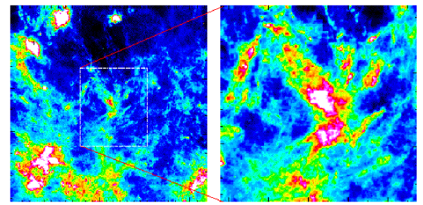
Figure 1: Left: IRAS 100 $\mu$m map of the Taurus molecular cloud complex, traced by the dust emission. The square is $\sim$ 4000 pc². Right Zoom of the central region (the square is now $\sim$ 400 pc²).

2.1 Low and High-mass Cut-off for the ISM Fractal

The largest self-gravitating entities in the Galaxy are the so-called Giant Molecular Clouds (or GMC) of about 100pc diameter, and 10⁶ M_⊙ in mass. Larger clouds cannot exist since they would be teared off by the galactic shear, i.e. the tidal forces due to the galactic potential itself. This is the high cut-off scale in the fractal structure. What is the smallest size?

It is difficult to observe directly in emission the smallest structure, due to lack of spatial resolution and sensitivity. But structures of about 10-20 AU in size (i.e. $\sim$ 10^-4 pc) have been observed for a long time through scattering of the quasar light (Fiedler et al. 1987, 1994, Fey et al. 1996): clumps in the electronic density diffract the light rays from remote quasars, and produce an ”extreme scattering event” (ESE) lasting for a few months, in their rapid motion (100-200km/s) just in front of the quasar. QSOs monitoring during several years has determined that the number of scattering structures is 10³ times as numerous as stars in the Galaxy. The problem of stability and life-time of these structures, with much higher pressure than surroundings, can be solved if they are self-gravitating (Walker & Wardle 1998); they are then of 10^-3 M_⊙ in mass, and have a gas density around 10¹⁰ cm^-3. They correspond to the smallest fragments predicted theoretically (Pfenniger & Combes 1994). These structures are now observed in a large number directly, through VLBI in the vicinity of the Sun, through HI absorption in front of quasars (e.g. Diamond e tal. 1989, Davis et al 1996, Faison et al 1998). If this 10-20 AU size is adopted for the low cut-off scale of the fractal structure, the latter ranges over 6 orders of magnitude in size, and about 10 in masses.

2.2 Scaling Laws

To better quantify the self-similar structure, several works have revealed that the interstellar clouds (either molecular or atomic) obey power-law relations between size, linewidth and mass (cf Larson 1981). These scaling relations are observed whatever the tracer. The original one is the size-linewidth relation (directly derived quantities), while the mass is only a secondary quantity, very uncertain to obtain, since there is no good universal tracer. The H₂ molecule does not radiate in the cold conditions of the bulk of the ISM (10-15 K), since it is symmetric, with no dipole moment. The first tracer is the most abundant molecule CO (10^-4 in number with respect to H₂), but it is most of the time optically thick, or photo-dissociated. The relation between the sizes $R$ and the line-widths or velocity dispersion $\sigma$, can be expressed through the power-law:

$$\sigma\propto R^{q}$$

with $q$ between 0.3 and 0.5 (e.g. Larson 1981, Scalo 1985, Solomon et al 1987, cf Fig. 2). There are some hints that molecular clouds are virialised (at least at large scale, since the masses are even more uncertain at low scales and high densities). If the virial is assumed at all scales, then:

$$\sigma^{2}\propto M/R$$

and the size-mass relation follows:

$$M\propto R^{D}$$

with $D$ the Hausdorff fractal dimension between 1.6 and 2. It can be deduced also that the mean density over a given scale R decreases as 1/R^α, where $\alpha$ is between 1 and 1.4.

Other interpretations are possible (see e.g. Falgarone 1998). Recently, Heithausen et al (1998) have extended the size-linewidth and size-mass relations down to Jupiter masses; their mass-size relation is M$\propto r^{2.31}$, much steeper than previous studies, but the estimation of masses at small scales is quite uncertain (in particular the conversion factor between CO and H₂ mass could be higher, and the mass at small-scale underestimated). It appears also that the self-similarity of structures is broken in regions of star formation. The break is observed as a change of slope in mass spectrum power laws at about 0.05pc in scale in the Taurus cloud, corresponding to the local Jeans length (Larson 1995). In other regions, either this break does not occur, or is occuring at larger scales (Blitz & Williams 1997, Goodman et al. 1998).

Dense gas is molecular, and cold H₂ molecules are difficult to trace (Combes & Pfenniger 1997). The tracer molecules such as CO are either optically thick, or not thermally excited (in low-density regions), photo-dissociated near ionizing stars, or depleted onto grains. Isotopic species, like ¹³CO or C¹⁸O, are poor tracers also, because of selective photo-dissociation. The large range of scales is also a source of bias, and of overestimates of the fractal dimension: the small scales are not resolved, and observed maps are smoothed out. This process, which makes the fractal look as a more diffuse medium of larger fractal dimension, can also lead to underestimates of the mass by factors more than 10 (e.g. simulations in Pfenniger & Combes 1994).

Figure 2: Top: Size-linewidth relation taken from various sources: Dam86: Dame et al. (1986); Sol87: Solomon et al. (1987); Heit98: Heithausen et al. (1998); MBM85: Magnani et al. (1985); Will94: Williams et al. (1994); Fal92: Falgarone et al. (1992); W95: Wang et al. (1995); Ward94: Ward-Thompson et al. (1994); Lem95: Lemme et al. (1995). An indicative line of slope 0.5 is drawn. Bottom: Mass-size relation deduced from the previous one, assuming that the structures are virialised. The line drawn has a slope of 2.

The observations of molecular clouds reveal that the structure is highly hierarchical, smaller clumps being embedded within the larger ones. This structure must be reminiscent of the formation mechanism, through recursive Jeans instability for instance. Since we have no real 3D picture, it is however difficult to ascertain a complete hierarchy, or to determine the importance of isolated clumps and/or a diffuse intercloud medium. An indicator of the 3rd dimension is the observed radial velocity, which is turbulent without systematic pattern. It has been possible, however, to build a tree structure where each clump has a parent for instance for clouds in Taurus (Houlahan & Scalo 1992).

2.3 2D-Projection of the Fractal

The projection of a fractal of dimension $D$ may not be a fractal, but if it is one with dimension $D_{p}$ it is impossible a priori to deduce its fractal dimension, except that

$D_{p}=D$ if $D\leq 2$

$D_{p}=2$ if $D\geq 2$ (Falconer 1990).

In 2D, the fractal dimension can be measured by computing the surface versus the perimeter of a given structure. This method has been used in observed 2D maps, like the IRAS continuum flux, or the extinctions maps of the sky. In all cases, this method converge towards the same fractal dimension $D_{2}$. For a curve of fractal dimension $D_{2}$ in a plane, the perimeter P and area A are related by

$$P\propto A^{D_{2}/2}$$

Falgarone et al (1991) find a dimension $D_{2}$ = 1.36 for CO contours both at very large (degrees) and very small scales (arcmin), and the same is found for IRAS 100$\mu$ contours in many circumstances (e.g. Bazell & Desert 1988). Comparable dimensions ($D_{2}$ between 1.3 and 1.5) are found with any tracer, for instance HI clouds (Vogelaar & Wakker 1994).

3 Turbulence

3.1 Theory

The interstellar medium is highly turbulent. To quantify, we can try to estimate the Reynolds number $R_{e}$, that separates the laminar (low $R_{e}$) from turbulent regimes:

$$R_{e}=vl/\nu$$

where $v$ is the velocity, $l$ a typical dimension, and $\nu$ the kinematic viscosity. Turbulent regimes are characterized by $R_{e}>>10^{3}$, implying that the advection term v . $\nabla$ v dominates the viscous term in the fluid equation. The turbulent state is characterised by unpredictable fluctuations in density and pressure, and a cascade of whirls. In the ISM, the viscosity can be estimated from the product of the macroturbulent velocity (or dispersion) and the mean-free-path of cloud-cloud collisions (since the molecular viscosity is negligible). But then the Reynolds number is huge ($\approx 10^{9}$), and the presence of turbulence is not a surprise.

This fact has encouraged many interpretations of the ISM structure in terms of what we know from incompressible turbulence. In particular, the Larson relations have been found as a sign of the Kolmogorov cascade (Kolmogorov 1941). In this picture, energy is dissipated into heat only at the lower scales, while it is injected only at large scale, and transferred all along the hierarchy of scales. Writing that the energy transfer rate $v^{2}/(r/v)$ is constant gives the relation

$$v\propto r^{1/3}$$

which is close to the observed scaling law, at least for the smallest cores (Myers 1983). The source of energy at large scale could be the differential galactic rotation and shear (Fleck 1981). This idealized view has been debated (e.g. Scalo 1987): it is not obvious that the energy cascades down without any dissipation in route (or injection), given the large-scale shocks, flows, winds, etc… observed in the ISM. The medium is highly supersonic (with Mach numbers larger then 10 in general), and therefore very dissipative. Energy could be provided at intermediate scale by stellar formation (bipolar flows, stellar winds, ionization fronts, supernovae..). Also, the interstellar medium is highly compressible, and its behaviour could be quite different from ordinary liquids in laboratory. However a modified notion of cascade could still be applied, leading to a Burgers spectrum, with

$$v\propto r^{1/2}$$

(see e.g. Vazquez-Semadeni et al. 1999).

The role of the magnetic field is still unclear. The intensity of the field has been measured through Zeeman line effects to be around a few $\mu$G in dense clouds (Troland et al. 1996, Crutcher et al 1999), and the observations are compatible with the hypothesis of equipartition between magnetic and kinetic energy. The magnetic field therefore plays an important role in energy exchange between the various degrees of freedom, but cannot prevent gravitational instabilities and cloud collapse, parallel to the field lines; although Gammie & Ostriker (1996) had found that magnetic waves could indeed provide some support in low dimensionality, in more realistic simulations there is almost no difference between $B=0$ and strongly magnetized models, as far as the dissipation and energy decay rates are concerned (Stone et al. 1998).

Besides, many features of ordinary turbulence are present in the ISM. For instance, Falgarone et al (1991) have pointed out that the existence of non-gaussian wings in molecular line profiles might be the signature of the intermittency of the velocity field in turbulent flows. More precisely, the ¹³CO average velocity profiles have often nearly exponential tails, as shown by the velocity derivatives in experiments of incompressible turbulence (Miesch & Scalo 1995). Comparisons with simulations of compressible gas give similar results (Falgarone et al 1994). Also the curves obtained through 2D slicing of turbulent flows have the same fractal properties as the 2D projected images of the ISM; their fractal dimension D₂ obtained from the perimeter-area relation is also 1.36 (Sreenivasan & Méneveau 1986).

More essential, the ISM is governed by strong fluctuations in density and velocity. It appears chaotic, since it obeys highly non-linear hydrodynamic equations, and there is coupling of phenomena at all scales. This is also related to the sensibility to initial conditions that defines a chaotic system. The chaos is not synonymous of random disorder, there is a remarquale ordering, which is reflected in the scaling laws. The self-similarity over several orders of magnitude in scale and mass means also that the correlation functions behave as power-laws, and that there is no finite correlation length. This characterizes critical media, experiencing a second order phase transition for example.

3.2 Turbulence Simulations

A large number of hydrodynamical simulations have been run, in order to reproduce the hierachical density structure of the interstellar medium. However, these are not yet conclusive, since the dynamical range available is still restricted, due to huge computational requirements. To gain in spatial resolution, 2D or even less (because of symmetries) computations are performed, but often the results cannot be generalised to 3D.

It has been argued that self-similar statistics alone can generate the observed structure of the ISM, in pressureless turbulent flows without self-gravity (Vazquez-Semadeni 1994); however, only three levels of hierarchical nesting can be traced. When heating and cooling processes are included, and since the corresponding time-scales are faster than the dynamical tine-scales, the gas can be derived by a polytropic equation of state, as $P\propto\rho^{\gamma}$, with $\gamma$ being the effective polytropic index. The isothermal value $\gamma$ = 1 is one of the possibilities, between 0 and 2 found in simulations.

From the size-linewidth relation $\sigma\propto R^{1/2}$, and the second observed scaling law $\rho\propto R^{-1}$, it can be deduced that

$$\sigma\propto\rho^{-1/2}$$

and therefore, if the turbulent pressure $P$ is defined as usual by

$$dP/d\rho=\sigma^{2}$$

it follows that

$$P\propto log\rho$$

which is the logatropic equation of state, or ”logatrope”. This behaviour has been tested in simulations (e.g. Vazquez-Semadeni et al 1998), but the logatrope has not been found adequate to represent dynamical processes occuring in the ISM (either hydro, or magnetic 2D simulations). The equation of state of the gas would be more similar to a polytrope of index $\gamma\approx 2$. But the results could depend whether the clouds are in approximate equilibrium or not (cf McLaughlin & Pudritz 1996).

Vazquez-Semadeni et al (1997) have searched for Larson relations in the results of 2D self-gravitating hydro (and MHD) simulations of turbulent ISM: they do not find clear relations, but instead a large range of sizes at a given density, and a large range of column densities; the Larson relation is more the upper envelope of the region occupied by simulated points in the $\rho$ - R diagram. They suggest that the observational results could be artefacts or selection effects (existence of a threshold in column density for UV-shielding for example).

MHD simulations have also explored the correlations between magnetic field strength and density, and field directions and filamentary morphology of clouds. Again, there is no clear correlation, only a larger scatter, with an upper envelope such as $B$ varying as $\rho^{0.4}$ (Padoan & Nordlund 1998, Padoan et al. 1998).

Note also that chemical reactions network, combined with turbulence, can be the source of considerable chaos (Rousseau et al. 1998).

4 Self-Gravity

4.1 Theory

Although the ISM is a self-organizing, multi-scale medium, comparable to what is found in laboratory turbulence, there are very special particularities that are not seen but in astrophysics. Self-gravity is a dominant, while it has not to be considered in atmospheric clouds for instance. It has been recognized by Larson (1981) and by many others that at each scale the kinetic energy associated with the linewidths balances the gravitational energy: clouds are virialized approximately, given their very irregular geometry.

Self-gravitating gas in an isothermal regime (which is a good approximation for the ISM), is known to be subject to instabilities. If we consider a sphere of gas confined in a box, and in contact with a thermostat, it will tend to follow an isothermal sphere, if the gas is hot enough. Below a certain critical temperature, there is no equilibrium any more, and the gas heats up when being cooled down, it is the gravothermal catastrophy, caused by negative specific heat (Lynden-Bell & Wood 1968). Small sub-condensations could form, and the physics will be more complex, since in the asymptotic case of an isolated clump, it will evaporate in a large number of dynamical times. The environment is quite important, and the fact that the clumps can exchange mass and energy with surroundings as well (e.g. Padmanabhan 1990).

Gravitational instability and cloud collapse is accompanied by fragmentation in a system with very efficient cooling, and this process can provide the turbulent motions observed. The theory was first proposed by Hoyle (1953) who showed that the isothermal collapse of a cloud led to recursive fragmentation, since the Jeans length decreases faster than the cloud radius. Rees (1976) has determined the size of the smallest fragments, when they become opaque to their own radiation. They correspond roughly to the smallest scales observed in the ISM (sizes of 10 AU, and masses of 10^-3 M_⊙, see the physical parameters of the ”clumpuscules” in Pfenniger & Combes 1994).

The hierarchical fractal structure yielded by recursive fragmentation can be simulated schematically, in order to estimate the resulting filling factor, and the biases introduced by observing with a limited spatial resolution (e.g. Pfenniger & Combes 1994). Clouds are distributed according to the radial distribution of an isothermal sphere in r^-2, and fragments also have positions selected randomly according to this radial distribution, and so on, hierarchically. The number $N$ of fragments at each level, and the fractal dimension $D$ chosen suffice to determine the size ratio between to imbricated spheres, i.e. = $N^{1/D}$. A sample of these fractals is shown in Fig. 3, for two dimensions 2.2 and 1.6.

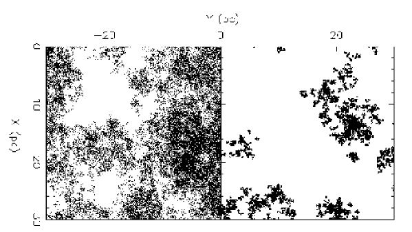
Figure 3: Left: Simulations of a fractal of dimension $D=2.2$ built by recursive fragmentation; Right: Same for a fractal of dimension $D=1.6$, the number of points are similar in the two cases.

Many other physical processes play a role in the turbulent ISM, as for instance rotation and magnetic fields. But they cannot be identified as the motor and the origin of the structure. Galactic rotation certainly injects energy at the largest scales, but angular momentum cannot cascade down the hierachy of clouds; indeed if the rotational velocity is too high, the structure is unstable to clump formation (cf Toomre criterium, 1964), and the non-axisymmetry evacuates angular momentum outside the structure. Magnetic fields are certainly enhanced by the turbulent motions, and could reach a certain degree of global equipartition with gravitational and kinetic energies in tbe virialised clouds. But they cannot be alone at the origin of the hierarchical structure, gravity has to trigger the collapse first. Besides, there is no observational evidence of the gas collapse along the field lines, polarisation measurements give contradictory results for the field orientation with respect to the gas filaments. Therefore, although rotation, turbulence, magnetic fields play an important role in the ISM, they are more likely to be consequences of the formation of the structure.

4.2 Self-gravitating Simulations

Simulations of self-gravitating gas are very demanding, since large gradients rapidly set up, and spatial resolution must be adapted. A general rule is that the resolution is well below the Jeans length at any point, but the Jeans length shrinks along the collapse. Artificial fragmentation can sometimes happen due to artifacts (see e.g. Truelove et al. 1997). To compensate for the limited spatial range, periodic boundary conditions are used, to simulate the ISM. Klessen (1997) and Klessen et al. (1998) have considered the fragmentation of molecular clouds, in 3D, starting with an homogenous cloud with small primordial fluctuations. These initial conditions are very similar to what is used in a cosmological background. The fluctuations are a gaussian density field with power spectrum P(k) $\propto$ k^-2. After one free-fall time, the gas has evolved into a system of filaments and knots, some of them contain collapsing cores. To avoid the problem of spatial resolution, the condensed cores are then replaced by sink particles, simulating therefore a low cut-off scale.

Klessen et al. (1998) compute the mass spectrum of clumps, which looks very similar to the observed one $dN/dm\propto m^{-1.5}$ in the ISM, at least over 1.5 order of magnitude. The results however, depends still a lot on the initial conditions, and the power spectrum used (Semelin & Combes 1999). One of the problem of these simulations, in comparison with the ISM, is the absence of energy re-injection, and systematic motions. In a Galaxy, differential rotation and shear should provide both.

Taking into Account the Shear

One way to re-inject energy at large scale is the differential rotation of the Galaxy, as we have already emphasized. Computations of self-gravitating shearing sheets have already given interesting large-scale structures, that might be similar ro fractals. Toomre (1990) carried out self-gravitating simulations on gas particles, that were regularly cooled, in a shearing environment, and a quasi-periodical boundary conditions. In fact, the periodicity has to take into account the shear motions, and proper sliding of the sheet at larger and smaller radii is necessary in order to ensure continuity. The main result is a steady wave pattern, that sets quickly in through gravitational instabilities, and differential rotation, and is continuously renewed. Toomre (1990) was surprised himself of the efficiency of the mechanism, and of its quasi-stationarity: the energy dissipated in the gas cooling was compensated exactly by the rotational shear. This could be the main energy source was the gravitational structures in the ISM of galaxies. Toomre & Kalnajs (1994) refined the computations, and obtained the ”typical” morphology of the pattern. These simulations demonstrate the power of gravity, allied with shear, to produce spiral structure, by the swing mechanism. They also show how much structures at all scales, or spiral chaos, can be sustained and maintained by the self-gravitation of a cooled granular distribution.

The work was taken up recently by Huber & Pfenniger (1999), that generalised the computations in 3D, taking into account the galaxy plane thickness of the gaseous component. Their cooling is simulated by a viscous force, proportional to the particle velocity. They also find the characteristic filaments due to the shear combined with self-gravity, and measure the corresponding fractal dimension of the structures. Since the filaments are much longer in the plane than thick (perpendicular to it), the fractal dimension is in fact dominated by the z-dimension plane morphology, at least at large scales. So the range of scale where the fractal dimension is lower than 2 is very small. The boarder effects are then too large to determine $D$ without ambiguity. These calculations are however encouraging that a fractal structure could develop at sub-kpc scales, when shearing is dominant, near the high cut-off of the ISM fractal.

In a recent work (Semelin & Combes, 1999), we have also tried to determine the fractal dimension of a nearly isothermal self-gravitating gas. A tree-code and cloud-cloud collisions algorithm was used in 2D and 3D to follow the collapse of a periodically-replicated piece of ISM. Without shear, the collapse of initial perturbations are followed , and a fractal structure is found only in a transient way. With energy re-injection, and in particular with shear (and Coriolis forces), the structures are formed over several orders of magnitude. The characteristic spiral filaments are observed, and embedded clumps form, and can disappear and reform stochastically. Simulations of a shearing sheet are shown in Fig 4. The fractal dimension derived is around 1.8.

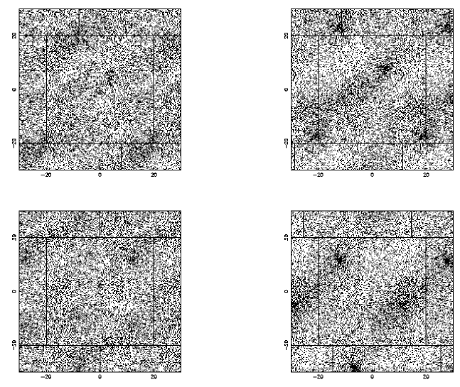
Figure 4: From Left to Right, and Top to Bottom: Simulations in 2D of a shearing sheet of gas particles, subject to their own self-gravity, and to collisions (dissipation). The central square in each frame is the area simulated, and the lanes surrounding it have been plotted to show the particular periodicity, that takes into account the shear (relative X-motions). The gradient of the rotational angular velocity $\Omega$ is along the Y-axis. The time is 1, 4, 11, and 16 free-fall times respectively for the four successive frames.

Wada & Norman (1999) have also simulated a shearing galaxy disk, but with a multi-phase medium: they obtain the formation of dense clumps and filaments, surrounded by a hot diffuse medium. The quasi-stationary filamentary structure of the cold gas is another manifestation of the combination of shear and self-gravity in a cooled gas.

5 Galaxy Distributions

It has been known for a long time that galaxies are not distributed homogeneously in the sky, but they follow a hierarchical structure: galaxies gather in groups, that are embedded in clusters, then in superclusters, and so on (Charlier 1908, 1922, Shapley 1934, Abell 1958). Moreover, galaxies and clusters appear to obey scaling properties, such as the power-law of the two point-correlation function:

$$\xi(r)\propto r^{-\gamma}$$

with the slope $\gamma$, the same for galaxies and clusters, of $\approx$ 1.7 (e.g. Peebles, 1980, 1993). According to the self-similar morphology, and the scaling laws, the galaxy ensemble can also be characterized by a fractal. But what are the limiting scales?

5.1 Low and High-mass cut-off for the galaxies fractal

The smallest structure is of course a galaxy, and the starting point of the fractal is therefore obvious: 10 kpc in scale, and about 10¹⁰ M_⊙, representative of a dwarf galaxy. The high-mass cut-off is much less obvious, and there has been a continuous debate in the recent years to know what is the scale of transition to homogeneity, and even whether this scale exists.

Isotropy and homogeneity are expected at very large scales from the Cosmological Principle (e.g. Peebles 1993). The main observational evidence in favor of the Cosmological Principle is the remarkable isotropy of the cosmic background radiation (e.g. Smoot et al 1992), that provides information about the Universe at the matter/radiation decoupling. At very large scales, the Universe must then be homogeneous. There must exist a transition between the small-scale fractality to large-scale homogeneity. This transition is certainly smooth, and might correspond to the transition from linear perturbations to the non-linear gravitational collapse of structures. The present catalogs do not yet see the transition since they do not look up sufficiently back in time. It can be noticed that some recent surveys begin to see a different power-law behavior at large scales ($\lambda\approx 200-400h^{-1}$ Mpc, e.g. Lin et al 1996, Scaramella et al. 1998). The interpretation depends however on the K-correction adopted, and the curvature of the Universe (Joyce et al. 1999).

Summarizing, it appears that the high-mass cut-off could be at the present epoch at about 300 Mpc and 10¹⁷ M_⊙, the mass of the largest superclusters. The fractal extends over about 4 orders of magnitude is scale and 7 in mass. It is smaller than the ISM fractal, but since larger and larger structures could decouple from inflation and develop, this range could still increase.

5.2 Correlation Function and Conditional Density

The debate on the spatial extent of the fractal has been complexified by the use of the correlation function to quantify the scaling laws in galaxy distributions. The correlation function is defined as

$$\xi(r)=\frac{<n(r_{i}).n(r_{i}+r)>}{<n>^{2}}-1$$

where $n(r)$ is the number density of galaxies, and $<...>$ is the volume average (over $d^{3}r_{i}$). One can always define a correlation length $r_{0}$ by $\xi(r_{0})=1$.

This definition involves the average density $<n>$, which depends on the scale for a fractal distribution. This is unfortunate, since the derived correlation parameters (slope and correlation lengths) then depend on the galaxy sample used (see Davis 1997, Davis et al 1988, Pietronero et al 1997). The fact that there exists a correlation length does not mean that there is no fractal, because of its definition different from that used in physics; there $\xi_{0}$ characterizes the exponential decay of correlations $(\sim e^{-r/\xi_{0}})$ (for power decaying correlations, the correlation length is infinite). Davis & Peebles (1983) or Hamilton (1993) argue that the fractal of galaxies cannot have a large spatial extent, since the galaxy-galaxy correlation length $r_{0}$ is rather small. The most frequently reported value is $r_{0}\approx 5h^{-1}$ Mpc (where $h=H_{0}$/100km s^-1Mpc^-1).

The same problem occurs for the two-point correlation function of galaxy clusters; the corresponding $\xi(r)$ has the same power law as galaxies, their length $r_{0}$ has been reported to be about $r_{0}\approx 25h^{-1}$ Mpc, and their correlation amplitude is therefore about 15 times higher than that of galaxies (Postman, Geller & Huchra 1986, Postman, Huchra & Geller 1992). The latter is difficult to understand, unless there is a considerable difference between galaxies belonging to clusters and field galaxies (or morphological segregation). The other obvious explanation is that the normalizing average density of the universe was then chosen lower.

Assuming that the average density is a constant, while homogeneity is not yet reached, could perturb significantly the correlation function, and its slope, as shown by Coleman, Pietronero & Sanders (1988) and Coleman & Pietronero (1992). The function $\xi(r)$ has a power-law behaviour of slope $-\gamma$ for $r<r_{0}$, then it turns down to zero rather quickly at the statitistical limit of the sample. This rapid fall leads to an over-estimate of the small-scale $\gamma$. Pietronero (1987) introduces the conditional density

$$\Gamma(r)=\frac{<n(r_{i}).n(r_{i}+r)>}{<n>}$$

which is the average density around an occupied point. For a fractal medium, where the mass depends on the size as $M(r)\propto r^{D}$, $D$ being the fractal (Haussdorf) dimension, the conditional density behaves as $\Gamma(r)\propto r^{D-3}$.

It is possible to retrieve the correlation function as

$$\xi(r)=\frac{\Gamma(r)}{<n>}-1$$

In the general use of $\xi(r)$, $<n>$ is taken for a constant, and we can see that

$$D=3-\gamma\quad.$$

If for very small scales, both $\xi(r)$ and $\Gamma(r)$ have the same power-law behaviour, with the same slope $-\gamma$, then the slope appears to steepen for $\xi(r)$ when approaching the length $r_{0}$. This explains why with a correct statistical analysis (Di Nella et al 1996, Sylos Labini & Amendola 1996, Sylos Labini et al 1996), the actual $\gamma\approx 1-1.5$ is smaller than that obtained using $\xi(r)$ (cf Fig. 5). This also explains why the amplitude of $\xi(r)$ and $r_{0}$ increases with the sample size, and for clusters as well.

Figure 5: Bottom: the average conditional density $\Gamma(r)$ for several samples (Perseus-Pisces and CfA1 in open rectangles, and LEDA in filled triangles, adapted from Sylos-Labini & Pietronero 1996). Top: $\xi(r)$ corresponding to the same surveys. The indicative line has a slope $\gamma=1$ (corresponding to a fractal dimension $D\sim 2$). This shows that it is difficult to determine the slope on the $\xi(r)$ function.

Note that the fractal distribution in the galaxy catalogs has been determined from the light distribution, and this could be somewhat different from the mass distribution. There is also a morphological segregation of galaxies in clusters, and the different types of galaxies (ellipticals, spirals, or dwarfs) do not trace the same distribution. The mass distribution could be more complex. All this has led to the introduction of multifractality to represent the Universe (e.g. Sylos-Labini & Pietronero 1996). In a multifractal system, local scaling properties slightly evolve, and can be defined by a continuous distribution of exponents. This is a mere generalisation of a simple fractal, that links the space and mass distributions. Mutlifractality may also better account for the transition to homogeneity, with a fractal dimension varying with scale (Balian & Schaeffer 1989, Castagnoli & Provenzale 1991, Martinez et al 1993, Dubrulle & Lachièze-Rey 1994).

5.3 Definition of the Self-Gravity Domain

The general view in cosmologiacl models is that the galaxy structures in the Universe have developped by gravitational collapse from primordial fluctuations. Once unstable, density fluctuations do not grow as fast as we are used to for Jeans instability (exponential), since they are slowed down by expansion. The rate of growth is instead a power-law, in the linear regime. If $\delta$ is the density contrast:

$$\delta(\vec{x})=(\rho(\vec{x})-<\rho>)/<\rho>$$

where $<\rho>$ is the mean density of the Universe, assumed homogeneous at very large scale. If $\vec{r}$ is the physical coordinate, the comoving coordinate $\vec{x}$ is defined by $\vec{r}=a(t)\vec{x}$, where a(t) is the scale factor, accounting for the Hubble expansion (normalised to a(t₀) = 1 at the present time). Since the Hubble constant verifies $H(t)=\dot{a}/a$, the peculiar velocity is defined by

$$\vec{v}=\dot{\vec{r}}-H\vec{r}=a\dot{\vec{x}}$$

In comoving coordinates, the Poisson equation becomes:

$$\nabla_{x}^{2}\Phi=4\pi Ga^{2}(\rho-<\rho>)$$

It can be shown easily that in a flat universe, the density contrast in the linear regime grows as the scale factor $a(t)=(t/t_{0})^{2/3}$. In the non-linear regime, on the contrary, the density $\rho$ is much larger with respect to $<\rho>$, and the normal self-gravity and Jeans instability is retrieved. The receding velocities due to inflation do not exist anymore. The structures are bound and decoupled from inflation. It is natural to define the self-gravity domain as limited by the largest decoupled structures, and if self-gravity is responsible for the fractal structure, it is expected that this scale will also delimit the transition to homogeneity.

6 Statistical Mechanics of Self-Gravity

Both for the ISM and for galaxy distributions in the Universe, self-similar structures are observed over large ranges in scales. Scaling laws are observed, which translate by an average density decreasing with scale as a power-law, of slope $-\gamma$ between -1.5 and -1, corresponding to a fractal dimension $D=3-\gamma$ between 1.5 and 2. In the following, we will investigate the hypothesis that the main driver responsible for these fractal structures is self-gravity, even though the actual structures migh be more complex and perturbed.

Since gravity is scale-independent, there are opportunities for a mechanism to propagate over scales in a self-similar fashion. For the ISM, in a quasi isothermal regime, a fractal structure could be build through recursive Jeans instability and fragmentation. This recursive fragmentation proceeds until the density is high enough to reach the adiabatic regime. Self-gravity could be the principal origin of the fractal, with generated turbulent motions in virial equilibrium at each scale. For galaxy formation, the smallest structures collapse first, and these influence the largest scale in a non-linear manner. It is obvious that in both cases, the system does not tend to a stationary point, but develops fluctuations at all scales, and these must be studied statistically.

Recently, de Vega, Sanchez & Combes (1996a,b, 1998) have proposed a statistical field theory of self-gravity, not only to account for the existence of the structure, but also to be able to predict its fractal dimension and others critical exponents. This has been obtained by developping the grand partition function of the ensemble of self-gravitating particles. In transforming the partition function through a functional integral, it can be shown that the system is exactly equivalent to a scalar field theory. The theory does not diverge, since the system is considered only between two scale limits: the short-scale and large-scale cut-offs. Through a perturbative approach it can be demonstrated that the system has a critical behaviour, for any parameter (effective temperature and density). That is, we can consider the self-gravitating gaseous medium as correlated at any scale, as for the critical points phenomena in phase transitions (as was first suggested by Totsuji & Kihara 1969).

Note that this approach is quite different from the thermodynamical approach developped by Saslaw & Hamilton (1984). Their theory is based on the thermodynamics of gravitating systems, which assumes quasi thermodynamic equilibrium. They justified this equilibrium at the small-scales of non-linear clustering, because the local relaxation and dynamical time-scales are much shorter than the expansion time-scale. The theory considers the essential parameter $b(t)$, the ratio of gravitational correlation energy to thermal kinetic energy, and deduces the value of this parameter from the observations. It appears that $b(t)$ varies also with scale. The predictions of the thermodynamical theory have been successfully compared with N-body simulations (Itoh et al. 1993, Sheth & Saslaw 1996, Saslaw & Fang 1996).

6.1 Hamiltonian of the Self-Gravitating Ensemble of N-bodies

Let us consider a gas of particles submitted only to their self-gravity, in thermal equilibrium at temperature T $(kT=\beta^{-1})$. In the interstellar medium, quasi isothermality is justified, due to the very efficient cooling. For unperturbed gas in the outer parts of galaxies, gas is in equilibrium with the cosmic background radiation at $T\approx 3K$ (Pfenniger et al 1994, Pfenniger & Combes 1994). For a system of collapsing structures in the universe, this can be a valid approximation, as soon as the gradient of temperature is small over a given scale.

This isothermal character is essential for the description of the gravitational systems as critical systems, as will be shown later, so that the canonical ensemble appears the best adapted system. Moreover, the systems considered are not isolated gravitational systems, for which the microcanonical system should be used (e.g. Horwitz & Katz 1978a,b; Padmanabhan 1990). On the contrary, the mass or number of particles is not fixed, and according to the fluctuations, matter can enter any given scale, through condensation or evaporation. The best statistical frame to consider is then the grand canonical ensemble, allowing for a variable number of particles $N$. The grand partition function ${\cal Z}$ and the Hamiltonian $H_{N}$ are

$${\cal Z}=\sum_{N=0}^{\infty}\;{{z^{N}}\over{N!}}\;\int\ldots\int\prod_{l=1}^{N}\;{{d^{3}p_{l}\,d^{3}q_{l}}\over{h^{3}}}\;e^{-\beta H_{N}}$$

$$H_{N}=\sum_{l=1}^{N}\;{{p_{l}^{2}}\over{2m}}-G\,m^{2}\sum_{1\leq l<j\leq N}{1\over{|{\vec{q}}_{l}-{\vec{q}}_{j}|}}$$

where $z$ is the fugacity = $exp(-\beta\mu_{c})$ in terms of the gravito-chemical potential $\mu_{c}$, and $h$ is now the Planck constant.

The latter integral can be transformed, using the continuous density $\rho({\vec{r}})=\sum_{j=1}^{N}\;\delta({\vec{r}}-{\vec{q}}_{j})\;$ and integrated to yield the potential, but introducing a cutoff $a$ for the minimum separation between particles, so that there is no problem of divergence. The cutoff $a$ is here introduced naturally, it corresponds to the size of the smallest fragments, or clumpuscules (of the order of $\sim 10$ AU). In fact, we consider that the particles of the system interact with the Newton law of gravity ($1/r$) only within the size range of the fractal, where self-gravity is predominant. At small scale, other forces enter into account, and we can adopt a model of hard spheres to schematize them. Also at large scales, beyond the upper cutoff, different forces must be introduced. The phenomenological potential thus considered does not possess any singularity.

6.2 ${\cal Z}$ as the Partition Function of a Single Scalar Field $\phi$

Using the potential in $1/r$, and its inverse operator $-\frac{1}{4\pi}\nabla^{2}$ (but see also a similar derivation, with $[1-\theta(a-r)]/r$ and its corresponding inverse operator, for the phenomenological potential with cutoff, in de Vega et al 1996b), the exponent of the potential energy can be represented as a functional integral (Stratonovich 1958, Hubbard 1959)

$$e^{\frac{1}{2}\,\beta G\,m^{2}\int\;{{d^{3}x\,d^{3}y}\over{|{\vec{x}}-{\vec{y}}|}}\;\rho({\vec{x}})\rho({\vec{y}})}=\int\int\;{\cal D}\xi\;e^{-\frac{1}{2}\int d^{3}x\;(\nabla\xi)^{2}\;+\;2m\sqrt{\pi G\beta}\;\int d^{3}x\;\xi({\vec{x}})\;\rho({\vec{x}})}$$

With the change of variables: $\phi({\vec{x}})\equiv 2m\sqrt{\pi G\beta}\;\xi({\vec{x}})$ and

$$\mu^{2}={{\pi^{5/2}}\over{h^{3}}}\;z\;G\,(2m)^{7/2}\,\sqrt{kT}\;\quad,\quad T_{eff}=4\pi\;{{G\;m^{2}}\over{kT}}\quad$$

the partition function can be written as a functional integral ${\cal Z}=\int\int\;{\cal D}\phi\;e^{-S}$ where the action $S$ is:

$$S[\phi(.)]\equiv{1\over{T_{eff}}}\;\int d^{3}x\left[\frac{1}{2}(\nabla\phi)^{2}\;-\mu^{2}\;e^{\phi({\vec{x}})}\right]$$

Note that the ”equivalent” temperature $T_{eff}$ in the field theory is in fact inversely proportional to the physical temperature. It can be shown that the parameter $\mu$ is equal to the inverse of the Jeans length, itself of the order of the cutoff $a$.

It is then possible to compute the statistical average of physical quantitites, such as the density $\rho({\vec{r}})$

$$<\rho({\vec{r}})>=-{1\over{T_{eff}}}\;<\nabla^{2}\phi({\vec{r}})>={{\mu^{2}}\over{T_{eff}}}\;<e^{\phi({\vec{r}})}>$$

where $<\ldots>$ means functional average over $\phi(.)$ with statistical weight $e^{S[\phi(.)]}$.

The equation for stationary points: $\nabla^{2}\phi=-\mu^{2}\,e^{\phi({\vec{x}})}\;$ has two main solutions. One is the constant stationary solution: $\phi_{0}=-\infty$; and the second is the singular isothermal sphere: $\phi(r)=\log{{2}\over{\mu^{2}r^{2}}}$. With a perturbative method, starting from the stationary solution $\phi_{0}=-\infty$, it has been shown that the theory scales, at large distances (de Vega et al 1996b). The same has been shown, starting from the isothermal sphere solution (Semelin et al. 1998). In the latter case, the development in series of the density correlation function is made with the relevant effective coupling constant:

$$\lambda={{T_{eff}}\over{R}}$$

and this coupling constant evolves through the renormalisation group equations with the scale $R$, or scale ratio $\tau=ln(R/a)$, where $a$ is the low cut-off scale. A remarkable behaviour is found for $\lambda(\tau)$, since it vanishes periodically, for values $\tau_{n}$ = $2\pi n/\sqrt{7}$ ($n$ integer). Periodically, the coupling constant diverges to infinity, which means that the perturbation theory is no longer valid, because of strong coupling. This occurs for scales:

$$R_{n}=R_{0}e^{2\pi n/\sqrt{7}}=R_{0}(10.749)^{n}$$

It appears then a hierachy of scale, varying by about an order of magnitude at each level. This numerical factor 10.749 depends essentially on the spherical geometry assumed for the computations, but is expected to be different for different geometries (like filaments, for example).

7 Renormalization Group Methods

The renormalization methods are very powerful to deal with self-similar systems obeying scaling laws, like critical phenomena. In the latter case, examplified by second order phase transitions, there exist critical divergences, where physical quantities become singular as power-laws of parameters called critical exponents. These critical systems reveal a collective behaviour, organized from microscopic degrees of freedom, through giant fluctuations and statistical correlations. Hierarchical structures are built up, coupling all scales together, replacing an homogeneous system in a scale-invariant system. It can be shown that local forces are not important to describe the collective behaviour, which is only due to the statistical coupling of local interactions. Therefore, critical exponents depend only on the statistical distribution of microscopic configurations, i.e. on the dimensionalities or symmetries of the system. There exist wide universality classes, that allow to draw quantitative predictions on the system from only a qualitative knowledge of its properties (e.g. Parisi, 1988; Zinn-Justin 1989; Binney et al 1992).

7.1 Critical Phenomena

Critical phenomena occur at second order phase transitions, i.e. continuous transitions without latent heat. The paradigm of these systems is the transition at the Curie point (T=T_c= 1043K) from paramagnetic iron, where the magnetic moment is proportional to the applied field m=$\mu$ B, to ferromagnetic state, where there exists a permanent magnetic moment m₀ even in zero field. Although the permanent magnet tends to zero continuously at T_c, there are divergences: for instance the heat capacity C behaves as C$\propto|T-T_{c}|^{-\alpha}$, with $\alpha>0$.

Also for the critical point of water, at which the transition from the liquid to gas becomes continuous, the compressibility $\kappa_{T}\propto|T-T_{c}|^{-\gamma}$. At the critical point, it is easy to understand that the compressibility which tends to infinity generates large density fluctuations, and therefore light is strongly diffused by the varying optical index: this is the critical opalescence. The extraordinary fact is that microscopic forces can give rise to large-scale fluctuations, as if the medium was organized at all scales (cf Fig. 6).

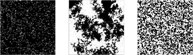
Figure 6: Illustration of the fractal structure occuring when a Ising system passes through the critical temperature (a second order phase transition). The temperature is near zero at left, about critical in the center, and much larger than critical at right (from a simulation of the Ising model with a Monte-Carlo method)

7.2 Universality of Critical Exponents

Experiments have shown that the critical exponents for a wide variety of systems are the same, and more precisely they belong to universality classes, depending only on the dimensionality $d$ of space and $D$ of the order parameter (for instance if the field is scalar or a vector with dimension $D$). This universality means that the details of the local forces are unimportant; therefore the local interactions can be simply modelled, through a schematic hamiltonian supposed to hold the relevant symmetries of the system. There exists only 2 independent critical exponents.

Renormalization techniques were applied to statistical physics in the 1970s (Wilson & Kogut 1974; Wilson 1975, 1983). In a renormalization group transformation, the scales are divided by a certain factor $k$, and particles are replaced by a block of particles. Since the system is scale-independent, it should be possible to find an hamiltonian for the blocks which is of the same structure as the original one. The new system is less critical than the previous one, since the correlation length $\xi$ has also been divided by $k$. It is a way to reduce the number of degrees of freedom of the system. With these techniques, precise values of the critical exponents have been computed, for a whole range of models, and can be used for any problem in the same universality class.

7.3 Statistical Self-Gravity

As was shown in section 6, the grand-canonical self-gravitating system is critical for a large range of the parameters, and it is difficult to isolate a critical point, to identify diverging behaviours. However, it is well known (Wilson 1975, Domb & Green 1976), that physical quantities diverge only for infinite volume systems, at the critical point. Since the self-gravitating systems are also finite and bounded, they only approach asymptotically the divergences.

If $\Lambda$ measures the distance to the critical point, (in spin systems for instance, $\Lambda$ is proportional to $|T-T_{c}|$), the correlation length $\xi$ diverges like

$$\xi(\Lambda)\sim\Lambda^{-\nu}\;$$

and the specific heat (per unit volume) as ${\cal C}\sim\Lambda^{-\alpha}\;$. But in fact, for a finite volume system, all physical quantities are finite at the critical point. When the typical size $R$ of the system is large, the physical magnitudes take large values at the critical point, and the infinite volume theory is used to treat finite size systems at criticality. In particular, for our system, the correlation length provides the relevant physical length $\xi\sim R$, and we can write

$$\Lambda\sim R^{-1/\nu}\;$$

The self-gravitating systems considered here have the symmetries $d=3$ and $D=1$ (scalar field), which should indicate the universality class to which it corresponds. It remains to identify the corresponding operators. Already in the previous sections, it was suggested that the field $\phi$ corresponds to the potential, and the mass density

$$m\,\rho({\vec{x}})=m\,\,e^{\phi({\vec{x}})}$$

can be identified with the energy density in the renormalization group (also called the ‘thermal perturbation operator’).

We note that the state of zero density (or zero fugacity), corresponds to a singular point, around which we develop the physical functions (and we choose $\Lambda$ accordingly). At this point $\mu^{2}/T_{eff}=0$, the partition function ${\cal Z}$ is singular

$$\Lambda\equiv{{\mu^{2}}\over{T_{eff}}}=z\,\left({{2\pi mkT}\over{h^{2}}}\right)^{3/2}\;$$

i.e., the critical point $\Lambda=0$ corresponds to zero fugacity $z$. Writing ${\cal Z}$ as a function of the action $S^{*}$ at the critical point

$${\cal Z}(\Lambda)=\int\int\;{\cal D}\phi\;e^{-S^{*}+\Lambda\int d^{3}x\;e^{\phi({\vec{x}})}\;}$$

and computing statistical averages (de Vega et al. 1996a,b), the mass fluctuations and corresponding dispersion can be found as:

$$(\Delta M(R))^{2}\equiv\;<M^{2}>-<M>^{2}\sim\int d^{3}x\;d^{3}y\;C({\vec{x}},{\vec{y}})\sim R^{2/\nu}$$

$$\Delta M(R)\sim R^{1/\nu}$$

This is the definition relation of the fractal, with dimension $d_{H}$, and the scaling exponent $\nu$ can be identified with the inverse Haussdorf dimension of the system, $d_{H}=\frac{1}{\nu}$. The velocity dispersion follows: $\Delta v\sim R^{q}$, with $q=\frac{1}{2}\left(\frac{1}{\nu}-1\right)=\frac{1}{2}(d_{H}-1)$.

The scaling exponents $\nu,\;\alpha$ have been computed through the renormalization group approach. The case of a single component (scalar) field has been extensively studied in the literature (Hasenfratz & Hasenfratz 1986, Morris 1994a,b). For the Ising model $d=3$, the exponent $\nu$ = 0.631, from which we deduce $d_{H}$ = 1.585. Alternatively, in the case of weak perturbations, the mean field theory can be applied, and $d_{H}$ = 2. These values are compatible with the observed ones for astrophysical fractals.

8 Conclusion

We have emphasized the existence of two astrophysical fractals, the interstellar medium, with structures ranging from 10 AU to 100 pc, and the large-scale structures of galaxies, from 10 kpc to 200 Mpc at least. The first one is in statistical equilibrium, while the second one is still growing to larger scales. In both cases, we can describe these media as developping large-scale fluctuations with large correlations as is familiar in critical phenomena. We have investigated the hypothesis that in both cases, self-gravity is the main force governing these fractal structures.

Numerical simulations can help to understand the formation of these structures, and the main mechanisms at play. Unfortunately, practical constraints confine the possibilities to a limited range of scales, and results are often ambiguous. Simulations of MHD turbulence with self-gravity are not yet to the point to reproduce the scaling relations observed in the ISM. Purely self-gravitating simulations without large-scale injection of energy produce only transient fractal structures, depending in a large part on initial conditions. When large-scale energy is taken into account (by the galaxy shear namely), a quasi-stationary fractal structure, over $\sim$ two orders of magnitudes, can be obtained. This is encouraging, waiting for more performant 3D simulations.

A statistical thermodynamic approach of self-gravitating systems has been developped, and it is shown that the phenomenological potential, which is in $1/r$ between two cutoffs (at small and large-scale), can be described by a scalar field theory. Using renormalization group methods, the system is found to be of the same universality class as the Ising $d=3$ model. The critical exponents can then be derived, and the fractal dimension $D=1.6$ deduced.

The gravitational gas appears to be critical for a large range of temperatures and couplings, while for spin models there is only a critical value of the temperature. This feature must be connected with the scale invariant character of the Newtonian force and its infinite range.

References

- [1] Abell G.O.: 1958, ApJS 3, 211
- [2] Balian R., Schaeffer R.: 1989, A&A 226, 373
- [3] Bazell D., Desert F.X.: 1988, ApJ 333, 353
- [4] Binney J.J., Dowrick N.J., Fisher A.J., Newman M.E.J.: 1992 ‘The Theory of Critical Phenomena’, Oxford Science Publication.
- [5] Blitz, L., Williams J.P.: 1997 ApJ 488, L145
- [6] Castagnoli C., Provenzale A.: 1991, A&A 246, 634
- [7] Charlier C.V.L., 1908, Arkiv för Mat. Astron. Fys. 4, 1
- [8] Charlier C.V.L., 1922, Arkiv för Mat. Astron. Fys. 16, 1
- [9] Coleman P.H., Pietronero L., Sanders R.H.: 1988, A&A 200, L32
- [10] Coleman P.H., Pietronero L.: 1992, Phys. Rep. 231, 311
- [11] Combes F., Pfenniger D.: 1997, A&A 327 453
- [12] Crutcher, R. M., Troland, T. H., Lazareff, B., Paubert, G., Kazès, I.: 1999 ApJ 514, L121
- [13] Dame T.M., Elmegreen B.G., Cohen R.S., Thaddeus P.: 1986, ApJ 305, 982
- [14] Dame T.M., Hartmann D., Thaddeus P., 1996 BAAS 189, 7004
- [15] Davis M.A., Meiksin M.A., Strauss L.N., da Costa and Yahil A.: 1988, ApJ 333, L9
- [16] Davis M.A.: 1997 in ‘Critical Dialogs in Cosmology’, ed. N. Turok, astro-ph/9610149
- [17] Davis M.A., Peebles P.J.E.: 1983, ApJ 267, 465
- [18] Davis R.J., Diamond P.J., Goss W.M.: 1996, MNRAS 283, 1105
- [19] de Vega H., Sánchez N., Combes F.: 1996a, Nature 383, 53
- [20] de Vega H., Sánchez N., Combes F.: 1996b, Phys. Rev. D54, 6008
- [21] de Vega H., Sánchez N., Combes F.: 1998, ApJ in press
- [22] Diamond P.J., Goss W.M., Romney J.D. et al: 1989, ApJ 347, 302
- [23] Di Nella H., Montuori M., Paturel G., Pietronero L., Sylos Labini F.: 1996, A&A 308, L33
- [24] Domb C., Green M.S.: 1976, ‘Phase transitions and Critical Phenomena’, vol. 6, Academic Press
- [25] Dubrulle B., Lachièze-Rey M.: 1994, A&A 289, 667
- [26] Faison M.D., Goss W.M., Diamond P.J., Taylor G.B., 1998, AJ 116, 2916
- [27] Falconer K.J.:1990, Fractal geometry, Wiley, Chichester
- [28] Falgarone, E., Phillips, T.G., Walker, C.K.: 1991, ApJ 378, 186
- [29] Falgarone, E., Puget J-L., Perault M., 1992, A&A 257, 715
- [30] Falgarone, E., Lis D.C., Phillips, T.G. et al: 1994, ApJ 436, 728
- [31] Falgarone E., 1998, in “Starbursts: triggers, nature and evolution”, Les Houches Summer School, ed. B. Guiderdoni, A. Kembhavi, Springer, p. 41
- [32] Fey A.L., Clegg A.W., Fiedler R.L., 1996, ApJ 468, 543
- [33] Fiedler R.L., Dennison B., Johnston K., Hewish A.: 1987, Nature 326, 675
- [34] Fiedler R.L., Pauls T., Johnston K., Dennison B.: 1994, ApJ 430, 595
- [35] Fleck R.C.: 1981, ApJ 246, L151
- [36] Gammie C.F., Ostriker E.C.: 1996, ApJ 466, 814
- [37] Goodman, A. A., Barranco, J. A., Wilner, D. J., Heyer, M. H.: 1998, ApJ 504, 223
- [38] Hamilton A.J.S.: 1993, ApJ 417, 19
- [39] Hasenfratz A., Hasenfratz P., 1986, Nucl.Phys. B270, 687
- [40] Heithausen A., Bensch F., Stutzki J., Fakgarone E., Panis J.F.: 1998, A&A 331, L65
- [41] Horwitz G., Katz J., 1978a, ApJ 222, 941
- [42] Horwitz G., Katz J., 1978b, ApJ 223, 311
- [43] Houlahan P., Scalo J.: 1992, ApJ 393, 172
- [44] Hoyle F.: 1953, ApJ 118 513
- [45] Hubbard J., 1959, Phys. Rev. Lett, 3, 77
- [46] Huber D., Pfenniger D.: 1999, in “The Evolution of Galaxies on Cosmological Timescale”, eds. J.E. Beckman & T.J. Mahoney, Astrophysics and Space Science in press (astro-ph/9904209)
- [47] Itoh M., Inagaki S., Saslaw W.C.: 1993, ApJ 403, 459
- [48] Joyce, M., Montuori, M., Labini, F. Sylos, Pietronero, L.: 1999, A&A, 344, 387
- [49] Klessen R., 1997, MNRAS 292, 11
- [50] Klessen, R.S., Burkert, A., Bate, M. R.: 1998 ApJ, 501, L205
- [51] Kolmogorov A.: 1941, in ”Compt. Rend. Acad. Sci. URSS” 30, 301
- [52] Larson R.B., 1981, MNRAS 194, 809
- [53] Larson R.B., 1995, MNRAS 272, 213
- [54] Lemme C., Walmsley C.M, Wilson T.L., Muders D., 1995, A&A 302, 509
- [55] Lin H. et al: 1996, ApJ 471, 617
- [56] Lynden-Bell, D., Wood R.: 1968, MNRAS 138, 495
- [57] Magnani L., Blitz L., Mundy L. 1985, ApJ 295, 402
- [58] Mandelbrot B.B.: 1975, ‘Les objets fractals’, Paris, Flammarion
- [59] Martinez V.J., Paredes S., Saar E.: 1993, MNRAS 260, 365
- [60] McLaughlin D.E. & Pudritz R.E.: 1996, ApJ 469, 194
- [61] Miesch M., & Scalo J.M.: 1995, ApJ 450, L27
- [62] Morris T.R., 1994a: Phys. Lett. B329, 241
- [63] Morris T.R., 1994b: Phys. Lett. B334, 355
- [64] Myers P.C.: 1983, ApJ 270, 105
- [65] Padmanabhan 1990, Phys. Rep. 188, 285
- [66] Padoan, P., Nordlund, A.: 1998, ApJ in press (astro-ph/9901288)
- [67] Padoan, P., Juvela, M., Bally, J., Nordlund, A.: 1998, ApJ 504, 300
- [68] Parisi G.: 1988, ‘Statistical field theory’, Addison Wesley, Redwood City
- [69] Peebles P.J.E.: 1980, ‘The Large-scale structure of the Universe’, Princeton Univ. Press
- [70] Peebles P.J.E.: 1993, ‘Principles of physical cosmology’ Princeton Univ. Press
- [71] Pfenniger D., Combes F., Martinet L.: 1994, A&A 285 79
- [72] Pfenniger D., Combes F.: 1994, A&A 285, 94
- [73] Pietronero L., Montuori M., Sylos Labini F.: 1997, in ‘Critical Dialogs in Cosmology’, ed. N. Turok, astro-ph/9611197
- [74] Pietronero L.: 1987, Physica A, 144, 257
- [75] Postman M., Geller M.J., Huchra J.P.: 1986, AJ 91, 1267
- [76] Postman M., Huchra J.P., Geller M.J.: 1992, ApJ 384, 404
- [77] Rees M.J.: 1976, MNRAS 176, 483
- [78] Rousseau, G., Chate, H., Le Bourlot, J.: 1998, MNRAS, 294, 373
- [79] Saslaw W.C., Fang F.: 1996, ApJ 460, 16
- [80] Saslaw W.C., Hamilton A.J.S.: 1984, ApJ 276, 13
- [81] Scalo J.M.: 1985, in Protostars and Planets II, ed. D.C. Black & M.S. Matthews, Univ. of Arizona Press, Tucson, p. 201
- [82] Scalo J.M., 1987 in ‘Interstellar Processes’, D.J. Hollenbach and H.A. Thronson Eds., D. Reidel Pub. Co, p. 349
- [83] Scaramella R., Guzzo L., Zamorani G., et al. : 1998, A&A 334, 404
- [84] Semelin B., Combes F.: 1999, A&A sub
- [85] Semelin B., de Vega H., Sanchez N., Combes F.: 1998, Phys Rev D. 59, 1050
- [86] Shapley H.: 1934, MNRAS 94, 791
- [87] Sheth R.K., Saslaw W.C.: 1996, Apj 470, 78
- [88] Smoot G., et al: 1992, ApJ 396, L1
- [89] Solomon P.M., Rivolo A.R., Barrett J.W., Yahil A.: 1987, ApJ 319, 730
- [90] Sreenivasan K.R., & Méneveau C.: 1986, J. Fluid Mech. 173, 357
- [91] Stone J.M., Ostriker E.C., Gammie C.F.: 1998, ApJ 508, L99
- [92] Stratonovich R.L., 1958, Doklady, 2, 146
- [93] Sylos Labini F., Amendola L.: 1996, ApJ 438, L1
- [94] Sylos Labini F., Gabrielli A., Montuori M., Pietronero L.: 1996, Physica A 226, 195
- [95] Sylos Labini F., Pietronero L.: 1996, ApJ 469, 26
- [96] Toomre A.: 1964, ApJ 139, 1217
- [97] Toomre A.: 1990, in “Dynamics and Interactions of Galaxies”, ed. Roland Wielen, Springer-Verlag, p. 292
- [98] Toomre A., Kalnajs A.J.: 1994, in “Dynamics of disk galaxies”, ed. B. Sundelius, p. 341
- [99] Totsuji H., Kihara T.: 1969, PASJ 21, 221
- [100] Troland T.H., Crutcher R.M., Goodman A.A., et al. : 1996, ApJ 471, 302
- [101] Truelove, J. K., Klein, R. I., McKee, C. F., et al. : 1997, ApJ 489, L179
- [102] Vazquez-Semadeni E.: 1994, ApJ 423, 681
- [103] Vazquez-Semadeni E., Ballesteros-Paredes J., Rodriguez L.F.: 1997, ApJ 474, 292
- [104] Vazquez-Semadeni E., Canto J., Lizano S.: 1998, ApJ 492, 596
- [105] Vazquez-Semadeni E., Ostriker E.C., Passot T., Gammie C.F., Stone J.M.: 1999, in ’Protostars and Planets IV’, eds. V. Mannings, A. Boss, S. Russell (astro-ph/9903066)
- [106] Vogelaar M.G.R., Wakker B.P.: 1994, A&A 291, 557
- [107] Wada K., Norman C.: 1999, ApJ in press (astro-ph/9903171)
- [108] Walker M., Wardle M., 1998, ApJ 498, L125
- [109] Wang Y., Evans N.J. II, Zhou S., Clemens D.P., 1995, ApJ 454, 217
- [110] Ward-Thompson D., Scott P.F., Hills R.E., André P., 1994, MNRAS 268, 276
- [111] Williams J.P., de Geus E.J., Blitz L., 1994, ApJ 428, 693
- [112] Wilson K.G., Kogut, J.: 1974, Phys. Rep. 12, 75
- [113] Wilson K.G.: 1975, Rev. Mod. Phys. 47, 773
- [114] Wilson K.G.: 1983, Rev. Mod. Phys. 55, 583
- [115] Zinn-Justin J.: 1989, ‘QFT and Critical Phenomena’, Clarendon Press, Oxford