Precision Measurement of Cosmic-Ray Antiproton Spectrum

Abstract

The energy spectrum of cosmic-ray antiprotons ($\bar{p}$’s) has been measured in the range 0.18 to 3.56 GeV, based on 458 $\bar{p}$’s collected by BESS in recent solar-minimum period. We have detected for the first time a distinctive peak at 2 GeV of $\bar{p}$’s originating from cosmic-ray interactions with the interstellar gas. The peak spectrum is reproduced by theoretical calculations, implying that the propagation models are basically correct and that different cosmic-ray species undergo a universal propagation. Future BESS flights toward the solar maximum will help us to study the solar modulation and the propagation in detail and to search for primary $\bar{p}$ components.

The origin of cosmic-ray antiprotons ($\bar{p}$’s) has attracted much attention since their observation was first reported by Golden et al.[1]. Cosmic-ray $\bar{p}$’s should certainly be produced by the interaction of Galactic high-energy cosmic-rays with the interstellar medium. The energy spectrum of these “secondary” $\bar{p}$’s is expected to show a characteristic peak around 2 GeV, with sharp decreases of the flux below and above the peak, a generic feature which reflects the kinematics of $\bar{p}$ production. The secondary $\bar{p}$’s offer a unique probe [2] of cosmic-ray propagation and of solar modulation. As other possible sources of cosmic-ray $\bar{p}$’s, one can conceive novel processes, such as annihilation of neutralino dark matter or evaporation of primordial black holes [3]. The $\bar{p}$’s from these “primary” sources, if they exist, are expected to be prominent at low energies [4] and to exhibit large solar modulations [5]. Thus they are distinguishable in principle from the secondary $\bar{p}$ component.

The detection of the secondary peak and the search for a possible low-energy primary $\bar{p}$ component have been difficult to achieve, because of huge backgrounds and the extremely small flux especially at low energies. The first [1] and subsequent [6] evidence for cosmic-ray $\bar{p}$’s were reported at relatively high energies, where it was not possible to positively identify the $\bar{p}$’s with a mass measurement. The first “mass-identified” and thus unambiguous detection of cosmic-ray $\bar{p}$’s was performed by BESS ’93 [7] in the low-energy region (4 events at 0.3 to 0.5 GeV), which was followed by IMAX [8] and CAPRICE [9] detections. The BESS ’95 measured the spectrum [10] at solar minimum, based on 43 $\bar{p}$’s over the range 0.18 to 1.4 GeV. We report here a new high-statistics measurement of the $\bar{p}$ spectrum based on 458 events in the energy range from 0.18 to 3.56 GeV.

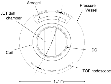
FIG. 1.: Cross-sectional view of the BESS spectrometer in its 1997 configuration. Overlayed is one of the $\bar{p}$ events.

Fig.1 shows a schematic view of BESS. It was designed [11] and constructed [12] as a high-resolution spectrometer to perform searches for rare cosmic-rays, as well as various precision measurements. A uniform field of 1 Tesla is produced by a thin (4 g/cm²) superconducting coil [13], through which particles can pass without too many interactions. The magnetic-field region is filled with the tracking volume. This geometry results in an acceptance of 0.3 m²sr, which is an order of magnitude larger than those of previous cosmic-ray spectrometers. The tracking is performed by fitting up to 28 hit-points in the drift chambers, resulting in a magnetic-rigidity ($R$) resolution of 0.5 % at 1 GV/$c$. The upper and lower scintillator-hodoscopes provide two d$E$/d$x$ measurements and the time-of-flight (TOF) of particles. The d$E$/d$x$ in the drift chamber gas is obtained as a truncated mean of the integrated charges of the hit-pulses. For the ’97 flight, the hodoscopes were placed at the outer-most radii, and the timing resolution of each counter was improved to 50 psec rms, resulting in $\beta^{-1}$ resolution of 0.008, where $\beta$ is defined as particle velocity [14] divided by the speed of the light. Furthermore, a Cherenkov counter with a silica-aerogel ($n$ = 1.032) radiator was newly installed [15], in order to veto $e^{-}/\mu^{-}$ backgrounds which gave large Cherenkov light outputs corresponding to 14.7 mean photo-electrons when crossing the aerogel.

The 1997 BESS balloon flight was carried out on July 27, from Lynn Lake, Canada. The scientific data were taken for 57,032 sec of live time at altitudes ranging from 38 to 35 km (an average residual air of 5.3 g/cm²) and cut-off rigidity ranging from 0.3 to 0.5 GV/$c$. The first-level trigger was provided by a coincidence between the top and the bottom scintillators, with the threshold set at 1/3 of the pulse height from minimum ionizing particles. The second-level trigger, which utilized the hit-patterns of the hodoscopes and the inner drift chambers (IDC), first rejected unambiguous null- and multi-track events and made a rough rigidity-determination to select negatively-charged particles predominantly. In addition, one of every 60 first-level triggers was recorded, in order to build a sample of unbiased triggers.

The off-line analysis [10] selects events with a single track fully contained in the fiducial region of the tracking volume with acceptable track qualities. The three d$E$/d$x$ measurements are loosely required as function of $R$ to be compatible with proton or $\bar{p}$. The combined efficiency of these off-line selections is 83 – 88 % for $R$ from 0.5 to 4 GV/$c$. These simple and highly-efficient selections are sufficient for a very clean detection of $\bar{p}$’s in the low-velocity ($\beta<0.9$) region. At higher-velocities, the $e^{-}/\mu^{-}$ background starts to contaminate the $\bar{p}$ band, where we require the Cherenkov veto; i.e., 1) the particle trajectory to cross the fiducial volume of the aerogel, and 2) the Cherenkov output to be less than 0.09 of the mean output from $e^{-}$. This cut reduces the acceptance by 20 %, but rejects $e^{-}/\mu^{-}$ backgrounds by a factor of 6000, while keeping 93 % efficiency for protons and $\bar{p}$’s which cross the aerogel with rigidity below the threshold (3.8 GV/$c$). Fig.2 shows the $\beta^{-1}$ versus $R$ plot for the surviving events. We see a clean narrow band of 415 $\bar{p}$’s at the exact mirror position of the protons. The $\bar{p}$ sample is thus mass-identified and background-free, as the cleanness of the band demonstrates and various background studies show. In particular, backgrounds of albedo and of mis-measured positive-rigidity particles are totally excluded by the excellent $\beta^{-1}$ and $R^{-1}$ resolutions. To check against the “re-entrant albedo” background, we confirmed that the trajectories of all $\bar{p}$’s can be traced numerically through the Earth’s geomagnetic field back to the outside of the geomagnetic sphere.

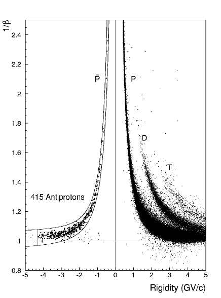
FIG. 2.: The identification of $\bar{p}$ events. The solid lines define the $\bar{p}$ mass band used for the spectrum measurement.

We obtain the $\bar{p}$ fluxes at the top of the atmosphere (TOA) in the following way: The geometrical acceptance of the spectrometer is calculated both analytically and by two independent Monte Carlo methods. The live data-taking time is directly measured by two independent scaler systems gated by the “ready” gate which controls the first-level trigger. The efficiencies of the second-level trigger and of the off-line selections are determined by using the unbiased trigger sample. The TOA energy of each event is calculated by tracing back the particle through the detector material and the air. The interaction loss of the $\bar{p}$’s is evaluated by applying the same selections to the Monte Carlo events generated by geant/gheisha, which incorporates [16] detailed material distribution and correct $\bar{p}$-nuclei cross sections. We subtract the expected number [17] of atmospheric $\bar{p}$’s, produced by the collisions of cosmic-rays in the air. The subtraction amounts to $9\pm 2$ %, $15\pm 3$ % and $19\pm 5$ %, respectively, at 0.25, 0.7 and 2 GeV, where the errors correspond to the maximum difference among three recent calculations [17, 18, 19] which agree to each other. Proton fluxes are obtained in a similar way. Atmospheric protons are subtracted by following Papini [20].

Table I contains the resultant BESS ’97 $\bar{p}$ fluxes and $\bar{p}/p$ flux ratios at TOA. The first and the second errors represent the statistical [21] and systematic errors, respectively. We checked that the central values of the fluxes are stable against various trial changes of the selection criteria, including uniform application of the Cherenkov veto also to the low $\beta$ region. The dominant systematic errors at high and low energies, respectively, are uncertainties in the atmospheric $\bar{p}$ calculations and in the $\bar{p}$ interaction losses to which we attribute $\pm$15 % relative error. As shown in Table I, the BESS ’97 fluxes are consistent [22] with the ’95 fluxes in the overlapping low-energy range (0.2 to 1.4 GeV). The solar activities at the time of the two flights were both close to the minimum as shown by world neutron monitors and by the low-energy proton spectra [23] measured by BESS.

TABLE I.: Antiproton fluxes (in $\times 10^{-2}$ m^-2s^-1sr^-1GeV^-1) and $\bar{p}/p$ ratios (in $\times 10^{-5}$) at TOA. T (in GeV) define the kinetic energy bins. ${\rm{N}}_{\bar{p}}$ and $\overline{\rm{T}}_{\bar{p}}$, respectively, are the number of observed antiprotons and their mean kinetic energy in each bin. The eighth bin of BESS ’95 flux actually covers the energy region from 1.28 to 1.40 GeV.

	BESS	’97			BESS	’95		BESS	’97+’95
T (GeV)	${\rm{N}}_{\bar{p}}$	$\overline{\rm{T}}_{\bar{p}}$	$\bar{p}$ flux	$\bar{p}/p$ ratio	${\rm{N}}_{\bar{p}}$	$\overline{\rm{T}}_{\bar{p}}$	$\bar{p}$ flux	$\overline{\rm{T}}_{\bar{p}}$	$\bar{p}$ flux	$\bar{p}/p$ ratio
0.18 - 0.28	4	0.21	$0.74^{+0.58\,+0.12}_{-0.34\,-0.12}$	$0.44^{+0.34\,+0.08}_{-0.20\,-0.08}$	3	0.24	$1.75^{+1.41\,+0.37}_{-1.13\,-0.37}$	0.22	$1.00^{+0.51\,+0.18}_{-0.42\,-0.18}$	$0.51^{+0.31\,+0.08}_{-0.19\,-0.08}$
0.28 - 0.40	9	0.35	$1.05^{+0.51\,+0.12}_{-0.36\,-0.12}$	$0.52^{+0.25\,+0.08}_{-0.18\,-0.08}$	3	0.34	$1.00^{+0.86\,+0.14}_{-0.66\,-0.14}$	0.35	$1.04^{+0.43\,+0.12}_{-0.31\,-0.12}$	$0.52^{+0.22\,+0.06}_{-0.16\,-0.06}$
0.40 - 0.56	16	0.49	$1.23^{+0.45\,+0.13}_{-0.34\,-0.13}$	$0.67^{+0.24\,+0.10}_{-0.18\,-0.10}$	6	0.49	$1.40^{+0.87\,+0.17}_{-0.58\,-0.17}$	0.49	$1.27^{+0.37\,+0.14}_{-0.32\,-0.14}$	$0.70^{+0.22\,+0.08}_{-0.16\,-0.08}$
0.56 - 0.78	31	0.66	$1.63^{+0.41\,+0.16}_{-0.37\,-0.16}$	$1.01^{+0.26\,+0.14}_{-0.23\,-0.14}$	8	0.67	$1.29^{+0.66\,+0.14}_{-0.54\,-0.14}$	0.66	$1.54^{+0.33\,+0.16}_{-0.30\,-0.16}$	$0.97^{+0.22\,+0.10}_{-0.19\,-0.10}$
0.78 - 0.92	19	0.85	$1.41^{+0.48\,+0.14}_{-0.42\,-0.14}$	$1.11^{+0.38\,+0.16}_{-0.33\,-0.16}$	6	0.83	$1.57^{+1.07\,+0.17}_{-0.71\,-0.17}$	0.85	$1.44^{+0.44\,+0.15}_{-0.36\,-0.15}$	$1.15^{+0.35\,+0.12}_{-0.29\,-0.12}$
0.92 - 1.08	16	1.01	$0.83^{+0.42\,+0.10}_{-0.32\,-0.10}$	$0.78^{+0.39\,+0.12}_{-0.30\,-0.12}$	5	0.99	$1.05^{+0.84\,+0.12}_{-0.65\,-0.12}$	1.01	$0.87^{+0.36\,+0.10}_{-0.32\,-0.10}$	$0.82^{+0.35\,+0.09}_{-0.27\,-0.09}$
1.08 - 1.28	32	1.19	$1.68^{+0.46\,+0.15}_{-0.41\,-0.15}$	$1.86^{+0.50\,+0.25}_{-0.46\,-0.25}$	7	1.18	$1.60^{+0.99\,+0.16}_{-0.82\,-0.16}$	1.19	$1.65^{+0.40\,+0.15}_{-0.36\,-0.15}$	$1.85^{+0.46\,+0.18}_{-0.41\,-0.18}$
1.28 - 1.52	43	1.40	$2.18^{+0.49\,+0.19}_{-0.44\,-0.19}$	$2.89^{+0.65\,+0.38}_{-0.59\,-0.38}$	5	1.33	$1.87^{+1.35\,+0.18}_{-1.08\,-0.18}$	1.39	$2.13^{+0.43\,+0.19}_{-0.39\,-0.19}$	$2.82^{+0.61\,+0.25}_{-0.54\,-0.25}$
1.52 - 1.80	51	1.65	$2.45^{+0.48\,+0.24}_{-0.44\,-0.24}$	$4.22^{+0.83\,+0.59}_{-0.76\,-0.59}$	-	-	-	1.65	$2.45^{+0.48\,+0.24}_{-0.44\,-0.24}$	$4.22^{+0.83\,+0.59}_{-0.76\,-0.59}$
1.80 - 2.12	51	1.96	$2.27^{+0.45\,+0.24}_{-0.42\,-0.24}$	$4.90^{+0.98\,+0.71}_{-0.90\,-0.71}$	-	-	-	1.96	$2.27^{+0.45\,+0.24}_{-0.42\,-0.24}$	$4.90^{+0.98\,+0.71}_{-0.90\,-0.71}$
2.12 - 2.52	64	2.31	$2.40^{+0.42\,+0.21}_{-0.37\,-0.21}$	$6.74^{+1.19\,+0.89}_{-1.03\,-0.89}$	-	-	-	2.31	$2.40^{+0.42\,+0.21}_{-0.37\,-0.21}$	$6.74^{+1.19\,+0.89}_{-1.03\,-0.89}$
2.52 - 3.00	56	2.72	$2.02^{+0.40\,+0.18}_{-0.35\,-0.18}$	$7.80^{+1.54\,+1.05}_{-1.34\,-1.05}$	-	-	-	2.72	$2.02^{+0.40\,+0.18}_{-0.35\,-0.18}$	$7.80^{+1.54\,+1.05}_{-1.34\,-1.05}$
3.00 - 3.56	23	3.25	$1.65^{+0.56\,+0.20}_{-0.44\,-0.20}$	$7.63^{+2.59\,+1.19}_{-2.04\,-1.19}$	-	-	-	3.25	$1.65^{+0.56\,+0.20}_{-0.44\,-0.20}$	$7.63^{+2.59\,+1.19}_{-2.04\,-1.19}$

FIG. 3.: BESS ’95+’97 (solar minimum) antiproton fluxes at the top of the atmosphere together with previous data. The error-bars represent the quadratic sums of the statistical and systematic errors. The curves are recent calculations of the secondary $\bar{p}$ spectra for the solar minimum period.

Shown in Fig.3 is the combined BESS (’95+’97) spectrum, in which we detect for the first time a distinctive peak at 2 GeV of secondary $\bar{p}$, which clearly is the dominant component of the cosmic-ray $\bar{p}$’s.

The measured secondary $\bar{p}$ spectrum provides crucial tests of models of propagation and solar modulation, since one has a priori knowledge of the input source spectrum for the secondary $\bar{p}$, which can be calculated by combining the measured proton and helium spectra with the accelerator data[24] on the $\bar{p}$ production. The distinct peak structure of the $\bar{p}$ spectrum also has clear advantages in these tests over the monotonic (and unknown) source spectra of other cosmic-rays.

The curves shown in Fig.3 are recent theoretical calculations for the secondary $\bar{p}$ in diffusion model [25, 26] and leaky box model [27, 28], in which the propagation parameters (diffusion-coefficient or escape length) are deduced by fitting various data on cosmic-ray nuclei such as Boron/Carbon ratio, under the assumption that the different cosmic-ray species (nuclei, proton and $\bar{p}$) undergo a universal propagation process. These calculations                                                                           use as essential inputs recently measured proton spectra [23, 31, 32], which are significantly (by a factor 1.4 to 1.6) lower than previous data in the energy range (10 to 50 GeV) relevant to the $\bar{p}$ production.

FIG. 4.: BESS ’95+’97 $\bar{p}/p$ flux ratios with previous data [9] and the theoretical calculations.

These calculations reproduce our spectrum at the peak region remarkably well within their $\pm$15 % estimated accuracy [28]. This implies that the propagation models [33] are basically correct and that different cosmic-ray species undergo a universal propagation process.

At low energies, the calculations predict somewhat diverse spectra reflecting various uncertainties [34], which presently make it difficult to draw any conclusion on possible admixture of primary $\bar{p}$ component. As noted in Ref.[5], the rapid increase of solar activity toward the year 2001 will drastically suppress the primary $\bar{p}$ component such as from the primordial black holes [3], while changing the shape of the secondary $\bar{p}$ only modestly [27]. This will help us to separate out the “primary” and “secondary” components at low energies. Future annual BESS flights will thus be important to search for primary $\bar{p}$ component, to study solar modulation, and to investigate further details of the propagation.

Since most previous data were presented in the form of $\bar{p}/p$ flux ratios [9], a compilation is made in Fig.4, which shows again the unprecedented accuracy of our measurement.

Sincere thanks are given to NASA and NSBF for the balloon launch. The analysis was performed by using the computing facilities at ICEPP, Univ. of Tokyo. This experiment was supported by Grant-in-Aid from Monbusho in Japan and by NASA in the USA.

REFERENCES

- [1] R. L. Golden et al., Phys. Rev. Lett. 43, 1196 (1979).
- [2] T. K. Gaisser and R. K. Schaefer, Astrophys. J. 394, 174 (1992).
- [3] S. W. Hawking, Commun. Math. Phys. 43, 199 (1975).
- [4] K. Maki et al., Phys. Rev. Lett. 76, 3474 (1996).
- [5] T. Mitsui et al., Phys. Lett. B 389, 169 (1996).
- [6] E. A. Bogomolov et al., Proc. 16th Int. Cosmic Ray Conf. (Kyoto) 1, 330 (1979).
- [7] K. Yoshimura et al., Phys. Rev. Lett. 75, 3792 (1995); A. Moiseev et al., Astrophys. J. 474, 479 (1997).
- [8] J. W. Mitchell et al., Phys. Rev. Lett. 76, 3057 (1996).
- [9] M. Boezio et al., Astrophys. J. 487, 415 (1997), and references therein.
- [10] H. Matsunaga et al., Phys. Rev. Lett. 81, 4052 (1998).
- [11] S. Orito, in Proceedings of the ASTROMAG Workshop (KEK Report 87-19, 1987), p.111.
- [12] Y. Ajima et al., submitted to Nucl. Instrum. Methods.
- [13] A. Yamamoto et al., IEEE Trans. Magn. 24, 1421 (1988).
- [14] is defined to be positive for down-going particles.
- [15] Y. Asaoka et al., Nucl. Instrum. Methods A 416, 236 (1998)
- [16] H. Matsunaga, Ph.D. thesis, University of Tokyo, 1997.
- [17] T. Mitsui, Ph.D. thesis, University of Tokyo, 1996.
- [18] Ch. Pfeifer et al., Phys. Rev. C 54, 882 (1996).
- [19] S. A. Stephens, Astropart. Phys. 6, 229 (1996).
- [20] P. Papini et al., Nuovo Cimento 19C, 367 (1996).
- [21] G. J. Feldman et al., Phys. Rev. D 57, 3873 (1998).
- [22] Our ’97 data have a factor 2.7 times more statistics than ’95 data in the overlapping low-energy region. This is realized by combination of longer flight-time, less dead-time and higher trigger- and selection-efficiencies.
- [23] T. Sanuki et al., in New Era in Neutrino Physics, Universal Academy Press, 1998, and to be published.
- [24] L. C. Tan and L. K. Ng, J. Phys. G 9, 227 (1983).
- [25] A. Bottino et al., Phys. Rev. D 58, 123503 (1998).
- [26] L. Bergström et al., astro-ph/9902012.
- [27] J. W. Bieber et al., astro-ph/9903163.
- [28] T. Mitsui et al. (to be published): The spectra were calculated in the leaky box model. For the tertiary interaction of , a phenomenological model which fits data well was used instead of flat energy distribution of the emerging usually assumed. Examples of the escape length () were used, including a dependent obtained in Ref.[29], and a dependent only on . The spectra were solar-modulated by following Fisk [30].
- [29] S. A. Stephens et al., Astrophys. J. 505, 266 (1998).
- [30] L. A. Fisk et al., J. Geophys. Res. 76, 221 (1971).
- [31] W. Menn et al., Proc. 25th Int. Cosmic Ray Conf. (Durban) 3, 409 (1997).
- [32] M. Boezio et al., Astrophys. J. 518, 457 (1999).
- [33] The diffusion and leaky box models are expected to be equivalent for stable cosmic-rays which are produced and interact only in the thin disk, as should be the case for secondary . See V. S. Berezinskii et al., Astrophysics of cosmic rays (North-Holland, Amsterdam, 1990).
- [34] The main differences among the calculations are the treatment of the tertiary interactions, nuclear models to simulate proton-nucleus and nucleus-proton interactions, the and dependences of the propagation parameter, and the solar modulations.