The roughness of the last scattering surface

Abstract

We propose an alternative analysis of the microwave background temperature anisotropy maps that is based on the study of the roughness of natural surfaces. We apply it to large angle anisotropies, such as those measured by COBE–DMR. We show that for a large signal to noise experiment, the spectral index can be determined independently of the normalization. We then analyze the 4 yr COBE map and find for a flat $\Omega=1$ universe, that the best-fitting value for the spectral index is $n=1.15^{+0.39}_{-0.34}$ and for the amplitude $Q_{rms-PS}=14.1^{+3.9}_{-3.5}\mu K$. For $n=1$, the best-fitting normalization is $Q_{rms-PS}|_{n=1}=16.2^{+1.4}_{-1.3}\mu K$.

1 Introduction

The measurement of the cosmic microwave background temperature anisotropies at large angular scales by the COBE satellite has provided a unique insight to the universe inhomogeneities at the recombination time. It is believed that these anisotropies originated from small perturbations in the gravitational potential and thus they give information about the inhomogeneities at the linear evolution stage, avoiding most of the complications associated to the study of the non-linear evolution of structures.

Since the discovery of the anisotropies, several statistical analysis of the data were proposed. The most widely used ones are the two point correlation function (Hinshaw et al. 1996a ) and the angular power spectrum (Wright et al. (1996); Górski et al. (1996); Hinshaw et al. 1996b ; Tegmark (1996, 1996); Bautista & Torres (1996); Bunn & White (1997); Bond et al. (1997)). These statistics contain a complete description of the anisotropies if they are Gaussian distributed, and thus are the most natural choice to test cosmological models leading to Gaussian primordial fluctuations. However, there are also possible physical mechanisms which produce non–Gaussian distributed anisotropies. Motivated by this possibility, other statistical analysis of the anisotropy maps, which are not shaped for Gaussian fields, have been developed. These include the study of higher order correlation functions (Hinshaw et al. (1995)) and morphological characteristics of hot and cold spots, as genus and density of spots (Torres et al. (1995); Kogut (1996); Fabbri & Torres (1996)), Minkowski functionals (Schmalzing & Górski (1998)) and multifractal studies (Pompilio et al. (1995); Diego et al. (1999)). It is quite remarkable that Gouveia Dal Pino et al. (1995) find a fractal behavior for the COBE–DMR first year data using the perimeter–area relation of iso–temperature contour regions. Whereas the topological analyses give information about the invariant quantities under deformations, the multifractal analyses shed light on the self-similarity of the field. Although the first analysis of the COBE maps, based on the three-point correlation function indicated that the anisotropies are consistent with Gaussianity (Kogut (1996)), the recent analysis of the bispectrum by Ferreira et al. (1998) argues for evidence of non–Gaussianity in the COBE maps. Whether this effect can be explained by some still unrecognized foreground contamination or is a real signal of CMB non–Gaussianity is still an open question.

Both sets of statistical analysis, those based on the angular spectrum and the topological ones, have been extensively applied to the COBE–DMR anisotropy maps and several determinations of the amplitude of the inhomogeneities (usually parameterized in terms of the resulting quadrupole amplitude $Q_{rms-PS}$, that we abbreviate as $Q$) and of the primordial spectral index $n$ have been obtained. These determinations had an extraordinary impact on cosmological models as they provide the first accurate measure of the amplitude of the primordial fluctuations (see Bennett et al. (1996); Banday et al. (1997) for a summary of the 4 yr COBE analysis and the references above for the other analyses). Most of these determinations show a strong anticorrelation between the inferred values for $Q$ and $n$.

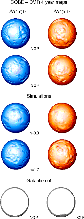
Figure 1: The four top spheres represent the anisotropies of the 4–year COBE–DMR maps. The two upper ones are centered in the North Galactic Pole (NGP), while the other two are in the South Galactic Pole (SGP). On the left–hand side, in blue, pixels where $\Delta T<0$ are depicted as depths, while on the right–hand side, in red, pixels where $\Delta T>0$, are displayed as heights. The ‘sea–level’ in each blue (red) sphere corresponds to the pixels where $\Delta T\geq 0$ ($\Delta T\leq 0$). Below, spheres centered only at the NGP are similarly displayed and correspond to two simulations with spectral indices $n=0.3$ and $n=1.7$. A smoothing filter of $7^{\circ}$ (full width at half maximum) has been applied to the COBE data to reduce the effect of the radiometer noise. In all cases the height of the pixels lying within the customized Galactic cut has been fixed to zero, and therefore those pixels belong to the ‘sea–level’. The segments of the maps corresponding to the Galactic cut are displayed in grey at the bottom panels.

We propose here an alternative approach to the analysis of the anisotropies, which is inspired in the study of the roughness of natural surfaces in fields like geology, biology or metallurgy. Many of the natural surfaces can be modeled as fractals and a central concept related to their roughness is that of the fractal dimension. The dimension index for fractal surfaces lies between 2 and 3 and it depends on the irregularity of the surface. By associating to every point in a sphere a height (or depth) proportional to the excess (or defect) of the temperature measured in that direction with respect to the mean, we obtain an irregular surface which roughness is directly related to the temperature anisotropies. In Figure 1 we show the COBE–DMR 4 yr map of the CMB anisotropies by means of this procedure. The blue (red) spheres represent the pixels where $\Delta T<0$ ($\Delta T>0$) as depths (heights) over a ‘sea–level’. In each pair of complementary spheres the ‘sea–level’ represents the pixels where $\Delta T\geq 0$ for the blue ones and $\Delta T\leq 0$ for the red ones. In this paper, we study how to obtain information about the primordial inhomogeneities from the analysis of the roughness of these surfaces using fractal techniques.

The outline of the paper is as follows. In section 2 we briefly describe the most appropriate approach to measure the surface fractal dimension, we present an analytical relation between the spectral index and the fractal dimension and discuss the limitations of the procedure of trying to measure the fractal dimension and to determine the spectral index for actual sky data. In section 3 we apply these techniques to simulations of the COBE–DMR maps, and present a method to determine the spectral index, when the radiometer noise can be neglected. In Section 4 we present a modified method which can be used in small signal to noise maps to obtain a joint determination of $Q$ and $n$, we test it with simulations of the COBE–DMR maps, and we apply it to 4 yr map. Section 5 contains the conclusions.

2 Determination of the fractal dimension of a surface

Simple objects like points, segments, disks or spheres have dimensions 0, 1, 2 and 3 respectively. In between them there exist more complex objects with non-integer dimension. Irregular surfaces have fractal dimension between 2 and 3 depending on how much volume they fill. The fractal dimension is thus a useful tool to describe the roughness of surfaces (Mandelbrot (1982)). Different methods have been proposed in the literature to estimate it. One possibility could be to section the surface with a plane, measure the dimension of the profile and use the fact that the fractal dimension of the surface is one plus the dimension of the profile. The other possibility is to use algorithms that directly estimate the dimension of the surface. Some of the algorithms to evaluate the fractal dimension of profiles and surfaces have been comparatively tested by Dubuc et al. 1989a and Dubuc et al. 1989b , who also proposed an improved algorithm, the variation method. This is specially well suited when dealing with profiles or surfaces defined by a function of one or two variables respectively. In these cases one of the coordinates describing the profile or surface is of a different nature than the other(s). For example, the surface that we want to analyze can be described by two angular coordinates and a third one measuring temperature differences. One would like that the associated dimension be independent of the choice of the units in which the function is measured. The variation algorithm assigns the same fractal dimension to the surfaces defined by a function $f$ and by the function $Cf$, with $C$ a constant (it is invariant under affine transformations). The various methods to estimate the fractal dimension are obtained from the discretization of different definitions. Although they are mathematically equivalent in the continuum limit (Falconer (1990)), they can give different results when adapted to discrete sampled data. This is the case for the Minkowski–Bouligand (MB) dimension and the box dimension. They can both be defined as

$$D=\lim_{L\to 0}\left(3-\frac{\log V(L)}{\log L}\right),$$ (1)

where $V(L)$ is the volume of a covering of the surface, which in the case of the MB dimension is the set of all points at a distance less than $L$ from a point of the surface (or the union of all the balls of radius $L$ centered on a point of the surface). In the box dimension case, $V(L)$ is the volume of the union of disjoint cubes of side $L$ needed to cover the surface. Algorithms implementing these definitions calculate $V(L)$ for some values of $L$ and then recover $D$ from the slope of the $\log V$–$\log L$ plot. Both methods have the problem pointed out before, they give different results when applied to functions $f$ and $Cf$. The variation method (Dubuc et al. 1989b ) overcomes this difficulty by defining a new covering of the surface in the following way. If the surface is described as a set of points $(x,y,f(x,y))$, it associates to each point of the surface an upper point as the maximum of the function in an $L$–neighborhood $[x-L,x+L]\times[y-L,y+L]$ and a lower point as the minimum of the function in that neighborhood. $V(L)$ is the volume of the region between the upper and lower surfaces (or the volume of the union of all the squares $[x-L,x+L]\times[y-L,y+L]$ centered on a point of the surface and truncated to the region $(x,y)$ covered by the surface). Once again, $D$ is obtained from the slope of the $\log V$–$\log L$ plot. Theoretically, we would expect a constant slope for a fractal surface. However, the constant slope is only obtained in practice for an intermediate range of scales, which are large enough so that there is a statistically good sampling of every point neighborhood, and small enough compared to the total sample size. As we will see, these conditions are problematic for the application to large angle anisotropy maps, as the DMR ones. Nevertheless, the method can be adapted to extract useful information from the data.

To illustrate the connexion between fractals and the CMB, let us suppose that the Sachs Wolfe effect gives the main contribution to the anisotropies. In this case, large angle CMB anisotropies can be described as a fractal, with dimension related to the spectral index of the gravitational potential from which they originated. They resemble in fact one of the most frequently used mathematical models to construct random fractals, the fractional Brownian functions (FBF) (Mandelbrot & van Ness (1986)). For one variable, the fractional Brownian motion is a single–valued function, which increments, $F(t_{2})-F(t_{1})$, have a Gaussian distribution with variance $\langle|F(t_{2})-F(t_{1})|^{2}\rangle\propto|t_{2}-t_{1}|^{2H}$, where the brackets denote the ensemble average over many samples, and the parameter $H$ has a value $0<H<1$. The value $H=1/2$ corresponds to the well–known Brownian motion. The FBF show a statistical scaling behavior: for a function of $E$ Euclidean dimensions, if ${\bf x}=(x_{1},...,x_{E})$ is scaled by a factor $r$, $\Delta F$ is changed by a factor $r^{H}$, namely $\langle|\Delta F(r{\bf x})|^{2}\rangle=r^{2H}\langle|\Delta F({\bf x})|^{2}\rangle$. This scaling by a different factor for ${\bf x}$ and $F({\bf x})$ is known as self–affinity. It can be seen that the fractal dimension associated to this kind of function is $D=E+1-H$ (Voss (1988)). The power spectrum of a FBF is a power law and the spectral index is directly related to the parameter $H$, and thus to $D$. In fact, a widely used algorithm to construct a FBF with a given fractal dimension $D$ is to obtain a random function with the required power–law spectrum by a Fourier transformation (Saupe (1988)). According to this, the CMB anisotropies originated through the Sachs–Wolfe effect by a gravitational potential $\Phi({\bf x},t)$ with power spectrum $P(k)=Ak^{n-4}$ in a flat $\Omega=1$ universe can be described by a FBF. We can directly obtain the parameter $H$ from the computation of

$$\langle|\Phi({\bf x}+{\bf y})-\Phi({\bf x})|^{2}\rangle=\frac{A}{\pi^{2}}\int_{0}^{\infty}dk\ k^{n-2}\left(1-\frac{\sin(ky)}{ky}\right)\propto y^{1-n}$$ (2)

where $y$ is the physical distance between the two points. If we consider points on a sphere, it is given by $y=2r\sin(\theta/2)$, with $r$ the radius of the sphere and $\theta$ the angular separation between the points. This relation holds for $-1<n<1$, that is the range in which the integral in eq. (2) converges. Thus, $H$ is directly related to the spectral index $n$ by the equality $2H=1-n$. We can hence in principle determine the spectral index $n$ by measuring the fractal dimension of the surface constructed by assigning to every point on a sphere a height (or depth) proportional to the temperature excess (or defect) in that direction. These are related by $D=3-H=(5+n)/2$. Spectral indices larger than $n=1$ saturate in the fractal dimension $D=3$ as a surface cannot have a larger fractal dimension. We would like to stress that the fractal dimension is independent of the spectrum normalization, it only depends on the spectral index. This is due to the fact that $D$ does not change when the function is multiplied by a constant factor because of the self–affinity property already discussed. Let us note that this discussion applies to the simplest case of a flat universe, with vanishing cosmological constant and constant spectral index at the large angular scales tested by COBE, where the Sachs–Wolfe effect gives the dominant contribution to the anisotropies. In the case of a non-vanishing cosmological constant or an open universe there are additional contributions to the anisotropies due to the time variation of the gravitational potential along the photons path. At smaller angular scales the acoustic oscillations of the photon-baryon plasma at recombination give the dominant contribution to the anisotropies and thus no scaling is expected.

In practice, however, it is not possible to determine $n$ through the above mentioned analytical relation with $D$. There are some difficulties to use it in actual maps of the sky measuring large angular scale anisotropies as the DMR ones. The main problem comes from the fact that the size of the surface is limited by the solid angle of the sphere (in fact, even smaller due to the Galactic cut). This constrains the maximum number of points at which the surface is sampled. The COBE–DMR maps give the temperature at 6144 pixels, that reduce to approximately 4000 when the Galactic cut is taken into account. In order to be able to determine the fractal dimension $D$ of a surface from the slope of the log$V$–log $L$ plot, we need to have a large enough sampling of the surface so that we pick a range of $L$ values in which the plot has a constant slope (we have already pointed out that deviations of this behavior are expected both at large scales, close to the size of the sample, and small scales, close to the spacing of the sampling points). We have found using synthetic fractals that in order to see the constant slope region in the plot we need a sampling of at least $10^{6}$ points. We constructed two-dimensional FBF with various values of the fractal dimension and for various sizes of the sample. Only when the number of sampling points was larger than $(1024)^{2}$ a plateau in the $D(L)$ plot was evident. This means that we would need to have a much larger number of pixels than in the COBE maps. If we have to work with a smaller number of pixels, the slope of the plot will not show a plateau and we cannot obtain $D$ directly from its value (and $n$ from the analytical relation). Nevertheless, even if the slope varies with the scale, surfaces constructed with different $n$ show a different behavior of the slope vs. scale relation, $D(L)$, and this can be used to identify the underlying spectral index, as is shown in the next section. Another point to be taken into account is that the maps have the dipole subtracted. The dipole is mostly due to the proper motion of the Earth, and as this contribution cannot be separated from a primordial one, it is completely subtracted from the maps. This procedure breaks the scaling present in eq. (2) and hence also interferes in the determination of $D$. The last point that we have to consider is the effect of the instrumental noise, but we will leave its discussion until section 4. Let us first consider the determination of $n$ in a very high signal to noise experiment.

3 Ideal noiseless experiment

We can see that the slope of the $\log V$–$\log L$ plot has a strong enough dependence on the spectral index to be a useful tool to determine $n$ by testing the predictions of a large number of Monte Carlo simulations of the maps for a range of $n$ values (we assume a flat $\Omega=1$ universe). For definiteness, we consider the COBE–DMR experiment with all its actual characteristics, as pixelization and beam smearing (Bennett et al. (1996)), but we neglect for the moment the radiometer noise. We use a $|b|<20^{\circ}$ Galactic cut. Thus, considering the quadrilaterized spherical cube pixelization used by the COBE team and cutting the Galaxy, our surface consists of two pieces corresponding to the two uncut faces of the cube, including the north and south Galactic poles respectively, with adjacent strips coming from the cut faces. Each complete face has $32^{2}$ pixels, while the strips have approximately 8 pixels width. For each of these pixels, we have a value of $\Delta T/T$ as it would be measured by an observer with an ideal radiometer.

We have adapted the variation method (Dubuc et al. 1989b ) to this surface in order to determine the $V(L)$ curve. In this algorithm, the volume associated to a scale $L$ is given by the region located between a top and a bottom surface constructed in the following way. To each pixel we associate an upper (lower) point at scale $L$ by the maximum (minimum) of the $\Delta T/T$ corresponding to the pixels in a square of side $L$, centered on that pixel. These points form the top (bottom) surface. We only consider scales corresponding to an integer number of pixels. Points located near the borders, i.e. close to the Galactic cut are problematic. Standard border corrections (as multiplying by the fraction of the area corresponding to the missing region) are not useful to look for maxima and minima, thus we deal with the problem in another way. First, we consider the surface formed by the two complete faces, the north and the south ones, and use the pixels in the strips coming from the cut faces only for the computation of the maxima and minima to be associated to the points close to the borders in the north and south faces. This is a compromise solution between loosing some information from the cut face pixels and reducing the need for border corrections. At the largest scales, where problems with edge effects remain for some pixels, we changed the region to another one, with approximately the same area in the pixel neighborhood. We followed the implementation of the algorithm proposed by Dubuc et al. 1989b . After obtaining the volume associated to the surface at scales $L$ from 2 to 30 pixels (in steps of 2), we computed the local dimension as the slope of a five-point log-log linear regression of $V/L^{3}$ vs. $1/L$. This local dimension is regarded as a ‘sliding window’ estimate (through the scale) of the fractal dimension (Dubuc et al. 1989a ). As discussed above, a constant slope $D$ characterizes a fractal surface of fractal dimension $D$.

We also perform a second kind of analysis to the maps, that makes full use of the cut faces data and does not suffer from border effects. This consists in making a one–dimensional study of the $\Delta T/T$ profiles along lines parallel to the Galactic cut. As these are closed lines, there are no borders. There are seven of these complete lines of pixels to the north and other seven to the south of the Galactic cut, each one is 128 pixels long. The analysis of these profiles is similar to that performed on the surface, but now we compute the area of the surface covering the profile. For each of the 14 profiles that we analyze in a map, we obtain the area $S$ of the covering surface at scales $L$ from 3 to 41 (in steps of 4) and we take a mean over them. We then compute the slope of the $\log(S/L^{2})$ vs. $\log(1/L)$ plot by fitting a line to each group of five consecutive points. A fractal profile with dimension $D$ (between 1 and 2) would have a constant slope equal to $D$.

We have performed the surface and profile analysis on Monte Carlo simulations of the COBE–DMR maps for different values of the spectral index $n$. We used 500 simulations of the maps for each value of $n$ from 0.3 to 1.7 (in steps of 0.1). Even if we neglect the radiometer noise, we do not expect a unique result for different realizations with the same spectral index due to the cosmic variance. The distribution of the results for the 500 simulation with a given $n$ is a measure of the results that observers located at different positions would obtain. The mean curves of the slopes as a function of the scales over the 500 simulations for the surface analysis, $D_{S}(L)$, and for the profile analysis, $D_{P}(L)$, show a clear ordering according to their spectral index, as can be seen in Figure 2. In both cases, the larger $n$ have larger slopes associated at all scales. This result reflects the fact that a larger spectral index gives rise to a rougher surface as it is clearly illustrated by the comparison of the spheres corresponding to $n=0.3$ and $n=1.7$ in Figure 1 (Plate 1)

This property can be used to infer the most probable value of $n$ associated to a (noiseless) map. For each of the simulated maps, we construct a six–dimensional vector $d_{i}$, with the first three components given by the $D_{S}(L)$ values at three different scales and the last three components by the $D_{P}(L)$ values at three different scales. In this way, combining the information from the surface and profile analysis, we make full use of the signal in the cut and uncut faces. The choice of the three scales for each set is enough, as each point contains information from five consecutive points in the $V(L)$ or $S(L)$ curves. The inclusion of more points does not diminish the resulting dispersions. The $\chi^{2}$ statistics is then obtained as

$$\chi^{2}=\sum_{i=1}^{6}\sum_{j=1}^{6}\left(\langle d_{i}\rangle-d_{i}^{M}\right)M_{ij}^{-1}\left(\langle d_{j}\rangle-d_{j}^{M}\right),$$ (3)

where $\langle d_{i}\rangle$ is the mean of the $d_{i}$ computed from the 500 simulations of the maps for a given $n$ and the covariance matrix is given by

$$M_{ij}=\frac{1}{N}\sum_{k=1}^{N}\left(d_{i}^{k}-\langle d_{i}\rangle\right)\left(d_{j}^{k}-\langle d_{j}\rangle\right),$$ (4)

with $N=500$, the number of realizations used. We denoted by $d_{i}^{M}$ the slopes obtained for the map that we want to analyze. The likelihood statistics ${\cal L}$ is given by

$${\cal L}=\frac{1}{(2\pi)^{m/2}(\det M)^{1/2}}\exp(-\chi^{2}/2),$$ (5)

with $m=6$, the number of data points used in the fit.

We tested the method by using as input data 100 simulations with $n=1$. We first computed the $d_{i}^{M}$ for each of them and then obtained $\chi^{2}$ for the different $n$ values. We fitted a parabola and associated the value of $n$ at the minimum as the best-fitting $n$ to the data. The returned values of $n$ for the 100 simulations have mean $\langle n\rangle=1.01$ and dispersion $\sigma_{n}=0.16$. A similar analysis using the maxima of the likelihood returned $\langle n\rangle=1.02$ and $\sigma_{n}=0.19$. Thus, both methods work reasonably well to determine $n$, the dispersion measures the cosmic variance. As noted before, this determination is independent of the amplitude of the spectrum (or the value of $Q$).

When analyzing actual sky maps, we have to take into account the radiometer noise. For maps with a high signal to noise ratio we expect that an analysis following the line presented in this section will lead to a rather good determination of $n$. However, when dealing with low signal to noise maps, like the DMR one, this method is not useful anymore. By one side, the ordering of the curves $D_{S(P)}(L)$ with respect to the $n$ value is not maintained at all scales, but they cross in the small scales region, where the noise is more important. Moreover, the method is no more independent of $Q$, the reason being that the amplitude of the noise introduces an intrinsic scale. Hence, a rescaling by a constant factor of the sky signal does not change the map by a constant factor, and the slope curves are no more independent of $Q$. We can however use a modified strategy to obtain the $Q$ and $n$ best-fitting values.

4 Analysis of the DMR data

In order to obtain the simultaneous determination of $Q$ and $n$ it is more useful to work directly with the volume of the coverings of the surface as a function of the scale, $V(L)$, instead of the slopes, $D_{S(P)}(L)$, as the former are more sensitive to the amplitude of the spectrum (or $Q$). In fact, in the noiseless case it was useful to work with the slopes because they provide a measure of the roughness that is independent of the amplitude. As we are now interested in determining also the amplitude, it is convenient to go a step back and work with the volume of the coverings.

We proceed in a way closely related to the analysis of the surface in the last section. In this case, in order to have a smoothly varying field and reduce the effect of the radiometer noise, we applied a Gaussian smoothing filter of $7^{\circ}$ (full width at half maximum) to the maps before starting the analysis. For every map that we analyze we obtain the volume of the covering of the surface at eight different scales ranging from 2 to 28 pixels. To deal with the border problems, we consider the surface formed by the two uncut faces, while we use the data in the cut faces to compute the minima and maxima as in the last section. The map used for our analysis is a weighted combination of the 53 and 90 GHz maps with the custom Galaxy cut (including the Orion and Ophiuco regions) of the 4 yr COBE–DMR data (Bennett et al. 1996), as released by the NSSDC. We simulate 500 maps following the characteristics of the map just mentioned, including the corresponding noise of the DMR combination for each individual pixel. We use for the multipole amplitudes the power-law expression by Bond & Efstathiou (1987); Fabbri et al. (1987), that is a very good approximation at large scales for a matter dominated universe (this can be readily generalized and can consider the case of a cosmological constant or curvature dominated universe using the multipoles obtained with the CMBFAST code (Seljak & Zaldarriaga (1996))). We consider values of $Q$ between 5 and 30 $\mu$K (in steps of 1 $\mu$K) and values of $n$ between $0$ and $2.2$ (in steps of 0.1). The curves $\log V(L)$ vs $\log L$ show an ordering, with larger $V$ associated to larger $Q$ for a fixed $n$, and to larger $n$ for a fixed $Q$. We used these curves to test which is the model that best fits the data. In figure 3 we compare the curves $\log V(L)$ for several models with the one for the data.

The $\chi^{2}$ statistics is in this case given by

$$\chi^{2}=\sum_{i=1}^{8}\sum_{j=1}^{8}\left(\langle\log V_{i}\rangle-\log V_{i}^{M}\right)M_{ij}^{-1}\left(\langle\log V_{j}\rangle-\log V_{j}^{M}\right),$$ (6)

where $\langle\rangle$ denotes the mean over the 500 simulations of the maps for a given $Q$ and $n$, and the covariance matrix is given by

$$M_{ij}=\frac{1}{N}\sum_{k=1}^{N}\left(\log V_{i}^{k}-\langle\log V_{i}\rangle\right)\left(\log V_{j}^{k}-\langle\log V_{j}\rangle\right).$$ (7)

The likelihood is defined as in eq. (5), with $m=8$. We consider here more scales than in the analysis of the slopes performed in Section 3 because there the local dimension, being the slope at a given scale, contains information from all scales within the considered sliding window. For a given map, we identify as the most probable values of $Q$ and $n$ those which maximize ${\cal L}$. The choice of eight points uses information from as many scales as possible without suffering numerical inaccuracies from inverting a matrix that becomes very degenerate since the information from different scales is strongly correlated.

We tested the accuracy of this method by applying it to simulations of the DMR maps as input. We used 900 simulations with $Q_{in}=18\mu K$ and $n_{in}=1$ and we obtained for each of them the values $Q_{ML}$ and $n_{ML}$ that maximize the likelihood. The returned values for $Q_{ML}$ have a mean $\langle Q_{ML}\rangle=18.4\mu K$ and a dispersion $\sigma_{Q}=4.4\mu K$, while the returned values for $n_{ML}$ have a mean $\langle n_{ML}\rangle=0.99$ and a dispersion $\sigma_{n}=0.33$. Thus, the bias is very small both for the spectral index as well as for the amplitude estimation.

The analysis of the 4 yr DMR data with this method returns as the best-fitting values $Q=14.1^{+3.9}_{-3.5}\mu K$ and $n=1.15^{+0.39}_{-0.34}$, where we have assigned the $68\%$ credible interval to $Q$ and $n$ by marginalizing the two–dimensional likelihood ${\cal L}(Q,n)$. The likelihood function shows a strong anticorrelation between our estimates of $Q$ and $n$. This can clearly be seen in Figure 4, which shows the contour plots corresponding to the $68\%$ and $95\%$ confidence regions of the likelihood function in the $Q-n$ plane. The contours show a significant elongation along a line that can be parameterized by $Q(n)=32.\times\exp(-0.69n)$. These results are consistent with a scale invariant power spectrum, in this case the best-fitting normalization is given by $Q_{rms-PS}|_{n=1}=16.2^{+1.4}_{-1.3}\mu K$. These estimates are in agreement with the results of the COBE group analysis of the data. Bennett et al. (1996) summarize their 4 yr results for the spectrum and normalization as $n=1.2\pm 0.3$ and $Q=15.3^{+3.8}_{-2.8}\mu$K, with the various analysis performed leading to very close values. The determinations of $n$ and $Q$ presented in this paper have both a central value slightly below the COBE ones, but well within the 1$\sigma$ range. For the scale invariant spectrum $n=1$, our normalization is 1$\sigma$ below the central value reported by the COBE group, $Q|_{n=1}=18.\pm 1.6\mu$K. The error bars are comparable. Results consistent with those presented in this paper are obtained by a multifractal analysis of the DMR data (Diego et al. (1999)).

We would like to note that in the previous analysis we have only considered the effect of scalar perturbations on the CMB anisotropies. However, in many models of inflation leading to $n<1$ spectra, primordial gravitational waves also give a relevant contribution to large scale anisotropies (see e.g. Lucchin et al. (1992)). This leads to a decrement of the value of $Q$ associated to a given map (Crittenden et al. (1993)). The gravitational wave contribution is negligible for most inflationary models leading to $n>1$ (Mollerach et al. (1994)), and thus the amplitude determination is not affected in this case.

5 Conclusions

We have proposed a new method to analyze temperature anisotropy maps that is based on the study of the roughness of a surface which has heights and depths proportional to the temperature sky anisotropies. For large angle anisotropies produced by the Sachs–Wolfe effect such surface should correspond to a fractal surface, with fractal dimension $D$ directly related to the spectral index $n$ of the primordial fluctuations. Thus, the determination of $D$ with known techniques developed for that purpose in other fields of science would lead to a determination of $n$. Unfortunately, we found that the range of angular scales over which the Sachs–Wolfe effect dominates is not large enough to allow a sampling of the surface in enough points for obtaining a direct determination of $D$ as the constant value of the plateau in the $D(L)$ plot. However, this does not preclude a determination of $n$ for large signal to noise anisotropy maps. We showed that in this case the whole (non-constant) $D(L)$ curve depends strongly on the spectral index and thus provide a useful tool to measure $n$. We tested this method with noiseless simulated maps and showed that it returns an accurate determination of the spectral index. All this procedure is independent of the overall normalization of the map.

For low signal to noise maps, the previous method is no longer useful to determine $n$ because the $D(L)$ curves for different $n$ cross at small scales where the noise is more relevant. Furthermore, the relative normalization of the signal to the amplitude of the noise also determines the shape of the $D(L)$ curve (it is no longer function of $n$ alone). To overcome this problem, we proposed an alternative method, in which the curve $V(L)$, corresponding to the volume of the surface covering vs. scale, is used instead of $D(L)$. This procedure allows a joint determination of $Q$ and $n$ in this case. The tests with simulated data showed that the estimated values are unbiased, and have reasonable error bars. The results of the application of this method to the COBE–DMR data, assuming a flat $\Omega=1$ cosmological model, are fully compatible with those of more standard analysis.

Let us note that although the original motivation was to determine the (constant) spectral index at large scales measuring the fractal dimension $D$, the methods developed in Sections 3 and 4, based on the study of the curves $D(L)$ and $V(L)$, are suitable for comparing anisotropy maps to models leading to any kind of spectrum. In particular, they can be used to analyze small angular resolution maps, where a rich structure is expected to be found at small scales. In fact, the methods proposed here are just a different way to measure the roughness (or structure) appearing in the maps as the scale changes. Let us note that this kind of analyses can be performed for models for which extensive Monte Carlo simulations over the range of parameters of interest can be run. Thus, for the moment it is difficult to apply it to the interesting case of topological defect models. Finally, we would like to stress the simplicity of the method from the computational point of view. To analyze a given map, we just need to compute at each scale the maximum and minimum of the $\Delta T$ in a neighborhood of every point. Using the cascade implementation of Dubuc et al. 1989b , at every scale we can use the results of the previous scale, so the computational time of the algorithm is $O(N)$, with $N$ being the number of pixels.

Figure 2: The mean slope $D_{S}(L)$ and $D_{P}(L)$ and the dispersion for noiseless simulations with $n=0.3$ (bottom), $n=1.$ (middle) and $n=1.7$ (top).

Figure 3: $\log V$–$\log L$ plot for the COBE data (thick solid line), and the mean curve and dispersion for 500 simulations with $Q=14\mu$K and $n=1.2$, the best fit model (thin solid line), and $Q=14\mu$K, with $n=0.6$ (dashed bottom line) and $n=1.8$ (dashed top line), and $n=1.2$, with $Q=8\mu$K (dotted bottom line) and $Q=20\mu$K (dotted top line).

Figure 4: Contour plot for the likelihood function ${\cal L}(Q,n)$ corresponding to the $68\%$ (solid line) and $95\%$ (dotted line) confidence levels.

References

- Banday et al. (1997) Banday, A. J., Górski, K. M., Bennett, C. L., Hinshaw, G., Kogut, A., Lineweaver, C. H., Smoot, G. F., & Tenorio, L., ApJ, 475, 393
- Bautista & Torres (1996) Bautista, R. & Torres, S. 1996, ApJ, 469, 7
- Bennett et al. (1996) Bennett, C. L., Banday, A. J., Górski, K. M., Hinshaw, G., Jackson, P., Keegstra, P., Kogut, A., Smoot, G. F., Wilkinson, D.T. & Wright, E. L. 1996, ApJ, 464, L1
- Bond & Efstathiou (1987) Bond, J. R., & Efstathiou G. 1987, MNRAS, 226, 655
- Bond et al. (1997) Bond, J. R., Jaffe, A. H. & Knox, L. 1998, Phys. Rev. D, 57, 2117
- Bunn & White (1997) Bunn, E. F. & White, M. 1997, ApJ, 480, 6
- Crittenden et al. (1993) Crittenden, R., Bond, J. R., Davis, R. L., Efstathiou, G. & Steinhardt P. J. 1993, Phys. Rev. Lett., 71, 324
- Diego et al. (1999) Diego, J. M., Martínez–González, E., Sanz, J. L., Mollerach, S. & Martínez, V. J. 1999, MNRAS, 306, 427
- (9) Dubuc, B., Quiniou, J. F., Roques–Carmes, C., Tricot, C., & Zucker, S. W. 1989a, Phys. Rev. A, 39, 1500
- (10) Dubuc, B., Zucker, S. W., Tricot, C., Quiniou, J. F., & Wehbi, D. 1989b, Proc. R. Soc. Lond. A, 425, 113
- Fabbri & Torres (1996) Fabbri, R. & Torres, S. 1996, A & A, 307, 703
- Fabbri et al. (1987) Fabbri, R., Lucchin, F. & Matarrese S. 1987, ApJ, 315, 1
- Falconer (1990) Falconer, K.J. 1990, ‘Fractal Geometry, Mathematical Foundations and Applications’ (John Wiley $ Sons, Chichester)
- Ferreira et al. (1998) Ferreira, P. G., Magueijo, J. & Górski, K. M. 1998, astro-ph/9803256
- Gouveia Dal Pino et al. (1995) Gouveia Dal Pino, E. M., Hetem, A., Horvath, J. E., de Souza, C. A. W., Villela, T., & de Araujo. J. C. N. 1995, ApJ, 442, L45
- Górski et al. (1996) Górski, K. M., Banday, A. J., Bennett, C. L., Hinshaw, G., Kogut, A., Smoot, G. F., & Wright, E. L. 1996, ApJ, 464, L11
- Hinshaw et al. (1995) Hinshaw, G., Banday, A. J., Bennett, C. L., Górski, K. M., & Kogut, A. 1995, ApJ, 446, L67
- (18) Hinshaw, G., Banday, A. J., Bennett, C. L., Górski, K. M., Kogut, A., Lineweaver, C. H., Smoot, G. F., & Wright, E. L. 1996a, ApJ, 464, L25
- (19) Hinshaw, G., Banday, A. J., Bennett, C. L., Górski, K. M., Kogut, A., Smoot, G. F., & Wright, E. L. 1996b, ApJ, 464, L17
- Kogut (1996) Kogut, A., Banday, A. J., Bennett, C. L., Górski, K. M., Hinshaw, G., Smoot, G. F., & Wright, E. L. 1996, ApJ, 464, L29
- Lucchin et al. (1992) Lucchin, F., Matarrese, S. & Mollerach, S. 1992, ApJ, 401, L49
- Mandelbrot (1982) Mandelbrot, B. 1982, ‘The Fractal Geometry of Nature’ (Freeman, San Francisco)
- Mandelbrot & van Ness (1986) Mandelbrot, B., & van Ness, J. 1986, SIAM Rev. 10, 422
- Mollerach et al. (1994) Mollerach, S., Matarrese, S. & Lucchin, F. 1994, Phys. Rev. D, 50, 4835
- Pompilio et al. (1995) Pompilio, M.P., Bouchet, F.R., Murante, G. & Provenzale, A. 1995, ApJ, 449, 1
- Saupe (1988) Saupe, D. 1988, in ‘The science of fractal images’, Peitgen, H.-O. and Saupe, D. eds., (New York: Springer–Verlag)
- Schmalzing & Górski (1998) Schmalzing, J, & Górski K. M. 1998, 297, 355
- Seljak & Zaldarriaga (1996) Seljak, U. & Zaldarriaga, M. 1996, ApJ, 469, 437
- Tegmark (1996) Tegmark, M. 1996, ApJ, 464, L35
- Torres et al. (1995) Torres, S., Cayón, L., Martínez–González, E., & Sanz, J. L. 1995, MNRAS, 274, 853
- Voss (1988) Voss, R. F. 1988, in ‘The science of fractal images’, Peitgen, H.-O. and Saupe, D. eds., (New York: Springer–Verlag)
- Wright et al. (1996) Wright, E. L., Bennett, C. L., Górski, K. M., Hinshaw, G., & Smoot, G. F. 1996, ApJ, 464, L21