Comparing estimators of the galaxy correlation function

Abstract

We present a systematic comparison of some usual estimators of the 2–point correlation function, some of them currently used in Cosmology, others extensively employed in the field of the statistical analysis of point processes. At small scales, it is known that the correlation function follows reasonably well a power–law expression $\xi(r)\propto r^{-\gamma}$. The accurate determination of the exponent $\gamma$ (the order of the pole) depends on the estimator used for $\xi(r)$; on the other hand, its behavior at large scale gives information on a possible trend to homogeneity. We study the concept, the possible bias, the dependence on random samples and the errors of each estimator. Errors are computed by means of artificial catalogues of Cox processes for which the analytical expression of the correlation function is known. We also introduce a new method for extracting simulated galaxy samples from cosmological simulations.

1 Introduction

The two–point correlation function $\xi(r)$ has been the primary tool for quantifying large–scale cosmic structure (see Peebles 1980). Several estimators have been used in the literature to measure this statistical quantity from the redshift surveys. The power–law shape of $\xi(r)$ seems to be well established for $0.1<r<10\,h^{-1}$ Mpc ($h$ being the Hubble constant in units of 100 km s^-1 Mpc^-1):

$$\xi(r)=\left(r\over r_{0}\right)^{-\gamma}.$$ (1)

However the reported values in the literature for the exponent $\gamma$ and the so–called correlation length $r_{0}$ (just related to the amplitude $A$ of $\xi(r)=Ar^{-\gamma}$ by $A=r_{0}^{\gamma}$) vary somewhat depending on the sample analyzed, the estimator used, the weighting scheme, and the fitting procedure employed.

Redshift-space distortions affect strongly the correlation function at small scales; the real-space correlation function $\xi(r)$ is sometimes derived from the $\xi(r_{\rm p},\pi)$ which depends on the radial and projected separations. For example, Davis & Peebles (1983) found that for the CfA-I redshift survey the values of the fit for the real-space correlation function are consistent with $\gamma=1.77\pm 0.04$ and $r_{0}=5.4\pm 0.3$ $h^{-1}$ Mpc. From the APM galaxy survey Maddox et al. (1990) inferred that $\gamma\simeq 1.66$ from measurements of the angular two–point correlation function and the use of the Limber equation. Other estimates of the two–point correlation function in redshift space for the CfA (I and II) catalogues have produced a variety of fits for $\xi(s)=(s/s_{0})^{\gamma_{s}}$ (de Lapparent, Geller & Huchra 1988; Martínez et al. 1993; Park et al. 1994) with values for $\gamma_{s}\sim 1.3-1.9$ and $s_{0}\sim 4.5-12\,h^{-1}$ Mpc. For the Pisces–Perseus redshift survey Bonometto et al. (1994) found $\gamma_{s}=1.51\pm 0.04$ and $s_{0}=7.4\pm 0.7$ $h^{-1}$ Mpc while, for the SSRS, Maurogordato, Schaeffer & da Costa (1992) found $\gamma_{s}\simeq 1.6$ and $s_{0}\sim 5-8.5$ $h^{-1}$ Mpc. Luminosity segregation and the presence of large scale inhomogeneities affect the estimation of the parameters $\gamma_{s}$ and $s_{0}$ from the data (Hamilton 1988; Davis et al. 1988; Martínez et al. 1993). In particular, for the first slice of the CfA-II sample (de Lapparent et al. 1986) the two–point correlation function shows a flatter shape with $\gamma_{s}\simeq 1.2$ and $s_{0}\simeq 10$ $h^{-1}$ Mpc (de Lapparent et al. 1988; Martínez et al. 1993). Recent analyses of the shallower Stromlo–APM redshift survey performed by Loveday et al. (1995) have provided fits for the redshift-space correlation function ($\gamma_{s}\simeq 1.47$ and $s_{0}\simeq 5.9$ $h^{-1}$ Mpc) and for the real-space correlation function ($\gamma\simeq 1.71$ and $r_{0}\simeq 5.1$ $h^{-1}$ Mpc). Regarding optical galaxies, it is worth mentioning the best fitting values for $\xi(s)$ reported by Hermit et al. (1996) for the ORS catalogue, $1.5\leq\gamma_{s}\leq 1.7$ and $6.5\leq s_{0}\leq 8.8$ $h^{-1}$ Mpc, and the corresponding values for the derived real space correlation function $1.5\leq\gamma\leq 1.7$ and $4.9\leq r_{0}\leq 7.3$ $h^{-1}$ Mpc.

IRAS galaxies present typically a lower value of the slope of the two–point correlation function: $\gamma\simeq 1.6$ (Davis et al. 1988; Saunders, Rowan–Robinson & Lawrence 1992). For the 1.2–Jy IRAS galaxy redshift survey, Fisher et al. (1994) found that the parameters fitting the redshift space two–point correlation function were $\gamma_{s}\simeq 1.28$ and $s_{0}\simeq 4.53$ and for the derived real space correlation function $\gamma\simeq 1.66$ and $r_{0}\simeq 3.76$. These results are in agreement with the values obtained for the QDOT-IRAS (1 in 6) redshift survey (Moore et al. 1994; Martínez & Coles 1994).

It is however important to have a good knowledge of the shape of the two–point correlation function at small scales and in particular of the value of $\gamma$ because it provides important constraints on models of structure formation. The parameters obtained by fitting the estimated two-point correlation function to a power–law may depend on the estimator used to measure $\xi(r)$ from the redshift surveys.

In this paper we compare some of the estimators of $\xi(r)$ commonly used in the literature concerning the large-scale structure of the Universe and in the literature regarding the statistics of the spatial point processes. The paper is organized as follows. We give the necessary definitions in Section 2. Section 3 illustrates the application of the estimators on galaxy samples with different types of limitations. In Section 4 we present a new method for extracting artificial galaxies from simulations and we introduce the so-called Cox processes. In Section 5 we perform the comparison of the given estimators under various conditions (number of auxiliary random points used, number of galaxies, etc). Our scheme to compute the errors of the correlation function is introduced in Section 6 and applied to the extracted synthetic galaxy samples. Finally, in Section 7 we state our main conclusions.

2 Estimators of the correlation function

In the framework of the statistical analysis of the large scale structure of the Universe, one assumes that the three–dimensional point pattern of galaxies is a sample of a stationary and isotropic point field. For such a point field the intensity $\lambda$ is the first order characteristic; $\lambda$ equals the mean number of points per unit volume. Second order characteristics are the correlation function $\xi(r)$ and the pair correlation function $g(r)$, which satisfy

$$g(r)=1+\xi(r).$$ (2)

The function $g(r)$ is defined as follows. Consider an infinitesimal ball $B$ of volume d$V$. The probability of having a point of the point field in $B$ is $\lambda{\rm d}V$. If there are two such balls $B_{1}$ and $B_{2}$ of volumes d$V_{1}$ and d$V_{2}$ and inter-centre distance $r$ then the probability to have a point in each ball can be denoted by $P(r)$. It can be expressed as

$$P(r)=g(r)\lambda{\rm d}V_{1}\lambda{\rm d}V_{2}\,.$$ (3)

The factor of proportionality $g(r)$ is the pair correlation function. It is clear that, in the case of complete randomness of the point distribution, $g(r)=1$.

For statistical estimation of $\xi(r)$, $N$ points are given inside a window $W$ of observation, which is a three–dimensional body of volume $V$.

Several estimators of $\xi$ are commonly used. The most extensively used one is that of Davis & Peebles (1983), for which an auxiliary random sample containing $N_{\rm{rd}}$ points must be generated in $W$ and the following quantity must be computed:

$$\hat{\xi}_{\rm{DP}}(r)=\frac{DD(r)}{DR(r)}\times\frac{N_{\rm{rd}}}{N}-1,$$ (4)

where $DD(r)$ is the number of all pairs in the catalogue (window $W$) with separation “close to $r$”, i.e., inside the interval $[r-dr/2,r+dr/2]$, and $DR(r)$ is the number of pairs between the data and the random sample with separation in the same interval. The symbol $\hat{}$ on top of an statistical quantity denotes its estimator. For flux–limited samples one has to weight each galaxy by means of the inverse of the selection function; since we basically deal in this paper with complete samples, this will not be considered here.

Another possibility is to use the estimator proposed by Hamilton (1993), which has become very popular since its introduction and reads:

$$\hat{\xi}_{\rm{HAM}}(r)={\frac{DD(r)\times RR(r)}{[DR(r)]^{2}}}-1,$$ (5)

where also the number of pairs in the random catalogue with separation in the interval mentioned above, $RR(r)$, is taken into account. Hamilton (1993) has shown that the dependence of $\hat{\xi}_{\rm{HAM}}$ on the uncertainty in the mean density is of second order, while in $\hat{\xi}_{\rm{DP}}$ it is linear and presumably dominates at large scales. He also considers the accurate computation of $RR$ and $DR$ by a combination of analytical and numerical integration, decomposing the separations into their radial and spatial parts.

One more estimator was proposed simultaneously (in the literal sense of the word) to Hamilton’s, by Landy& Szalay (1993):

$$\hat{\xi}_{\rm{LS}}(r)=1+\frac{DD(r)}{RR(r)}\times\left(\frac{N_{\rm{rd}}}{N}\right)^{2}-2\frac{DR(r)}{RR(r)}\times\frac{N_{\rm{rd}}}{N}.$$ (6)

Szapudi & Szalay (1997) claim that LS behaves like HAM except for a small bias.

A different kind of estimator was introduced by Rivolo (1986), in which random samples do not explicitly appear:

$$\hat{\xi}_{\rm{RIV}}(r)=\frac{V}{N^{2}}\sum_{i=1}^{N}\frac{n_{i}(r)}{V_{i}}-1,$$ (7)

where $n_{i}(r)$ is the number of neighbours at distance in the interval $[r-dr/2,r+dr/2]$ from galaxy $i$ and $V_{i}$ is the volume of the intersection with $W$ of the shell centred at the $i$th galaxy and having radii $r-dr/2$ and $r+dr/2$. In the case of $W$ being a cube, an analytic expression for $V_{i}$ is provided in Baddeley et al. (1993). By the way, $\hat{\xi}_{\rm{RIV}}$ is closely related to Ripley’s estimator of the so-called $K$–function, which is an integral of the correlation function $g(r)$ (Ripley 1981; Stoyan & Stoyan 1994; Kerscher 1998).

Before introducing a fifth estimator $\hat{\xi}_{\rm{STO}}(r)$, which is commonly used in the framework of spatial point processes, let us define a naive estimator $\varrho^{*}(r)$ of the product density $\varrho(r)=\lambda^{2}g(r)$:

$$\varrho^{*}(r)=\frac{DD(r)}{4\pi r^{2}drV}\,.$$ (8)

The estimator of $\xi(r)$ is then

$$\xi^{*}(r)=\frac{\varrho^{*}(r)}{\hat{\lambda}^{2}}-1=\frac{DD(r)/N}{4\pi r^{2}dr\hat{\lambda}}\,,$$ (9)

with $\hat{\lambda}={}N/V$.

A smoothened version $\widetilde{DD}(r)$ of $DD(r)$ can be obtained by means of a kernel function $k(x)$. Here the Epanechnikov kernel is used

$$k(x)=\left\{\begin{array}[]{ll}\frac{3}{4w}\big{(}1-\frac{x^{2}}{w^{2}}\big{)}&\mbox{for }|x|\leq w\\ 0&\mbox{otherwise}\end{array}\right.\,.$$ (12)

The parameter $w$ is called bandwidth. Now $\widetilde{DD}(r)$ is

$$\widetilde{DD}(r)=\sum\limits_{i=1}^{N}\sum\limits_{\left.j=1\atop i\neq j\right.}^{N}k(r-|{\mathbf{x}}_{i}-{\mathbf{x}}_{j}|)\,,$$ (13)

where ${\mathbf{x}}_{i}$ is the location of the $i$th galaxy in $\bf{R}^{3}$ and those pairs with distances close to $r$ will contribute to the sum. Of course, the vagueness of the expression “close to $r$” is not completely overcome by means of the kernel function; the choice of the bandwidth $w$ is an art (see below).

A serious drawback of the naive estimator $\varrho^{*}(r)$ is that it is not edge–corrected and certainly there are edge–effects: points close to the boundary of $W$ do not find as many neighbours as points in the inner region of $W$ do. Thus $DD(r)$ or $\widetilde{DD}(r)$ tends to be smaller than expected and the estimator $\varrho^{*}(r)$ produces too small values. Let us remark that the problems with edge–effects in three–dimensional space are much more serious than in one– and two–dimensional space, which is typical in many fields of spatial statistics: for a square of unit side length the fraction of the area wasted by a buffer zone of width 0.1 would be 36 %, while the fraction of the volume in a unit cube would be 48.8 %. Consequently, careful edge–correction is necessary. Various forms of doing it are presented in Stoyan and Stoyan (1994) for planar point processes. Here a form is used which is suitable for the case of homogeneous (not necessarily isotropic) point fields and it yields an unbiased estimator of $\varrho$, which reads:

$$\hat{\varrho}_{\rm{STO}}(r)=\frac{1}{4\pi r^{2}}\sum\limits_{i=1}^{n}\sum\limits_{j=1\atop j\neq i}^{n}\frac{k(r-|{\mathbf{x}}_{i}-{\mathbf{x}}_{j}|)}{V(W\cap W_{{\mathbf{x}}_{i}-{\mathbf{x}}_{j}})},$$ (14)

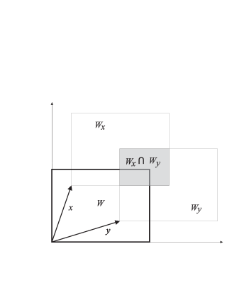
Figure 1: A 2D representation of the denominator in Eq. 12.

from which we have that $\hat{g}_{\rm{STO}}(r)=1+\hat{\xi}_{\rm{STO}}(r)=\hat{\varrho}_{\rm{STO}}(r)/\hat{\lambda}^{2}$. Here $W_{\mathbf{y}}$ denotes the window $W$ shifted by the vector ${\mathbf{y}}$, $W_{\mathbf{y}}=W+{\mathbf{y}}=\{{\mathbf{x}}:{\mathbf{x}}={\mathbf{z}}+{\mathbf{y}},{\mathbf{z}}\in W\}$. The denominator is the volume of the window intersected with a version of the window which has been shifted by the vector ${\mathbf{x}}_{i}-{\mathbf{x}}_{j}$ and it can be written also as $W_{{\mathbf{x}}_{i}}\cap W_{{\mathbf{x}}_{j}}$ (see Fig.1). Clearly, this volume is smaller than the window volume which appears in the naive estimator; thus edge–correction is done.

We want to emphasize here that the point process does not need to be isotropic to get good estimates of $\xi(r)$ through $\hat{\xi}_{\rm{STO}}$, contrary to the four previously mentioned estimators. This property of the $\hat{\xi}_{\rm{STO}}$ estimator makes it very useful, especially when measuring the correlation function in redshift space, because peculiar motions act to erase small scale correlations, flattening thus the shape of the correlation function and providing smaller values for $\gamma$. Beware applying statistics which are not suitable for anisotropic processes, since experience shows that deviations from isotropy may cause great errors if isotropic case estimators are used. In such cases, one can improve the STO estimator by replacing $4\pi r^{2}$ in the denominator of Eq. 14 by the quantity $4\pi|{\mathbf{x}}_{i}-{\mathbf{x}}_{j}|^{2}$.

The estimator $\hat{\xi}_{\rm{STO}}$ uses a smoothing kernel in order to reduce shot noise. The problem of shot noise arises, especially, with DP and HAM estimators because, at small scales, $DR(r)$ becomes very small due to the fact that the number of Poisson points within a shell of radius $r$ is approximately proportional to $r^{2}$. It is worth mentioning that Davis & Peebles (1983) already tried to reduce the shot noise by smoothing $DR(r)$ at small scales ($r<2$ $h^{-1}$ Mpc). Other authors change the estimator used at small scales (van de Weygaert 1991). Other solutions to this problem will be commented in section 5.

There is still another well-known but little appreciated (Blanchard & Alimi 1988) estimator introduced for the study of the angular correlation function by Peebles & Hauser (1974). Its three–dimensional counterpart is

$$\hat{\xi}_{\rm{PH}}=\frac{DD(r)}{RR(r)}\times\left(\frac{N_{\rm{rd}}}{N}\right)^{2}-1.$$ (15)

Peacock (1992) argues that $\hat{\xi}_{\rm{PH}}$ and $\hat{\xi}_{\rm{DP}}$ should be equivalent when applied to a large volume; however the latter is less sensitive to whether there is a rich cluster close to the border of the sample.

It can be shown (Kerscher 1998) that $\hat{\xi}_{\rm{PH}}$ is nothing else than the isotropized Monte Carlo counterpart of $\hat{\xi}_{\rm{STO}}$ in which the smoothing kernel has been substituted by the standard count of pairs $DD(r)$.

The relation between the estimators LS and PH can be easily deduced from their definitions given in Eqs. 6 and 15,

$$\hat{\xi}_{\rm{LS}}=\hat{\xi}_{\rm{PH}}+2-2\left({DR(r)\over RR(r)}\times{N_{\rm rd}\over N}\right).$$ (16)

In a broad sense, most of the estimators consist of a sum of pairs in the numerator whereas the denominator is an edge-corrected version of the denominator in $\varrho^{*}(r)$. The differences among them lie essentially in the way of performing this border correction in the denominator. In cosmology we have to cope most often with complicated windows, so the calculation of $RR$ and $DR$ has to be performed through Monte Carlo integration.

Within this general scheme, RIV presents (at first sight) a certain deviation by summing means of edge-corrected counts of pairs instead of summing the means first and dividing them afterwards like the other estimators do. HAM and STO both present a new approach to the problem: the former arises from minimizing the dependence of the variance on the (not always well known) intensity and the latter introduces a smoothing in the counting of pairs of galaxies.

The estimator $\hat{\varrho}_{\rm{STO}}(r)$ has an irregularity property for small $r$ resulting from the denominator $4\pi r^{2}$. If the numerator of $\hat{\varrho}(r)$ vanishes, then $\hat{\varrho}_{\rm{STO}}(r)=0$ by definition. But if there is at least one pair with a very small interpoint distance then the numerator is positive and $\hat{\varrho}_{\rm{STO}}(r)$ may take a very large value. This problem is discussed in Stoyan and Stoyan (1996). For many point fields this effect does not play a role and it suffices to avoid too small values of $r$. However, in the case of galaxies $\xi(r)$ is known to have a pole at $r=0$ and the multiplicity of this pole is the value of the exponent $\gamma$. Thus small values of $r$ are important and it is precisely in this region where we can observe remarkable differences among the various estimators considered. The set of small $r$ values is not an easy zone to study clustering in because at small distances there are few points and the shot noise dominates; consequently it would be interesting to check if any of the estimators is able to cope at least moderately well with this kind of noise.

On the other hand, in the STO case a contrary effect influences the estimation problem, namely the fact that kernel estimators tend to smooth the results. This may lead to values of $\hat{\varrho}(r)$ which are too low for small $r$. Stoyan and Stoyan (1996) recommend to use large samples and small values of the bandwidth $w$, taking numerical experiments with statistical data from simulated point fields in order to find out the best value; such experiments have led to the result that a good choice of $w$ would be

$$w\equiv c\lambda^{-1/3}\,$$ (17)

with the coefficient $c$ being around 0.1 for point fields such as the Poisson point process. For cluster processes, values of $c$ around 0.05 have yielded acceptable estimates of $\xi(r)$ also for small $r$ and this is the value we use throughout the paper.

3 The estimators acting on galaxy samples

The aim of this Section is to stress the fact that there exists no “perfect estimator” but that, as Doguwa & Upton (1986) remark, the usefulness of an estimator can depend on the kind of process/sample/distance range under study.

3.1 Comparison between DP and HAM

The currently most widely used estimators in the literature are DP and HAM. In this Section we are going to perform a comparison between them by analyzing results of applying them to galaxy samples which have been obtained in different ways.

3.1.1 Complete volume–limited samples

We plot in Fig. 2 the quotient between the Hamilton and the Davis & Peebles estimators of the correlation function for a volume–limited sample extracted from Stromlo-APM, where the values of the correlation functions and of bootstrap errors have been provided to us by J. Loveday. In that case the relative differences are again small and much less significant than the bootstrap errors. In fact this result is used by Loveday et al. (1995) to clarify a possible concern regarding the HAM estimator, showing that it does not remove intrinsic large-scale clustering. So it seems that the main difference between both estimators happens when they are applied to a sample whose density is poorly known, where HAM works better. This is a very sparse sample (only 1 in 20 galaxies from the angular sample is included in the redshift survey), therefore at small scales the statistical quantities are rather noisy. It is interesting to note that the value of $\xi(r)$ at $r=1.23\,h^{-1}$ Mpc is 2.7 for DP and 2.4 for HAM. Although at this scale the error bar is quite large (between 5 and 10), it is clear that the value of $\xi(r)$, assuming it follows a power law, is underestimated by both estimators, indicating a strong bias. At the same scale the RIV estimator provides a larger value for $\xi(r)$, 13.6, which clearly is more acceptable.

3.1.2 Samples with non-uniform density

The expressions we have presented for the estimators are adequate for samples which are either complete or volume–limited. They can be generalized to other kinds of limitation by assigning to each galaxy weights inversely proportional to a certain selection function. This function represents the fraction of the total population of galaxies satisfying the limitation criterion at a certain distance. The weighting scheme used or the uncertainty in the knowledge of the selection function can influence, however, the result for the correlation function. Since we want to compare estimators this added uncertainty would disturb unnecessarily the measure, so we shall mainly work with complete or volume–limited samples.

Nonetheless, we want to show briefly in this subsection an example of the difference of applying DP and HAM to incomplete samples. In particular we have used two samples extracted from the Optical Redshift Survey (described in Santiago et al. 1995), one limited in apparent magnitude and the other in diameter. What we show in Fig. 3 is the quotient between both estimators, i.e., $\hat{\xi}_{\rm{HAM}}/\hat{\xi}_{\rm{DP}}$, calculated by Hermit et al. (1996). The differences are only noticeable at very large scales and they are bigger for the magnitude–limited sample (bottom panel) than for the diameter–limited sample (upper panel). This fact is remarkable because the latter sample is sparser at large distances than the former, since the selection function is steeper for the diameter–limited sample than for the magnitude–limited one (Santiago et al. 1996). However, the Galactic extinction affects galaxy magnitudes more strongly than diameters. The selection function used by Hermit et al. (1986) incorporates an angular dependence modelling the extinction and this fact could explain the deviations observed in Fig. 3. In fact for the Las Campanas redshift survey, having a very complex selection function, Tucker et al. (1997) have shown that, at large scales, the differences between both estimators can be as larger as the signal itself.

3.2 The six estimators acting on a volume–limited sample

Now we shall apply the six mentioned estimators to a complete sample, volume–limited to 79$h^{-1}$ Mpc, extracted from the Perseus-Pisces Survey (for a thorough description of the sample, see Kerscher et al. 1997). The results can be observed in Fig. 4 and show that, at small and intermediate scale, all estimators behave similarly except STO, which gives a bigger value of $g$; as we shall later see, this estimator has a smaller variance than the others at small scales, important for the determination of $\gamma$. This can be interpreted saying that its nature makes it less sensitive to local anisotropies due to peculiar motions. This result mainly indicates that all the estimators measure the two-point correlation function rather well in the “easy” range $2<r<15$$h^{-1}$ Mpc. For bigger scales, relevant for information on a possible trend to homogeneity of the matter distribution, there are some differences as well. Therefore, it is worth to study the behaviour of the different estimators on controllable point sets in order to know the deviation of each one from the true value of the two-point correlation function and the ensemble variance. The test performed in Section 5 points in this direction.

4 Description of the artificial samples

4.1 Cox processes

We shall make use of an artificial sample which is a particular kind of a so-called segment Cox point process. This is a clustering process for which an analytical expression of its 2–point correlation function is known and therefore can be used as a test to check the accuracy of the $\xi$–estimators. The variant we are going to use is produced in the following way: segments of length $l$ are randomly scattered inside a cube $W$ (see Fig. 5) and on these segments points are randomly distributed. Let $L_{V}$ be the length density of the system of segments, $L_{V}=\lambda_{\rm{s}}l$, where $\lambda_{\rm{s}}$ is the mean number of segments per unit volume. If $\lambda_{l}$ is the mean number of points on a segment per unit length, then the intensity $\lambda$ of the resulting point process is

$$\lambda=\lambda_{l}L_{V}=\lambda_{l}\lambda_{\rm{s}}l\,.$$ (18)

For this point field the correlation function can be easily calculated taking into account that the point field has a driving random measure equal to the random length measure of the system of segments. Stoyan, Kendall and Mecke (1995) have shown that the pair correlation function of the point field equals the pair correlation function of the system of segments, which reads

$$\xi_{\rm{Cox}}(r)=\frac{1}{2\pi r^{2}L_{V}}-\frac{1}{2\pi rlL_{V}}$$ (19)

for $r\leq l$ and vanishes for larger $r$. As we can see, the expression is independent of the intensity $\lambda_{l}$.

In Section 5.2 we shall use 10 realizations of a segment Cox process generated inside a cube of sidelength $L=100$ $h^{-1}$ Mpc with values of the parameters $\lambda_{\rm{s}}=10^{-3},\lambda_{\rm{l}}=0.6$, and $l=10$ $h^{-1}$ Mpc, which produces sets containing $N\simeq 6000$ points.

4.2 Simulated galaxies

In this subsection we show how a sample of synthetic galaxies was obtained from a simulation of a CDM–type Universe. The cubic region modeled was of sidelength 80$h^{-1}$ Mpc, a standard $\Omega=1$ Universe was chosen, and the initial computational grid was 32³, with the same number of particles. The run started from small perturbation amplitudes and was terminated when the $\sigma_{8}$ parameter, the mass dispersion in 8$h^{-1}$ Mpc radius spheres, was close to the observed value 1. We used H. Couchman’s public domain adaptive P³M code (which can be obtained at http://coho.astro.uwo.ca/pub/ap3m/ap3m.html), and the initial data were those of the test model supplied with this code. The initial density perturbation spectrum was close to the observed one for scales of 8–10$h^{-1}$ Mpc with a rather sharp cutoff used to eliminate numerical effects:

$$P(k)\sim k^{-1}\exp(-(k/k_{c})^{16}).$$ (20)

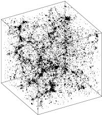
Figure 6: Density distribution for the P³M model.

The cutoff wavenumber $k_{c}=0.96h$Mpc^-1 is lower than the Nyquist frequency used in the computations (with a 32³ grid the smallest usable wavelength is 5$h^{-1}$ Mpc, while the cutoff wavelength is 6.5$h^{-1}$ Mpc). The final state of the model represents a continuous distribution of dark matter in the computational volume (see Fig. 6).

In order to get closer to observations one has to predict the positions of luminous objects (galaxies, their groups or clusters) on the basis of this distribution. There exist many essentially phenomenological methods for doing this, and we have applied another one, the recent equal–mass binary tree approach. These trees are known as multidimensional $k$-trees; they were used first in the statistics of cosmological data by van de Weygaert (1988) and have now been resurrected by Suisalu et al. (1999), who give in that paper the detailed description of their motivation and of the intricacies of their use. The present application is ideal for these trees, having a perfectly shaped volume and a number of particles that is a power of 2.

The equal–mass trees are constructed by dividing the sample volume successively into smaller subvolumes, keeping the mass (number of points) of the two subvolumes equal. In order to illustrate the method, we show in Fig. 7 how a planar point process with $2^{4}$ points is divided by means of the equal–mass tree for the two different starting directions.

This procedure assigns a fixed mass to a given level of subdivision, while the values of the subvolumes and their positions describe the density distribution for a given mass scale. One can select objects applying either a mass or a density bias and we choose the latter. In other words, for a given level of subdivision all cells have the same mass, but different density. The density is just proportional to the inverse of the volume of the cell. The mass within a cell will form a galaxy if its density exceeds a given threshold. We have applied this procedure to the CDM simulation. In Fig. 8 we have plotted the number of cells $N$ with density exceeding a given density threshold $n$ for each level $l$ of subdivision. It can be seen that the isolevel lines split into three, showing the scatter for trees that have different starting directions.

For the present study we used samples selected on the basis of a fixed threshold density, $n=10^{6}$ (in units of number of points divided by the fraction of the whole volume occupied by the cell), and for four levels. Each level can be assigned a fixed mass, $M_{\ell}=1.4\times 10^{17}h^{-1}2^{-\ell}M_{\odot}$. The mass range for our samples runs from $4.3\times 10^{12}h^{-1}M_{\odot}$ for the finest subdivision, somewhat higher than the total mass of a giant galaxy, to $3.4\times 10^{13}h^{-1}M_{\odot}$, characteristic for a group or a poor cluster of galaxies. Each object gets its coordinates from the centre of the cell that collapsed to form it, and we used a fixed starting direction to construct a tree.

The spatial distribution of the objects of our samples is shown on the left side of Fig. 9. From top to bottom the panels correspond to levels $\ell=12,13,14,15$ and the number of points of each subsample is respectively $N=762,1930,4734,11284$. As it can be seen, the geometry of the mass distribution for different mass levels does not differ much.

5 Comparison of the estimators of the correlation function

5.1 Dependence on $N$

We have calculated the pair correlation function $g(r)=1+\xi(r)$ for the four samples shown in Fig. 9 by means of four of the estimators described in Section 2. Our aim was to check the influence of the total number of points $N$ on each of them. The extracted galaxies we have described in Section 4.2 are appropriate for this check because these samples trace the same structure with increasing number of points for bigger levels $\ell$.

The results are shown in the right panels of Fig. 9. We can see that at large scales there is full agreement among the four methods but, at short distances, STO and RIV still agree rather well, while DP and HAM deviate from this behaviour. In all cases we have used random realizations containing $N_{\rm{rd}}=20000$ points each. This is a typical number of random points used in the computation of $\xi(r)$ (Dalton et al. 1994, Tucker et al. 1997). We see in the plot that the relation among the different estimators remains similar from one panel to the other although $N$ is varying by a factor 15 in total.

The conclusion is that $N$, provided it is big enough to trace satisfactorily the main structures present in the sample, does not have a significant influence on the estimation of the correlation function.

We have repeated this analysis by using the same data sample ($\ell$ =12, $N=762$ simulated galaxies), but different realizations of random samples (different seeds). For $10^{4}$ random points the differences in correlation functions were appreciable for all four estimators that use auxiliar random samples, but for $10^{5}$ points the correlation functions practically coincided, except for small $r$ values for DP and HAM. In next subsection we study in more detail the dependence on $N_{\rm{rd}}$ by means of the Cox processes.

5.2 Dependence on $N_{\rm{rd}}$

First we have performed a couple of tests on 10 Cox processes of the kind described in Section 4.1, consisting in calculating for them $\xi$ and the ensemble error with the four estimators introduced in Section 2 depending on $N_{\rm{rd}}$. We see in Fig. 10 what happens when we increase the number of random points: $10^{4},10^{5},10^{6}$. Our aim is to check if the value of $N_{\rm{rd}}$ is the source of the differences among them. In Fig. 10 the results of $\xi$ for very small distances have been suppressed since the use of Poisson samples introduces shot noise in the estimators because the local fluctuations become important. One sees that increasing the number of random points helps reducing the variances, but of course for using a very large number of random points, one has to resort to efficient searching algorithms like those based on the multidimensional binary tree (Martínez et al. 1990) to count the number of pairs $RR(r)$ and $DR(r)$. Alternatively, one has to use analytical expressions for the evaluation of these quantities (see the appendix in Hamilton (1993)).

Except for the first bin in DP and HAM, the results are practically the same using $N_{\rm{rd}}=10^{5}$ than using $N_{\rm{rd}}=10^{6}$; that means that, for this process and choice of parameters, $N_{\rm{rd}}=10^{5}$ is “big enough”. Let us notice that in this case the difference between PH and LS is very small, tending to 0 as $N_{\rm{rd}}$ increases, since then $(DR(r)/RR(r))\times(N_{\rm rd}/N)$ tends to 1 (see Eq. 14).

As we can see, DP and HAM estimators have a larger scatter for the correlation function at short distances than do PH and LS. This is due to the fact that the shot noise acts to create spurious clustering in the random samples at small distances, influencing the computational number of pairs $DR(r)$ and $RR(r)$ and through those the estimators HAM and DP. The bigger problem is $DR(r)$ which does not enter in the estimator PH. If one wishes to use $DR(r)$ as a background number of pairs to normalize the quantity $DD(r)$, one has to use a large enough random sample in order to make the fluctuations negligible. But, how large? The intensity (number density) of the random sample should be at least that of the local intensity of the real catalog in the clustered regions. For example, for the segment Cox processes used here, we deduce a priori the number of random points needed to estimate reliably $\xi(r)$ at small separations. From the expression of the correlation function given in Eq. 19, we know that for this kind of process the average density at a distance 0.3 $h^{-1}$ Mpc of a given point is 172.5 times the mean number density, $6\times 10^{-3}$; therefore if we want to map these distances with the random sample, we need at least $\sim 10^{6}$ random points in order that the intensity of the random catalog equals the previous value of the local density. At this point it is interesting to remark that at the smallest interpoint separations, the effects of the finite boundaries on the estimates of $\xi(r)$ are less important than at large scales; however it is more difficult to cope with them with this kind of estimators, because one needs to use a huge amount of random points or other sophisticated solutions to get reliable results.

Another practical rule to decide if the random catalogue used is large enough is to repeat the calculations using different random seeds – if the results differ appreciably in the region of interest, then it is necessary to increase the size of the random sample (or to choose another estimator).

At intermediate scale all the estimators give the right result with moderate error bars whereas at large scales the errors increase for all estimators. Therefore, the difficulty to obtain accurate estimates of $\xi$ at big distances does not seem to be only due to the form of a particular estimator or to the number of random points used but to the statistic itself. Note, however that we have limited our analysis to scales $r\leq l$; at the end of Section 5.4 we will compare some estimators at longer distances by means of simulations of the cluster distribution.

5.3 Estimation of biases

We shall now consider the results of the previous subsection for the biggest $N_{\rm{rd}}$ used. Although, as we have seen, increasing $N_{\rm{rd}}$ reduces the variances, the same effect is not found for the bias. We shall proceed to plot in Fig. 11 a measure of the bias in the form of a quotient between the mean of the 10 estimated values of $g$ for each estimator using $N_{\rm{rd}}=10^{6}$, and the theoretical $g_{\rm{Cox}}$. We want also to include for the comparison the STO and RIV estimators. We shall estimate the volumes entering their definition by means of analytical expressions which are available for this simple geometry.

At distances $r\geq 2$$h^{-1}$ Mpc the biases of all the methods are of the same order and the results for $g(r)$ are quite reliable when compared with the expected theoretical values given in Eq. 19. At short distances the estimator STO performs very well providing the smallest bias. This good performance is probably related with the fact that the segment Cox process is at small scales locally anisotropic (points randomly placed on a segment) and as we have explained the STO estimator deals well with this kind of process. The other estimators show a clear bias at small scales, underestimating the true value of the correlation function. It is expected that for very large windows and a large number of points in the point sample all estimators are of a similar quality (Hermit et al. 1996).

5.4 Variance at large scales

The variance for an estimator on a Cox process could be different from that of the same estimator applied to galaxy catalogues or cosmological simulations. Moreover, the kind of Cox process used here has a limitation due to the finite length of the segment employed to generate the point distribution, namely that $\xi$ vanishes for a distance greater than that length. In order to see what happens in the absence of such limitation we have taken 10 CDM cluster simulations produced by Croft & Efstathiou (1994) and calculated $g$ on them using the six estimators. The results of their standard deviation show in Fig. 12 that, at large scale, HAM and LS have a smaller variance than the others, which could not have been appreciated in the Cox processes where we should not go farther than 10$h^{-1}$ Mpc in distance. This result supports Hamilton’s claim that the estimator proposed by him (Hamilton 1993) is more reliable on large scales, where the correlation function is small. Its use provides interesting clues on the transition to homogeneity of the galaxy distribution at large scales (Martínez, 1999). Other tests have been performed on simulations for which $g(r)=1$ at large scales. For these simulations, Hamilton’s estimator has a small systematic bias but a very little estimation variance. Combining both quantities in the square deviation of the true value, HAM shows a large degree of precision at large scales. The reason for that lies in the fact that the term $DR(r)$ in Eq. 5 is related to an improvement of the estimator of the intensity (Stoyan & Stoyan 1998).

6 Estimation of errors using Cox processes

After having performed the previous tests, we are now ready to use Cox processes for estimating errors. We shall do it on the extracted galaxy sample corresponding to the $\ell=12$ level but the method would be analogous in the other cases.

As Hamilton (1993) points out (see references therein), five methods of estimating the variance of $\xi$ are commonly used: Poissonian error, idem enhanced by a certain factor, bootstrap, ensemble error coming from calculating $\xi$ in subregions of the sample and, finally, ensemble error coming from artificial samples suffering the same selection effects than the real sample. The kind of error we are going to give belongs to the fifth group.

We simulate 10 Cox segment point fields with the following values of the parameters $l=20$ and $\lambda_{\rm{s}}=4\times 10^{-5}$. This leads to a correlation function which is comparable with the 2–point correlation function of the sample of simulated galaxies stopping at the $\ell=12$ level described in Section 4.2 and which approximately verifies $\xi(20)=0$ and $\xi(10)=1$. Typically these point fields will be generated inside a cube of 80$h^{-1}$ Mpc sidelength containing about 800 points. Using similar kind of processes (objects homogeneously distributed in filaments and sheets), Buryak & Doroshkevich (1996) have simulated the galaxy distribution.

As can be appreciated in the plots of Fig. 9, the use of different estimators causes variability in the slopes of the correlation function. A least squares fit to a power–law for $g(r)\simeq r^{-\gamma}$ in the range [0.5,8] $h^{-1}$ Mpc gives the following results for four of the methods: $\gamma_{\rm{DP}}=2.14\pm 0.06$, $\gamma_{\rm{HAM}}=2.27\pm 0.09$, $\gamma_{\rm{RIV}}=2.03\pm 0.04$, $\gamma_{\rm{STO}}=2.03\pm 0.04$ for a true value $\gamma\simeq 2$ due to the shape of the power–spectrum (Eq. 20). The fit has been performed using linear bins and the value of $\hat{g}$ in a particular bin has been assigned to its centre. In this case the error accompanying the previous numbers comes from the weighted least squares fit taking as errors for $g(r)$ the ones obtained using the Cox processes mentioned in the previous paragraph.

Apart from using these simulations to test the stability of the methods, we want to stress that this is a way to evaluate the errors of the correlation function for a given realization, alternative to the standard bootstrap. Let us stress the idea of the method, which is similar to measuring the dispersion of $\xi$ in ensembles of many independent synthetic catalogues with similar statistical properties (Fisher et al. 1993): we use cluster point processes with the same intensity as our sample and with a known analytical expression for $\xi(r)$, we build a model having similar correlation behaviour to that of our galaxy sample, i. e., a similar $\xi(r)$ in the whole range of scales, and then we are able to estimate the ensemble error by constructing several realizations of the point process, applying the estimator of $\xi$ to all these realizations and measuring the standard deviation. We believe that this method for the estimation of the errors is more reliable than the standard bootstrap because of a serious conceptual weakness the latter suffers from, namely that the bootstrap suggested in Ling et al. (1986) produces new point patterns by sampling with replacement; consequently, in each new point pattern there are multiple points, i.e., quite heavy clusters. In cluster point processes the degree of clustering will increase. This leads to incorrect, probably too great, error predictions. Fisher et al. (1994) show how bootstrap errors are in general an overestimate of the true errors.

7 Conclusions

In this paper we have performed a comparison, by using Cox processes, of most of the existing 2–point correlation function estimators.

We would like to point out that a clear distinction has to be made among the statistical quantity $\xi(r)$, the estimator used to evaluate it on a particular galaxy catalog, $\hat{\xi}(r)$, and the particular algorithm of computation of the quantities entering into the estimator. It is important to note that what we have compared here is the performance of different estimators, each implemented in its simplest way, following the definitions given in Section 2. These kinds of implementations are the ones commonly used in Cosmology. In particular, the estimators depending on the background pair counts $RR(r)$ and $DR(r)$ need a large amount of random points $N_{\rm{rd}}\sim 10^{6}$ if one is trying to accurately measure the correlation function at the smallest separations, although good enough results can be obtained at medium and large scales with $N_{\rm{rd}}\sim 20000$. Note that these figures are appropriate for samples with this density but that, for samples with other characteristics, one should previously perform tests in order to decide which is a good value for $N_{\rm{rd}}$. Cox processes are a good benchmark for such tests. The results show that at large distances all estimators present similar values and big errors with HAM and LS clearly being better than the others, at intermediate distances values and errors are similar and perfectly acceptable, and at short distances the errors for STO are clearly the smallest. Note, however, that the variance of the former gets smaller by increasing the number of random points or using alternative ways for accurately estimating the number of background pairs. Another advantage of RIV and STO is that they compute something as easy to accurately estimate as volumes (in the Monte Carlo implementation the dependence on $N_{\rm{rd}}$ is softer than for the others because the random points are being used only for the evaluation of volumes and not for computation of pairs), whereas in order to increase accuracy in the others one should make use of a “big enough” random sample and the decision about how big that should be, in the absence of previous numerical tests, is somewhat arbitrary. Unfortunately one factor of arbitrariness is always present, namely the length of the bin in distance (or the coefficient $c$ in the choice of bandwidth for STO estimator).

The main conclusion we have drawn from our analysis is that there exists no optimal estimator but that each one has advantages and weak points and, depending on the nuances of the problem we want to analyze, one or another will be preferable. In the case of complete samples limited in volume, RIV is not very sensitive to the number of random points used to evaluate the volumes but presents a bias at small distances; HAM has small variance at long distances but larger at small distances and in this range is highly sensitive to $N_{\rm{rd}}$ and it is biased; DP has a big variance and presents a bias at short scales; PH depends also on $N_{\rm{rd}}$ but less than HAM and DP and also shows a bias at small scales; STO is never the worst in any of the tests and can be applied also to anisotropic processes; and LS behaves in many aspects similarly to PH but with a smaller variance at large scale. For samples with non-uniform density these conclusions may vary, and in particular HAM is preferable at large scales.

Two further points—secondary with regard to the comparison of estimators but also interesting and potentially useful for researchers on this field—have been treated: for testing the estimators we have introduced a new phenomenological method to extract galaxy samples from cosmological simulations based on the multidimensional binary trees; and, for such samples, we have estimated errors in the determination of the 2–point correlation function by using realizations of a Cox process with the same number density as the simulated sample.

Figure 2: The quotient between the Hamilton and Davis & Peebles estimators for the correlation function of a volume–limited sample extracted from the Stromlo-APM redshift survey.

Figure 3: The quotient between the Hamilton and Davis & Peebles estimators for the correlation function of samples extracted from the Optical Redshift Survey (top: diameter–limited and bottom: magnitude–limited).

Figure 4: The correlation function of the PPS sample calculated by means of the six estimators described in Section 2.

Figure 5: Simulation of the Cox process with $N=6007$ points.

Figure 7: Dividing up a surface keeping equal mass in each cell at a given level. Different levels are represented with different line styles. Each panel shows the division with different starting direction.

Figure 8: Number of objects for a given level and density threshold.

Figure 9: Letf panels: spatial distributions of galaxies drawn from a CDM simulation by means of the multidimensional binary tree. Right panels: The corresponding function $g(r)$ for the four samples calculated by means of four of the methods: dotted line (Davis & Peebles), dashed-dotted line (Hamilton), dashed line (Rivolo) and solid line (Stoyan & Stoyan)

Figure 10: 2–point correlation function and standard deviation when calculated on 10 realizations of a Cox process for the estimator and number of random points indicated in each panel. The continuous line corresponds to the analytical $\xi_{\rm{Cox}}$ (Eq. 17).

Figure 11: Ratio between the mean of $\hat{g}$ and $g_{\rm{Cox}}$, for each estimator, calculated on 10 Cox processes using an auxiliary random sample containing $N_{\rm{rd}}=10^{6}$ points.

Figure 12: Standard deviation of the six estimators when applied to a set of 10 CDM cluster simulations.