MAKING SENSE OF SUNSPOT DECAY

Abstract

In a statistical analysis of Debrecen Photoheliographic Results sunspot area data we find that the logarithmic deviation $(\log D)^{\prime}$ of the area decay rate $D$ from the parabolic mean decay law (derived in the first paper in this series) follows a Gaussian probability distribution. As a consequence, the actual decay rate $D$ and the time-averaged decay rate $\overline{D}$ are also characterized by approximately lognormal distributions, as found in an earlier work. The correlation time of $(\log D)^{\prime}$ is about 3 days. We find a significant physical anticorrelation between $(\log D)^{\prime}$ and the amount of plage magnetic flux of the same polarity in an annulus around the spot on Kitt Peak magnetograms. The anticorrelation is interpreted in terms of a generalization of the turbulent erosion model of sunspot decay to the case when the flux tube is embedded in a preexisting homogeneous “plage” field. The decay rate is found to depend inversely on the value of this plage field, the relation being very close to logarithmic, i.e. the plage field acts as multiplicative noise in the decay process. A Gaussian probability distribution of the field strength in the surrounding plage will then naturally lead to a lognormal distribution of the decay rates, as observed. It is thus suggested that, beside other multiplicative noise sources, the environmental effect of surrounding plage fields is a major factor in the origin of lognormally distributed large random deviations from the mean law in the sunspot decay rates.

1 Introduction

The very large and apparently random individual differences in the area decay rates of sunspots have constituted a serious obstacle in the way of an empirical determination of a mean decay law. With time it has been recognized that the study of the distribution of decay rates itself may be of key importance for the proper statistical analysis of the decay, as most of the widely applied tools of mathematical statistics (e.g. least-square fits) are based on the tacit assumption of one particular (usually the Gaussian) probability distribution. The realization that the mean area decay rates $\overline{D}$ of sunspots are distributed lognormally (Martínez Pillet, Moreno-Insertis, and Vázquez, 1993, hereafter MMV93) was therefore an important step towards the proper understanding of the statistical regularities underlying the apparently haphazard sunspot decay process. A lognormal distribution implies that it is the logarithm of the decay rate $D$ that is normally distributed, and thus it is $\log D$ that should be used as the dependent variable in least-square fits and other standard statistical procedures. This realization has helped us in the first paper of this series (Petrovay and van Driel-Gesztelyi, 1997, hereafter Paper I; see also Petrovay, 1998) to finally determine, by rigorous statistical methods and at a quite convincing confidence level, the mean law governing sunspot decay. It was found that an “idealized” sunspot following this mean law exactly, with no random deviations, would decay according to the law

$$D_{\mbox{\scriptsize ideal}}=C_{D}\,r/r_{0}\qquad C_{D}=32.0\pm 0.26.$$ (1)

where $D_{\mbox{\scriptsize ideal}}$ is the area decay rate $D$ for an idealized spot in units of MSH/day (MSH: one millionth solar hemisphere), $r$ is the equivalent radius of the spot (i.e. the radius of the circle with the same area as that of the spot), while $r_{0}$ is its maximal equivalent radius. (The corresponding areas will be denoted by $A$ and $A_{0}$, respectively.) It is clear that as $D=-\dot{A}$ and $r\sim A^{1/2}$, Equation (1) implies a parabolic decrease of the spot area with time, in contrast to the previously widely held view that the decay is linear.

For real spots the actual daily decay rate $D$ shows random deviations from the law (1). It follows from the considerations of the first paragraph above that in the derivation of the law (1) it is the logarithm of $D$ that had to be averaged, i.e. the mean decay law for real sunspots is

$$\langle\log D\rangle=\log(C_{D}\,r/r_{0})$$ (2)

(Here we are using the notation $\langle a\rangle$ for the ensemble average over many spots at the same phase of decay $r/r_{0}$, as opposed to the time average over the decay phase of one spot, $\overline{a}$. Deviations from the ensemble average are denoted as $a^{\prime}=a-\langle a\rangle$.)

Having determined the mean decay law, in the present paper we turn our attention to the deviations from this mean law. There are several important issues to clarify in this respect.

• The analysis of Paper I assumed that $(\log D)^{\prime}$ follows a Gaussian distribution. In the case of a parabolic decay law like (1) however it is not possible to have a strictly normal distribution simultaneously for $(\log D)^{\prime}$, and also for $\log\overline{D}$ and $\log D$, as suggested in MMV93. In Section 2 we therefore consider the question, which one of the proposed lognormal distributions is the fundamental and exact one, and which are those that are only approximate and appear as secondary consequences of the fundamental distribution.

• The decay law (1) implies that the decay process has a “memory”: in order to “know” the “right” decay rate, the spot must remember its maximal radius $r_{0}$ at all later phases of its decay. The question arises, how can this long-term memory be reconciled with the presence of random fluctuations in the decay rate? In Section 3 we first estimate the correlation time of the fluctuations, and then, considering the possible explanations, we conclude that the “memory” responsible for both the long-term systematics and for the short-term fluctuations can be identified with the amount of flux stored in the plage around the spot. This implies that decay rate fluctuations should be correlated with the amount of this flux.

• In order to check the above prediction, in Section 4 we compare the amount of magnetic flux in an annulus surrounding the spot, as determined from Kitt Peak magnetograms, with the decay rate. We indeed find a significant anticorrelation between the two quantities. Interpreting this empirical anticorrelation, in Section 5 we generalize the turbulent erosion model to account for a plage field.

Finally, in the Conclusion we discuss and summarize the main factors leading to, and the physical interpretation of the fluctuation in the decay rates.

Throughout the paper, we use the same data set as in Paper I, taken from the Debrecen Photoheliographic Results (DPR) 1977–78 (Dezső, Gerlei, and Kovács, 1987, 1996). This consisted of 3990 area measurements of 476 different spots. For a detailed discussion of the data selection and reduction process we refer the reader to Section 3 of Paper I. In order to extend the data set, we made an attempt to include data from the more extensive Mt Wilson catalogue. However, owing to the lower precision of those data and the problems with the day-to-day identification of sunspots we decided to use the DPR data only for the present analysis. Nevertheless, the comparison of the two catalogues offered some interesting conclusions, summarized in Appendix A.

2 The distribution of decay rate fluctuations

Figure 1a shows the histogram of $(\log D)^{\prime}$, as defined after Equation (2), for our sample (dash-dotted line). This original histogram is distorted by the selection effect described in Section 3.3.2 of Paper I: this effect essentially consists of a lower expected number of observations for spots with higher decay rates, and thus shorter lifetimes. (The histogram contains data points with $r/r_{0}>0.7$ only, to avoid the regime most affected by this bias.) Correcting for the bias using the method described there, we obtain the histogram shown by the solid line. A Gaussian fit to this histogram (dashed) is found to be a fairly good representation of the data. ($Q=\Gamma[(N-1)/2,\chi^{2}/2]=0.02$; the skewness and kurtosis are $-0.20\pm 0.21$ and $0.67\pm 0.52$, respectively, i.e. not significantly different from 0.) This normal distribution of $(\log D)^{\prime}$ confirms the correctness of the analysis of Paper I, based on least-square fits with $\log D$ as the dependent variable.

Figure 1: Histograms of (a) $(\log D)^{\prime}$ and (b) $\log D$ for all spots that died on the visible hemisphere. (Fig. 1a contains data for $r/r_{0}>0.7$ only.) Dash-dotted: raw histograms; solid: histograms corrected for selection effect; dashed: Gaussian fits. The parameters of the fits are $\langle{(\log D)^{\prime}}\rangle=-0.09$, $\sigma=0.19$ for (a) and $\langle{\log D}\rangle=1.25$, $\sigma=0.23$ for (b).

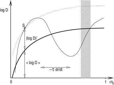
Figure 2: Sketch for the explanation of the relation between the lognormal distributions of different decay rates. $S$ is a generic data point in the plane $r/r_{0}$–$\log D$ where the thick curve represents the mean decay law (1). The thin curve is a decay curve for a generic sunspot with a random logarithmic deviation $(\log D)^{\prime}$ varying on a timescale $\tau$, while the dotted curve is the decay curve of a hypothetical suspot with a constant logarithmic deviation from the mean law, $(\log D)^{\prime}=$const.

In MMV93 it was found that, within the errors, $\log\overline{D}$ is normally distributed. Furthermore, based on a statistics of Mt Wilson data (Howard, 1992) it was suggested that $\log D$ should also show a Gaussian distribution. However, our above finding on the normal distribution of $(\log D)^{\prime}$, together with the parabolic mean decay law (2), implies that the distributions studied in MMV93 cannot be exactly Gaussian.

To see this first for $\log D\equiv\langle\log D\rangle+(\log D)^{\prime}$, let us consider the plane $r/r_{0}$–$\log D$ (Figure 2). The normal distribution of $(\log D)^{\prime}$ with zero mean implies that, for a narrow range of $r/r_{0}$ (shaded area), $\log D$ is also normally distributed around a mean value $\log(C_{D}r/r_{0})$. This mean depends on $r/r_{0}$; hence, the distribution of $\log D$ in the complete sample (essentially, the distribution of all data points in the plane projected on the ordinate) will deviate from a Gaussian. (This is in contrast to the case of linear decay where the mean decay law, indicated by the thick curve on Figure 2, would be a horizontal line, independent of $r/r_{0}$.) Indeed, in Figure 1b we present the histogram of $\log D$: while at first glance the quality of the fit does not seem to be very different from the previous case, a quantitative analysis shows that the Gaussian fit is insufficient to explain the data. ($Q<10^{-5}$; the skewness and kurtosis are $-0.77\pm 0.13$ and $-0.13\pm 0.33$, respectively, i.e.  the skewness significantly differs from 0.) The deviation from gaussianity is relatively mild owing to the fact that the number of data points is higher for higher values of $r/r_{0}$ (cf. Fig. 1 of Paper I) where the thick curve representing the mean law is not far from horizontal. The distribution of $\log D$ is therefore indeed approximately lognormal, as proposed in MMV93; but, as we pointed out, the deviation is statistically significant.

Let us now turn our attention to the time-averaged decay rate, defined as

$$\overline{D}=\frac{1}{t_{2}-t_{1}}\int_{t_{1}}^{t_{2}}D\,dt.$$ (3)

Defining $\log C_{D}^{\prime}\equiv\log C_{D}+(\log D)^{\prime}$, according to Equation (2) we may formally write

$$D=C_{D}^{\prime}r/r_{0}.$$ (4)

For a hypotetical sunspot with $(\log D)^{\prime}=$const. (dotted curve in Figure 2) $C_{D}^{\prime}=$const., so from Equation (4)

$$\log\overline{D}=\log C_{D}^{\prime}+\log\overline{r/r_{0}}$$ (5)

where the last term is a constant for all spots, as for a parabolic decay law, $r$ decreases linearly with time. ($\overline{r/r_{0}}=0.5$ if $t_{1}$ and $t_{2}$ correspond to the area maximum and the total disappearance of the spot, respectively.) So for such spots if $(\log D)^{\prime}$ is normally distributed, so is $\log C_{D}^{\prime}$ and $\log\overline{D}$. For real sunspots, however, $(\log D)^{\prime}$=const. does not apply; instead, their actual decay rate will fluctuate around the mean law with some timescale $\tau$ (thin curve in Figure 2), and the above reasoning does not hold. Note that if the mean decay law were linear ($\langle\log D\rangle=$const.), the resulting distribution of $\log\overline{D}$ would still be normal, albeit with a lower dispersion $\sigma$, as in that case the last term in Equation (5) would not be present.

Thus, $\overline{D}$ in general cannot be exactly lognormally distributed; but its actual distribution may still appear to be close to lognormal provided either that $(\log D)^{\prime}$ does not change very much in the time interval $[t_{1},t_{2}]$ (i.e. that $t_{2}-t_{1}<\tau$) for the majority of spots in the sample, or that $r/r_{0}$ does not change very much in the same time interval so that the mean decay rate may be considered nearly constant in that period of time.

For a time average taken over the whole decay phase, $t_{1}$ should be the time of area maximum, and $t_{2}$ the end of the life of the spot. The number of spots in our sample for which both their birth and death were observed is, however, insufficient for a precise empirical determination of the distribution of $\log\overline{D}$.

One way to increase the number of spots in the sample is to define $t_{1}$ and $t_{2}$ as simply the first and last observations of a given spot, without respect to whether these coincide with the birth/death of the spot. However, we have just seen that for the departure from a Gaussian distribution to be significant it is important that we have $t_{2}-t_{1}>\tau$ where $\tau$ is the correlation time of decay rate fluctuations and that $r/r_{0}$ take a sufficiently wide range of values during the observation period. As these conditions are only valid for a relatively low fraction of all spots, the overall distribution derived in this manner may be expected to stay quite close to Gaussian. This may explain the findings of MMV93, where the method applied to determine $\overline{D}$ was indeed crudely the same as outlined in this paragraph.

We therefore conclude that the probability distribution of $(\log D)^{\prime}$ is close to normal, and we propose that it is this distribution that should be considered as fundamental both in a physical and in a mathematical sense. The approximately (but not exactly) Gaussian character of the distributions of $\log D$ and $\log\overline{D}$ is then a secondary consequence of that fundamental distribution.

Figure 3: Autocorrelation of $(\log D)^{\prime}$ for sets of data pairs of different mean time separation.

3 The memories of a sunspot

Figure 3 presents the autocorrelation of $(\log D)^{\prime}$ for sets of data pairs of different mean time separation (data pairs separated by 1,2,3,$\dots$ consecutive observations) . It is apparent that the autocorrelation time (where the autocorrelation sinks below $1/e$) is crudely $\sim 3^{\mbox{\scriptsize d}}$, to be compared with a typical spot lifetime of $\sim 7^{\mbox{\scriptsize d}}$ in our sample. (This latter typical lifetime is entirely due to selection effects, but this is irrelevant for the present argument.)

The existence of random time-dependent fluctuations in the decay rate with a correlation time shorter than the typical lifetime of spots leads to an apparent conceptual problem. As already mentioned in the Introduction, the mean decay law (1) has a curious property: it implies that sunspots have some “long-term memory” of their maximal radius even towards the end of their lives. Two small sunspots of identical size will have different expected daily decay rates if their maximal sizes were different. But if the decay process is subject to a random “noise” with a short correlation time, how is it possible for it to still possess a long-term “memory” in a statistical sense?

The turbulent erosion model of sunspot decay (Petrovay and Moreno-Insertis, 1997, hereafter PM97) successfully predicted the law (1). In this model a “memory” effect is present due to the magnetic flux lost from the flux tube and piled up in its surroundings. The amount of this flux will influence the steepness of the field gradient just outside the current sheet (CS), which in turn determines the propagation speed of the CS (cf. Equation (10) in PM97). Thus, in the framework of this model any fluctuations in the decay rate must be due to fluctuations in the amount of the flux outside the tube. This flux can be considered the sum of two contributions:

$$\Phi=\Phi_{\mbox{\scriptsize lost}}+\Phi_{\mbox{\scriptsize plage}}$$ (6)

where $\Phi_{\mbox{\scriptsize lost}}$ is the flux lost from the spot, while $\Phi_{\mbox{\scriptsize plage}}$ is the flux of independent origin. This latter contribution is partly due to plage fields $\Phi_{\mbox{\scriptsize pl,0}}$ which are originally present in the area, and partly to plage fields $\Phi_{\mbox{\scriptsize pl}}^{\prime}$ which are carried into/out of the neighbourhood of the flux tube by horizontal flows, flux loss from other spots, and so on:

$$\Phi_{\mbox{\scriptsize plage}}=\Phi_{\mbox{\scriptsize pl,0}}+\Phi_{\mbox{\scriptsize pl}}^{\prime}$$ (7)

Both terms in Equation (6) show random fluctuations in time. Now averaging the equation we obviously have a relation for the expected value of the flux around the spot (and therefore for the expected value of the decay rate) as a functional of the mean decay law (first term on the r.h.s. of Equation (6)) and as a function of the plage flux $\Phi_{\mbox{\scriptsize pl,0}}$ originally present in the site of the spot (second term; the other contributions $\Phi_{\mbox{\scriptsize pl}}^{\prime}$ to this term can be supposed to have zero mean). Specifically, if $\Phi_{\mbox{\scriptsize plage}}=0$, we are back to the models presented in PM97; the more general case will be treated in Section 5 below. The initial conditions thus fully determine the expected value of $D$ at any later time. It is thus possible to have a long-term“memory” in the statistical sense while short-term fluctuations are still present.

Clearly, the above reasoning also identifies a main physical factor contributing to the fluctuations in $D$: the ever-changing plage fields in the neighbourhood of the spot. Indeed, within the framework of the erosion model this is the only possible reason for deviations from the mean law. In reality, other contributions may originate in departures from the conditions of the erosion model (i.e. from depth-independence and axisymmetry). However, as the erosion model proved to explain the mean decay law quite satisfactorily, it is not unreasonable to expect that the environmental effect of plage fields is at least one important factor in the origin of deviations from the mean decay law.

4 Decay rate fluctuations and the plage field

In the previous section we argued that one of the main physical factors contributing to the deviations from the mean decay law (1) is the environmental effect of plage fields in the neighbourhood of the spot. If this is the case then one should expect some correlation between the daily decay rate fluctuations and the plage flux surrounding the spot. In order to check this prediction, we determined the mean density $B_{\mbox{\scriptsize pl}}$ of magnetic flux in an annulus of inner and outer radii $r_{i}$ and $r_{o}$ around the spot from Kitt Peak magnetograms for each spot observation in our DPR data set (when a magnetogram made on the same day was available).

As the magnetograms yield the line-of-sight field component only, this was deprojected into a vertical field by dividing it by $\cos\alpha$; $\alpha$ is the heliocentric angular distance from disk center. This method clearly introduces some extra scatter in the data but it cannot lead to systematic errors. The polarity is conventionally taken to be “positive” if identical to that of the spot in question. The results show little sensitivity to the precise values of $r_{i}$ and $r_{o}$ chosen; here we present results calculated with $r_{i}=1.5\,r_{0}$ and $r_{o}=3\,r_{0}$.

Figure 4: Scatterplots of the mean plage field strength $B_{pl}$, in Gauss, around a spot vs. $(\log D)^{\prime}$ and $A_{0}$, in MSH, for all measurements for spots that died on the visible hemisphere, excluding strongly non-axisymmetric spots (a, b, c), and for a typical simulated control data set, $a_{1}=a_{2}=0$, $a_{3}=0.3$ (d). Each panel is labeled with the value of the corresponding correlation coefficient. The fiducial line in (a) corresponds to the dashed line in Fig. 6 if $B_{e}=400\,$G. The dashed and dotted lines in (c) correspond to spots with $(\log D)^{\prime}=$const. and lifetimes of $1$ and $2$ days, respectively.

Figure 4a confirms our prediction of a correlation between $B_{\mbox{\scriptsize pl}}$ and $(\log D)^{\prime}$. Indeed, the correlation coefficient is seen to differ from zero at a confidence level well exceeding $2\sigma$.  Note that in this plot we have only included spots where the surrounding plage field was not too far from axisymmetric. The numerical criterion here was that, splitting the annulus in five sectors, and calculating the mean field $B_{i}$ in each sector, $\overline{B_{i}^{2}}^{1/2}/\overline{B_{i}}<1.2$, where the bar indicates averaging over sectors. This selection actually only led to a slight improvement in the correlation which was quite similar for the complete sample.

A doubt arises, however, concerning the origin of this correlation. It is apparent from Figure 4b that an even stronger correlation exists between $B_{\mbox{\scriptsize pl}}$ and $A_{0}$. This correlation can be explained by a trivial effect, illustrated in Figure 5: as the radius of the annulus is proportional to $r_{0}$, for larger spots a large part of the annulus will lie outside the plage where mean fields are weaker, while for smaller spots the whole annulus will fall into the strong plage. On the other hand, owing to the observational selection effect treated in Section 3.3.2 of Paper I (spots with higher decay rates live shorter, and thus will be observed on fewer occasions), another correlation appears between $\log A_{0}$ and $(\log D)^{\prime}$ (Fig. 4c). The coupled effect of these two latter correlations may then be expected to give rise to a more indirect third correlation qualitatively similar to that seen in panel $a$. Thus the question arises if the anticorrelation seen between the plage field and the decay rate fluctuations is just the reflection of an observational bias, or it has some physical content?

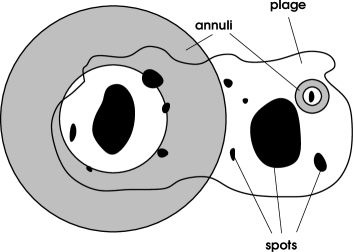
Figure 5: Sketch illustrating the origin of the correlation in Figure 3b. The annulus around small spots lies in the plage in its full extent, so these spots are surrounded by the stronger plage fields.

To resolve this dilemma, we generated artificial data sets with the same values of $A_{0}$ and $B_{\mbox{\scriptsize pl}}$ as the real data, but with $(\log D)^{\prime}$ values generated artificially by the formula

$$(\log D)^{\prime}=a_{1}-a_{2}B_{\mbox{\scriptsize pl}}+a_{3}x$$ (8)

where $x$ is a random variable of zero mean with a $\sigma=1$ Gaussian probability density. In order to test our null hypothesis we first set $a_{2}=0$, i.e. assume that no real physical correlation exists between $(\log D)^{\prime}$ and $B_{\mbox{\scriptsize pl}}$. Then we submit our data set to a selection designed to mimic the observational bias affecting the real data. More specifically, we take the expected number of data for a given spot equal to its lifetime (as observations are normally made daily), which is in turn calculated assuming that $(\log D)^{\prime}$ stays constant during the decay of the spot.

The parameters $a_{1}$ and $a_{3}$ are freely adjustable, but subject to the condition that the resulting range of “observed” $(\log D)^{\prime}$ values should coincide with the real range. After having computed a large number of simultaneous distributions with a wide variety of $a_{1}$ and $a_{3}$ values we had to conclude that no parameter combination is able to yield a correlation coefficient higher than about $0.1$ in typical realizations. The optimal agreement was found in the case $a_{1}=a_{2}=0$, $a_{3}=0.3$, shown in Figure 4d. It is apparent that the correlation coefficient does not differ from zero by more than $1\sigma$. It seems therefore that the indirect effect of the correlations shown in panels $b$ and $c$ is insufficient to fully explain the correlation found in panel $a$, part of which must be a real physical effect. Indeed, if in our simulated data we allow $a_{2}\neq 0$ it becomes straightforward to find a good representation of the data: $a_{1}=0$, $a_{2}=0.3$, $a_{3}=0.4$ is for instance just such a case (not shown here).

We thus conclude that while selection effects probably contribute to the anticorrelation of $(\log D)^{\prime}$ with the plage field strength around spots, a part of this effect is likely to have a physical origin.

5 Theoretical interpretation

In order to understand the origin of a physical anticorrelation between $(\log D)^{\prime}$ and the value of the external magnetic field strength here we extend the turbulent erosion model of sunspot decay for the case when the flux tube is embedded in a preexisting parallel homogeneous magnetic field. Apart from this generalization, we consider the same cylindrically symmetric case as in PM97, i.e. we solve the nonlinear diffusion equation

$$\frac{\partial}{\partial t}\left(\tilde{r}B\right)=\frac{\partial}{\partial\tilde{r}}\left[\tilde{r}\;\nu(B)\;\frac{\partial B}{\partial\tilde{r}}\right]$$ (9)

where $B$ is the magnetic flux density, $\tilde{r}$ is the radial coordinate, and $\nu$ is the turbulent magnetic diffusivity. For the dependence of the diffusivity on the magnetic field we still consider the same function satisfying the basic physical requirements:

$$\nu(B)=\frac{\nu_{0}}{1+|B/B_{\mbox{\scriptsize e}}|^{\alpha_{\nu}}}.$$ (10)

Here $\nu_{0}$ is the unperturbed value of the diffusivity, and $\alpha_{\nu}$ is a parameter quantifying the steepness of the diffusivity cutoff near $B_{\mbox{\scriptsize e}}$, the latter being the field strength where the diffusivity is reduced by 50 %. Physically, one expects $B_{\mbox{\scriptsize e}}\sim B_{\mbox{\scriptsize eq}}$, the kinetic energy density of photospheric turbulence.

Using the notation $b\equiv B/B_{\mbox{\scriptsize e}}$, our initial conditions will now be

$$b(r)=b_{\infty}+\frac{b_{0}-b_{\infty}}{1+(r/r_{0})^{22}}$$ (11)

where $b_{0}$ is the normalized field strength at the center of the tube, and $b_{\infty}$ is the external (“plage”) field strength: we now assume $b_{\infty}\neq 0$. In this formula $r_{0}$ is the initial radius of the tube at time $t=0$; for a comparison with observations it may be identified with the maximal equivalent radius of the spot.

The values of the current sheet velocity $w$ are plotted against $b_{\infty}$ for different numerical solutions of Equations (9)–(11) in Figure 6. It is apparent that for $b_{\infty}=0$ all the solutions are in agreement with the formula

$$w\simeq C{\nu_{0}}/{r_{0}}(b_{0}-1),$$ (12)

with $C\simeq 1.2$, as expected.

Figure 6: Current sheet velocity $w$ as a function of the background field strength $b_{\infty}$. $\Diamond$: $\alpha_{\nu}=2.3$, $b_{0}=30$; $\Box$: $\alpha_{\nu}=2.5$, $b_{0}=10$; $\triangle$: $\alpha_{\nu}=3.0$, $b_{0}=10$; $\ast$: $\alpha_{\nu}=4.5$, $b_{0}=10$; $+$: $\alpha_{\nu}=7$, $b_{0}=3$. The dashed line is just a fiducial straight line, drawn to aid the eye. Solid line: eq. (B-3)

With intermediate values of $\alpha_{\nu}\sim 2$–$3$ the dependence of $w$ on $b_{\infty}$ is approximately logarithmic for $b_{\infty}\mathrel{\mathchoice{\vbox{\offinterlineskip\halign{\hfil$\displaystyle#$\hfil\cr>\cr\sim\cr}}}{\vbox{\offinterlineskip\halign{\hfil$\textstyle#$\hfil\cr>\cr\sim\cr}}}{\vbox{\offinterlineskip\halign{\hfil$\scriptstyle#$\hfil\cr>\cr\sim\cr}}}{\vbox{\offinterlineskip\halign{\hfil$\scriptscriptstyle#$\hfil\cr>\cr\sim\cr}}}}-1$, while for $\alpha_{\nu}>4$ it is strongly reduced for $b_{\infty}>0$. The high-$\alpha_{\nu}$ behaviour may be interpreted in terms of a generalization of the dimensional argument leading to (12), see Appendix B.

The actual value of $\alpha_{\nu}$ is poorly known, but from Figure 6 it is clear that in the range $-1<b_{\infty}<1$ the rate of flux loss should depend approximately logarithmically on $b_{\infty}$, independently of the value of $\alpha_{\nu}$. In other words, the background field acts as multiplicative noise in the decay process. Setting $B_{\mbox{\scriptsize e}}\simeq B_{\mbox{\scriptsize eq}}\simeq 400$G, the photospheric value, this logarithmic relation is plotted over the observational data in Figure 4a. The apparent good agreement lends further support to the physical reality of the correlation found in the previous section.

6 Conclusion

6.1 Proposition: decay rate deviations as effects of the plage field

The theoretical results presented in Section 5 suggest the following scheme for the origin of random deviations from the mean parabolic decay law (1). It is rather natural to assume that the value of the background plage field strength of independent origin shows a Gaussian probability distribution around some expected value around a spot. Figure 6 then implies that the flux loss rate from the flux tube should be characterized by a lognormal distribution (just as we found in Section 2), and that an anticorrelation should exist between the logarithmic decay rate fluctuations $(\log D)^{\prime}$ and the strength of the plage field surrounding the spots (just as we found in Section 4). The generalization of the erosion model to the case of a tube embedded in an external homogeneous magnetic field then apparently offers a simple and elegant explanation for the presence of large lognormally distributed deviations from the mean decay rate in individual spots.

It should be noted that a relation between the decay rate of sunspots and their environment was also suggested by Antalová and Mačura (1985). While Moreno-Insertis and Vázquez (1988) correctly pointed out that the existence of a bimodal distribution of decay rates (i.e. well-separated branches of fast- and slow-decaying spots in the area–decay rate plane) in that study was the consequence of a trivial selection effect, the apparent physical difference found by Antalová and Mačura (1985) between the two classes (slow-decaying spots tending to be “naked” spots in the sense defined by Liggett and Zirin, 1983) still remains, and it may possibly be related to the environmental effect proposed in the present work.

6.2 Caveats and call for more data

However attractive the scheme outlined in the previous subsection may seem, it is almost certainly an oversimplification of the real situation. Firstly, it is obvious from Figure 4a that a large part of the scatter in $(\log D)^{\prime}$ is independent of $B_{\mbox{\scriptsize pl}}$. Though part of this scatter may be due to our method of deriving the vertical field component by deprojecting the line-of-sight component measured, etc., one may expect that effects like deviations from axial symmetry and sub-photospheric forces should necessarily contribute a great deal to deviations from the relation predicted by the erosional model. It is therefore certainly not the case that the lognormal distribution of decay rates can be explained by the plage effect alone: however, owing to the central value theorem of probability theory, the lognormal distribution can be saved if the other influences also act as multiplicative noise.

Another caveat is related to the strong influence of the bias treated in Section 3.3.2 of Paper I throughout this analysis. Though, as we have seen, it is not impossible to correct for these effects, some fine points and simplifications in the correction process may always leave some doubt concerning the robustness of the conclusions derived. The main difficulties here are all due to the fact that our data (like all solar patrols realized in this outgoing century) were taken on a daily basis. One of the most emphatic conclusions of this study is that observations made on a daily basis are insufficient for an in-depth study of the sunspot decay process. What is needed is at least one observational campaign lasting several months, preferably at the time of solar maximum, with several simultaneous white-light heliogram and magnetogram observations a day. Only from the use of such higher quality data can we expect the final illumination of the sunspot decay problem.

Figure 7: Total spot areas from the DPR 1977 plotted against their difference from the areas calculated by multiplying by 6.2 the corresponding umbral areas of the Mt Wilson catalogue. The size of the symbols is related to the central meridian (CM) distance of the spot, $|L-L_{CM}|$; the scale of symbol sizes is set by three examples given in the top right corner.

In an attempt to extend our database we examined the possibility of incorporating Mt Wilson observations in our data (Howard, Gilman, and Gilman, 1984). One problem to be solved here was that in the Mt Wilson catalogue the spots are not identified from one day to the next, so in order to calculate decay rates the identification had to be done. We developed an algorithm for the identification of spots taking into account the differential rotation. A comparison of the results with the published DPR data, where available, showed that the identification has an acceptable rate of success, at least for the larger spots in each active region (which tend to dominate our data set).

A further difficulty is caused however by the fact that the Mt Wilson data only yield estimated umbral areas. Umbral areas are notoriously more difficult to determine than umbra+penumbra areas (Győri, 1998); besides, the method of determination applied was rather approximate (Howard, Gilman, and Gilman, 1984). While it is possible to translate umbral areas $A_{U}$ into total areas $A$ by the simple linear rule $A=6.2\,A_{U}$ (the value of the coefficient was determined from an analysis of DPR area data), this linear relation involves a large scatter, further contributing to the uncertainty of the area values. The resulting large errors are borne out in Figure 7, where we plotted the difference between the MtWilson area values thus derived and the corresponding DPR area values against DPR areas for 1977. It is apparent that the scatter is very large indeed, effectively excluding the use of Mt Wilson data for our present purpose.

Figure 8: Sketch showing the characteristic shape and scales of the magnetic field profile (solid) and of the stationary solution (B-1) (dashed) near the outer edge of the current sheet. $r_{1}\equiv b/(db/dr)$ at $r=1$

It may be worth noting that Figure 7 also seems to suggest a systematic trend: the areas computed from Mt Wilson data are lower than their DPR counterparts for large spots, while the reverse tends to be the case with small spots. One possible interpretation could be that the fixed ratio $A/A_{U}=6.2$ used here may be incorrect, and that the umbral/total area ratio may in fact have some mean area dependence. However, a similar plot constructed using the DPR umbral areas instead of the Mt Wilson areas does not show any obvious trend (while it still shows a high scatter), which seems to exclude this explanation. The trend mentioned is then probably due to differences in the applied methods of area measurement.

Appendix B: Analytical interpretation of the high-$\alpha_{\nu}$ behaviour of the generalized erosion models

For simplicity we set the units of time and length so that $\nu_{0}=1$ and $b(1)=1$. Restricting our interest to the case $b_{0}\gg 1$, from (12) $w\ll 1$ follows, so that in the range $1<r<1+r_{1}$ the solution may be approximated as the stationary solution of the linear diffusion equation in cylindrical geometry (cf. Fig. 8):

$$b=1-\frac{\ln r}{r_{1}}$$ (B-1)

From the numerical solutions we know that the erosional (i.e. nearly form-invariant propagating) solution forms after an initial transition time $t_{i}\sim 1$. If the initial profile at $t=0$ is sufficiently steep [as is the case with (11)] then at $t=t_{i}$ the amount of magnetic flux outside $r=1$ equals the flux lost from within the CS, and the original plage flux there:

$$2\pi\int_{1}^{1+r_{1}}rb(r)\,dr\simeq\pi b_{0}(r_{0}^{2}-1)+\pi b_{\infty}(r_{1}^{2}+2r_{1})$$ (B-2)

As we are still within about one diffusive timescale from $t=0$, practically all this flux must still lie inside the radius $1+r_{1}$, where the approximation (B-1) may be used for $b(r)$. On the other hand, $r_{0}=1+wt_{i}$, while $w$ and $r_{1}$ are related by $w\simeq[r_{1}(b_{0}-1)]^{-1}$ (PM97, eq. (10)), so, neglecting a term of order $b_{0}^{-2}$, we have

$$(r_{1}^{2}+2r_{1})\left(1+\frac{1}{2r_{1}}-b_{\infty}\right)-\frac{(1+r_{1})^{2}}{r_{1}}\ln(1+r_{1})-\frac{2b_{0}}{b_{0}-1}r_{1}=0$$ (B-3)

Setting $t_{i}=1$ and $b_{0}=10$, Equation (B-3) can be solved numerically for $r_{1}$, and thus for $w\simeq[r_{1}(b_{0}-1)]^{-1}$; the solution turns out to be a very nearly linear function of $b_{\infty}$ (solid curve in Figure 6).

Appl. Opt.
K. Petrovay
Instituto de Astrofísica de Canarias
La Laguna, Tenerife, E-38200 Spain
E-mail: kpetro@iac.es

References

- Antalová and Mačura (1985) Antalová, A. and Mačura, R.: 1985, Contr. Skaln. Pleso Obs. 14, 163
- Dezső, Gerlei, and Kovács (1987) Dezső, L., Gerlei, O., and Kovács, Á.: 1987, Debrecen Photoheliographic Results for the year 1977, Publ. Debrecen Heliophys. Obs., Heliogr. Series No. 1, Debrecen
- Dezső, Gerlei, and Kovács (1996) Dezső, L., Gerlei, O., and Kovács, Á.: 1996, Debrecen Photoheliographic Results for the year 1978, Publ. Debrecen Heliophys. Obs., Heliogr. Series No. 2, ftp://fenyi.sci.klte.hu/pub/DPR/1978
- Győri (1998) Győri, L.: 1998, Solar Phys. 180, 109
- Howard (1992) Howard, R.: 1992, Solar Phys. 137, 51
- Howard, Gilman, and Gilman (1984) Howard, R., Gilman, P. A., and Gilman, P. I.: 1984, Astrophys. J. 283, 373
- Liggett and Zirin (1983) Liggett, M. and Zirin, H.: 1983, Solar Phys. 84, 3
- Martínez Pillet, Moreno-Insertis, and Vázquez (1993) Martínez Pillet, V., Moreno-Insertis, F., and Vázquez, M.: 1993, Astron. Astrophys. 274, 521 (MMV93)
- Moreno-Insertis and Vázquez (1988) Moreno-Insertis, F. and Vázquez, M.: 1988, Astron. Astrophys. 205, 289
- Oakley et al. (1994) Oakley, D. S., Snodgrass, H. B., Ulrich, R. K., and VanDeKop, T. L.: 1994, Astrophys. J. 437, L63
- Petrovay (1998) Petrovay, K.: 1998, A crossroads for european solar and heliospheric physics: recent achievements and future mission possibilities, ESA Publ. SP-417, p. 273
- Petrovay and Moreno-Insertis (1997) Petrovay, K. and Moreno-Insertis, F.: 1997, Astrophys. J. 485, 398 (PM97)
- Petrovay and van Driel-Gesztelyi (1997) Petrovay, K. and van Driel-Gesztelyi, L.: 1997, Solar Phys. 176, 249 (Paper I)
- Walther (1998) Walther, G.: 1998, Astrophys. J. 513, 990