Determining the Physical Properties of the B Stars I. Methodology and First Results

Abstract

We describe a new approach to fitting the UV-to-optical spectra of B stars to model atmospheres and present initial results. Using a sample of lightly reddened stars, we demonstrate that the Kurucz model atmospheres can produce excellent fits to either combined low dispersion IUE and optical photometry or HST FOS spectrophotometry, as long as the following conditions are fulfilled:

1. an extended grid of Kurucz models is employed,

2. the IUE NEWSIPS data are placed on the FOS absolute flux system using the Massa & Fitzpatrick (1999) transformation, and

3. all of the model parameters and the effects of interstellar extinction are solved for simultaneously.

When these steps are taken, the temperatures, gravities, abundances and microturbulence velocities of lightly reddened B0-A0 V stars are determined to high precision. We also demonstrate that the same procedure can be used to fit the energy distributions of stars which are reddened by any UV extinction curve which can be expressed by the Fitzpatrick & Massa (1990) parameterization scheme.

We present an initial set of results and verify our approach through comparisons with angular diameter measurements and the parameters derived for an eclipsing B star binary. We demonstrate that the metallicity derived from the ATLAS 9 fits to main sequence B stars is essentially the Fe abundance. We find that a near zero microturbulence velocity provides the best-fit to all but the hottest or most luminous stars (where it may become a surrogate for atmospheric expansion), and that the use of white dwarfs to calibrate UV spectrophotometry is valid.

1. Introduction

The goal of modeling the observed spectral energy distribution (SED) of a star is straightforward, namely, to obtain information on the physical properties of a star from the model atmosphere which fits the observations best. After the best-fitting model is found, it is assumed that the parameters which define the model (effective temperature, surface gravity, elemental abundances, etc.) faithfully represent those of the star itself. The degree to which this key assumption is valid depends upon both the uniqueness of the fit (requiring a firm understanding of all observational errors) and the appropriateness of the physical assumptions used to construct the models (which often can be verified by ancillary information). If the fit provides strong constraints on the model parameters and the model is considered valid, then this “continuum fitting” process provides a powerful tool for studying stellar properties.

There are two major motivations for modeling the UV/optical SED’s of the main sequence B stars. First, since 70-to-100% of the energy of B stars (with 10000 $<T_{eff}<$30000 K) is emitted in the accessible spectral region between 1216 Å and 1 $\mu$m (see Fig. 1 of Bless & Percival 1997), even low-resolution UV/optical observations can place strong constraints on stellar models and should provide robust determinations of the stellar properties which influence the SED (particularly $T_{eff}$ and the surface gravity $\log g$). Second, the shape of the B star SED’s in the UV is also influenced by opacity due to Fe group elements (Cr, Mn, Fe, Co, Ni), and thus should allow constraints to be placed on Fe group abundances — without the modeling of individual line profiles. Such results, particularly if attainable with low-resolution data, would be extremely useful for studying stellar metallicity patterns when combined with ground-based determinations of CNO abundances (e.g., Smartt & Rolleston 1997, Dufton 1998, Gummersbach et al. 1998) since only the coolest of the B stars have sufficient lines in their optical spectra to allow accurate Fe group abundances to be derived from the ground.

Accessing the information content of the B star UV/optical SED’s requires a set of model atmospheres which reproduce the physical structure and emergent flux of the B star atmospheres. The main sequence B stars are the hottest, most massive, and most luminous stars whose atmospheric structures are believed to be well-represented by the simplifying assumptions of local thermodynamic equilibrium (LTE), plane parallel geometry, and hydrostatic equilibrium. Thus, although it is clear that a full non-LTE analysis may be needed for detailed modeling of specific line profiles, LTE model atmosphere calculations are expected to reproduce the atmospheric structures and gross emergent flux distributions of these stars (e.g., Anderson 1985, 1989; Anderson & Grigsby 1991; Grigsby, Morrison, & Anderson 1992; Gummersbach et al. 1998). As a result, the line-blanketed model atmospheres computed by R.L. Kurucz, which incorporate the simplifying assumptions listed above, have become a standard tool in the study of B stars. These ATLAS-series models have been used in a wide variety of investigations, including the determination of fundamental stellar parameters (e.g., Code et al. 1976); population synthesis (e.g., Leitherer et al. 1996); stellar abundances within the Galaxy (e.g., Geis & Lambert 1992; Cuhna & Lambert 1994; Smartt & Rolleston 1997; Gummersbach et al. 1998) and among the nearby Galaxies (e.g., Rolleston et al. 1996 and references therein); the physical structure of atmospheres of the pulsating $\beta$ Cephei stars (e.g., Cugier et al. 1996); the derivation of interstellar extinction curves (e.g., Aannestad 1995); the determinations of the distances to binary Cepheids (e.g., Böhm-Vitense 1985); and many others.

Despite the long history of “continuum fitting” the UV/optical SED’s of B stars (see, e.g., Code et al. 1976, Underhill et al. 1979; Remie & Lamers 1982; and Malagnini, Faraggiana, & Morossi 1983; among many others), several key issues regarding the applicability of the ATLAS models to the B stars have not yet been addressed quantitatively. These include the range of stellar properties over which the physical assumptions and simplifications are valid (or, at least, not debilitating) and whether — within that range — the models truly reproduce the observations. Most previous applications of the continuum fitting technique have relied on “by eye” fitting, have attempted to deduce only $T_{eff}$, and have utilized crude treatments of interstellar extinction. Thus it is not clear whether the often large discrepancies seen in the UV region, in particular, are attributable to failures in the models or to shortcomings in the fitting process.

Because of their ubiquity, great diagnostic potential, and relative ease of calculation, the ATLAS models are a tremendous resource for stellar astronomy and a quantitative assessment of their range of applicability is imperative. Recent significant advances in the requisite theoretical and observational material make this an ideal time to undertake such an investigation. These advances include the release of the ATLAS 9 models with their greatly improved opacities (Kurucz 1991), the re-processing of the entire International Ultraviolet Explorer (IUE) low-resolution UV spectrophotometry archives, the derivation of a precise UV calibration by the HST Faint Object Spectrograph (FOS) team (Bohlin 1996, and see Bless & Percival 1997), the derivation of a rigorous transformation between the IUE and FOS calibration systems (Massa & Fitzpatrick 1999, hereafter MF99), and an improved understanding of the properties of UV/optical interstellar extinction (Fitzpatrick & Massa 1990, hereafter FM; Fitzpatrick 1999, hereafter F99).

This paper is the first in a series whose goals are to quantify the degree of agreement between the ATLAS model atmospheres and UV/optical spectrophotometry of B stars and to apply the models to determine the physical properties of the stars and the wavelength dependence of interstellar extinction. Here we discuss the methodology to be employed by our study and present some initial results. In §2, we provide an overview of modeling observed energy distributions and describe the essential ingredients of the fits: a complete set of model atmosphere calculations, and a quantitative characterization of the effects of interstellar extinction. The section concludes with a description of the mathematical procedure used to fit the models to the observations and a brief discussion of the determination of metallicity using the ATLAS 9 models. In §3, we describe the spectrophotometric observations we will be modeling and §4 provides a sample of our results, illustrating the quality of the fits, the agreement between the derived parameters and fundamental measurements, and a comparison with previous, independent abundance measurements. The potential for future study is also discussed. Finally, §5 summarizes our findings and outline a few remaining technical issues.

2. Modeling the Observed Stellar Fluxes

In this section, we provide an overview of the general problem of fitting stellar energy distributions, describe the constituents of the model used to fit the observations, and discuss how the fitting is accomplished.

2.1. Overview of the problem

The energy distribution of a star as received at the earth, $f_{\lambda\oplus}$, depends on the surface flux of the star and on the attenuating effects of distance and interstellar extinction. This observed flux at wavelength $\lambda$ can be expressed as:

$$f_{\lambda\oplus} = F(\{\alpha\})_{\lambda}\times\left(\frac{R}{d}\right)^{2}\times 10^{-0.4A(\lambda)}$$ (1)

$$= F(\{\alpha\})_{\lambda}\times\left(\frac{R}{d}\right)^{2}\times 10^{-0.4E(B-V)[k(\lambda-V)+R(V)]}$$ (2)

where $F_{\lambda}$ is the emergent flux at the surface of the star (assumed to be single), $\{\alpha\}$ is the set of intrinsic physical properties which determine the emergent flux from the star, $R$ is the stellar radius, $d$ is the distance to the star and $A(\lambda)$ is the total extinction along the line of sight. The factor $(R/d)^{2}$ is essentially equivalent to the square of the angular radius of the star and is often written as ($\theta/2)^{2}$, where $\theta$ is the stellar angular diameter.

In eq. 2, the extinction terms are rewritten as quantities normalized by $E(B-V)$, i.e., the normalized extinction curve $k(\lambda-V)=[A(\lambda)-A(V)]/E(B-V)$, and the ratio of selective to total extinction in the $V$ band $R(V)\equiv A(V)/E(B-V)$.

2.2. The models

We represent the stellar surface fluxes with R.L. Kurucz’s ATLAS 9 line-blanketed, LTE, plane-parallel, hydrostatic model atmospheres. These models are functions of the 4 parameters $\{\alpha\}$ = $\{T_{eff},\log g,{\rm[m/H]},v_{t}\}$ – which are the effective temperature, the log of the surface gravity, the logarithmic metal abundance relative to the Sun, and the magnitude of the microturbulent velocity field, respectively. The standard ATLAS 9 calculations provide emergent fluxes at 1221 square-binned wavelength points from 90.9 Å to 160 $\mu$. The bin widths are typically 10 Å in the UV (300 Å $<\lambda<$ 3000 Å) and 20 Å in the optical (3000 Å$<\lambda<$ 10000 Å).

Because the fitting procedure must be given access to the entire region of parameter space which is physically reasonable, it was necessary extend the standard Kurucz grid, which contains only $v_{t}=2$ km s^-1 models. This was accomplished using the ATLAS 9 programs and input Opacity Distribution Functions (ODFs) to compute additional model atmospheres and emergent fluxes. We expanded the grid to include $v_{t}=0,4,8$ km s^-1, [m/H] $=-1.5$, $-1.0$, $-0.5$, 0.0, +0.5 (i.e., from 1/30 to 3$\times$ solar), 36 values of $T_{eff}$ between 9000 and 50000 K, and typically $\sim 10$ values of $\log g$ for each $T_{eff}$ extending from the Eddington limit to $\log g=5.0$. Our final grid consists of emergent flux distributions for about 7000 models.

In order to calculate a model at a set of parameters $\{T_{eff}^{*},\log g^{*},{\rm[m/H]}^{*},v_{t}^{*}\}$ which do not exactly coincide with a grid point, an interpolation scheme in all 4 parameters is required. We adopt the following approach: First, at the three grid values of $v_{t}$ closest to $v_{t}^{*}$ and the three grid values closest to [m/H]^∗, we produce models with $T_{eff}^{*}$ and $\log g^{*}$ through bilinear interpolation of $\log F_{\lambda}$ against $\log T_{eff}$ and $\log g$. This yields 9 models. Next, we quadratically interpolate $\log F_{\lambda}$ against [m/H] at each of the $v_{t}$, producing 3 models of the desired $T_{eff}^{*}$, $\log g^{*}$, and [m/H]^∗. Finally, we quadratically interpolate $\log F_{\lambda}$ against $v_{t}$ to obtain the final model. Tests of this procedure against models computed “from scratch” at $\{T_{eff}^{*},\log g^{*},{\rm[m/H]}^{*},v_{t}^{*}\}$ indicate that the errors introduced are negligible.

In addition to fluxes, we produced synthetic Johnson $UBV$ and Strömgren $uvby$ photometry for each model, using the programs of Buser & Kurucz (1978) and Relyea & Kurucz (1978). The value of the synthetic V magnitude $V_{syn}$ — which is used in the current fitting procedure — is determined by the following:

$$V_{syn}=-21.07-2.5\times\log\int{f_{\lambda}S_{\lambda}(V)d\lambda}$$ (3)

where $f_{\lambda}$ is a stellar SED (either observed or theoretical) and $S_{\lambda}(V)$ is the normalized filter sensitivity function for the $V$ filter from Azusienis & Straizys (1969). The integration is performed over the $V$ filter’s range of response (4750 Å to 7400 Å). The normalization zeropoint, $-21.07$, was determined from synthetic photometry performed on FOS spectrophotometry of seven calibration stars (Colina & Bohlin 1994; Bohlin, Colina, & Finley 1995) and on ground-based spectrophotometry of HD 172167 (Vega; Hayes 1985). For these eight stars, equation 3 yields a standard deviation of 0.01 mag in the difference $V-V_{syn}$, consistent with expected observational error.

2.3. Interstellar extinction

Correcting stellar SED’s for the effects of interstellar extinction is problematical because the wavelength dependence of extinction is known to be highly variable spatially. While average extinction curves have been defined, there may be few if any sightlines for which some globally-defined mean curve is strictly appropriate. Furthermore, the error introduced by using an inappropriate curve increases in proportion to the amount of extinction (see Massa 1987). Consequently, we adopt one of two approaches for modeling extinction, depending on the color excess of the object. For lightly reddened stars ($E(B-V)<0.1$) we adopt a universal mean curve and solve only for $E(B-V)$. For the more reddened stars, we investigate the feasibility of deriving both $E(B-V)$ and the shape of the extinction curve from the data themselves. In both cases we utilize an analytical representation for the extinction wavelength dependence based on the work of FM.

For the universal mean curve, we use the results of F99. These are based on the general UV curve parameterization of FM and the discovery by Cardelli et al. (1989) that the shape of UV extinction curves correlate with the extinction parameter $R(V)$, defined in §2.1. F99 presents a mean curve for the case of $R(V)=3.1$ which (when applied to a stellar energy distribution and convolved with the appropriate filter responses) reproduces the mean extinction ratios found in the optical and IR from the Johnson and Strömgren photometric systems. The curve also joins smoothly with the UV region (at $\lambda\leq 2700$Å) via cubic spline interpolation. The UV portion of the curve is expressed as a set of three smooth functions and specified by 6 parameters, all adjusted to their nominal values for the case $R(V)=3.1$.

For the more heavily reddened stars, we allow for additional free parameters (i.e, in addition to $E(B-V)$) so that a “customized” extinction curve can be derived by solving for some or all of a modified version of the FM curve parameters. FM showed that any normalized UV extinction curve can be represented by 6 parameters which describe the general slope and curvature of the curve and the position, width, and strength of the 2175 Å bump. We modify this approach slightly, in that the linear terms are combined (FM show that these are functionally related) and we use a cubic spline to bridge the gap between the UV at 2700 Å and the normalized optical curve near 4100 Å (see F99). Consequently, the most general UV/optical extinction curve contains 5 free parameters. The feasibility of this approach is demonstrated in §4.

2.4. Fitting the spectra – qualitative considerations

The ability to extract the physical parameters of a model accurately from the observed SED depends on whether changes in those parameters produce detectable and unique spectral signatures. In Figure 1, we illustrate the signatures of the five principal parameters considered in the fitting process for a typical B star model flux distribution. The top panel shows the UV/blue-optical SED for an ATLAS 9 model with parameters as listed in the figure. The five lower panels show the effects on the spectrum caused by changes in the physical parameters $\{\Delta T_{eff},\Delta\log g,\Delta{\rm[m/H]},\Delta v_{t}\}=\{+100{\rm K},+0.1{\rm dex},+0.1,{\rm dex},+1{\rm kms}^{-1}\}$ and by a change $\Delta E(B-V)=$ +0.005 mag in the amount of interstellar extinction present.

Three aspects of the figure are important:

1. The spectral signatures of the four stellar parameters are functionally independent, i.e., it is not possible to construct any one effect from a linear combination of the others. Consequently, it should be possible to derive unambiguous and uncorrelated estimates for each of the parameters from the data.

2. The signature of interstellar extinction is quite distinct from those of the model parameters and, in principal, the value of $E(B-V)$ should be precisely determined by the fitting procedure.

3. The RMS magnitudes of each of the effects in the UV region are of order 0.01 dex. Since we will be fitting more than 100 data points in the UV with typical RMS errors of 3% per point, uncertainties in the physical parameters corresponding to the differences shown in the figure should be well within our grasp.

Note that the strength and shape of each of the spectral signatures shown in Figure 1 — and their degree of independence from each other — do vary as a function of the model parameters, particularly $T_{eff}$. Therefore, the precision achievable in estimating the parameters will differ across the wide range of $T_{eff}$ values appropriate for the B stars.

It might seem surprising that $v_{t}$ and [m/H] can each be determined independently of the other, since both directly affect the absorption lines. This can be understood in principle, however, from considering the curve-of-growth, which describes the strength of an absorption feature as a function of the various relevant physical properties of a system. In particular, variations in the number of available absorbers (e.g., [m/H]) mainly affect weak, unsaturated absorption lines on the “linear part” of the curve-of-growth, while variations in line broadening (e.g., $v_{t}$) mainly affect the stronger, saturated lines on the “flat part” of the curve-of-growth. Thus, changes in [m/H] and $v_{t}$ have their greatest effects on distinct populations of lines (although there is a large “middle ground” in which both parameters are important). This can be seen in Figure 1 where the spectral features near 2000 Å respond dramatically to a change in $v_{t}$ and much less so to a change in [m/H]. The inverse can be seen for features in the 1300–1500 Å region.

The ability to distinguish microturbulence effects from abundance effects appears to breakdown for cases where $v_{t}$ is large. In §4 we show several stars for which the combination of a high microturbulence and a low metallicity reproduce the observed UV opacity very well — although their individual values are unlikely to represent the corresponding stellar properties. As discussed in §4, this probably indicates that microturbulence is a physically incorrect description of the line broadening mechanism in these stars.

2.5. Fitting the spectra – quantitative considerations

In practice, we fit equation (2) recast into the following form

$$\log f_{\lambda\oplus} = \log\left[\left(\frac{R}{d}\right)^{2}\times 10^{-0.4A(V)}\right]$$ (4)

$$+\log F(T_{eff},\log g,[\rm m/H],\it v_{t})_{\lambda}$$

$$-0.4E(B-V)k(\lambda-V)$$

We refer to the leading term as the “attenuation factor” because it is independent of wavelength. It contains the distance, stellar size and total extinction information. The second term is the stellar model which has a non-linear wavelength dependence on the 4 model parameters. The final term expresses the magnitude and wavelength dependence of interstellar extinction and it can represented as either a simple linear function (in the case of predefined extinction curve) or a more complex function involving both linear and non-linear terms (see §2.3). In general, there can be anywhere between 6 and 11 free parameters, depending on how much flexibility is incorporated into the description of reddening.

Notice that, since we do not utilize infrared photometry in our program, we cannot determine the value of $R(V)$ from the fitting procedure. Instead, we adopt a typical value (usually $R(V)=3.1$) and then incorporate the expected uncertainty into the error estimate of $\log(R/d)^{2}$ (an uncertainty in $R(V)$ does not affect the stellar parameters or $k(\lambda-V)$).

The best-fitting model is obtained by solving equation (4) for all of the unknown parameters simultaneously. We use an iterative, weighted non-linear least squares technique (the Marquardt method) to adjust the parameters and minimize the $\chi^{2}$ of the fit. The parameter values used to initialize the fitting procedure are determined from the spectral type and optical photometry of the star. The only constraint we impose on the domain of the model parameters is that $v_{t}$ and $E(B-V)$ be $\geq 0$. Note that $E(B-V)$ is simply a scaling factor for $k(\lambda-V)$, and we do not utilize $(B-V)$ photometry in the fits at this time.

The degree of accuracy to which any single parameter can be determined depends on the sensitivity of the observed flux to that parameter and on the degree of covariance with the other parameters (e.g., see Fig. 1). Our error analysis incorporates the full interdependence of the various parameters and includes the effects of random noise in the data. All uncertainties quoted in this paper are 1-$\sigma$ internal fitting errors, in the sense that a change in a particular parameter by $\pm$1-$\sigma$ results in a change in the total $\chi^{2}$ by +1 after all the other parameters have been reoptimized (see Bevington 1969, Chapter 11).

2.6. Abundances from ATLAS 9 models

The definition and impact of the metallicity, [m/H], in the ATLAS 9 models requires special attention. Different metallicities are achieved by scaling the abundances of all elements heavier than He by a single factor relative to the reference solar photosphere abundances ([m/H$]=0$) given by Grevesse & Anders (1989). Clearly, a single parameter is insufficient to describe the results of the complex physical processes which control the variations in stellar abundance patterns. Nevertheless, it is equally clear that such a parameter can provide a useful diagnostic if it can be determined robustly and with high precision from relatively low resolution data.

The UV spectral region of all main sequence B stars ($10,000<T_{eff}<30,000$ K) is extremely rich in Fe group lines (e.g., Walborn et al. 1995, Roundtree & Sonneborn 1993), which are obvious even at low resolution (Swings et al. 1973). The sensitivity of the ATLAS 9 models to changes in [m/H] is dominated by changes in Fe (except over narrow intervals where the presence of a few strong, isolated silicon and carbon lines becomes important, see Massa 1989). This assertion is justified in Figure 2 where the solid curves show how of a $-0.1$ dex change in [m/H] affects the UV SED’s for three values of $T_{eff}$ which span the range of the B stars. Below each curve, the shaded regions show the sum of the $gf$ values (arbitrarily scaled and shifted) for the all spectral lines of Fe IV (top panel), Fe III (middle panel), and Fe II (bottom panel) within each ATLAS 9 wavelength bin. Thus, the shaded regions crudely illustrate the relative strength and general wavelength distribution of the Fe opacity in the UV. In the figure, the $\Delta\log F_{\lambda}$ curves have been paired with Fe ions likely to be dominant, although absorption due to adjacent ionization stages will also be present.

In each of the panels the opacity signature of the various Fe ions is strikingly similar to the signature of $\Delta$[m/H]. It is clear that the value of [m/H] determined by fitting observed SED’s with ATLAS 9 models is most heavily influenced by the abundance of Fe. Therefore we assume that the value of [m/H] derived from large scale UV absorption features in B stars is effectively a measurement of [Fe/H].

Several comments regarding the robustness of an [Fe/H] measurement from fitting the UV SED’s of the B stars can be made:

1. In addition to Fe itself, the other Fe-group elements (Cr, Mn, Fe, Co, Ni) also contribute to the UV opacity, albeit at a much reduced level. However, since all of these elements are thought to have similar nucleosynthetic origins, their abundances are expected (and observed) to scale together naturally. Therefore the ATLAS 9 method of scaling all abundances by a single parameter is physically reasonable for the Fe-group elements and does not confuse the relationship between [m/H] and [Fe/H].

2. The abundances of CNO and the light metals (e.g., Si) certainly have been observed to vary relative to Fe. Fortunately, however, the atmospheric opacity of main sequence B stars is primarily due to hydrogen, helium and Fe. Consequently, even if an ATLAS 9 abundance mix results in too much or too little of CNO or the light metals relative to the Fe group, the impact on the atmospheric structure and, hence, the shape of the low resolution energy distribution is both minimal and localized in wavelength (see the discussion of Vega in §4)

3. The low resolution UV spectral signature of Fe results from the combined opacity of literally thousands of lines. Therefore, random uncertainties in individual f-values or line centers tend to cancel out, as do non-LTE effects in specific lines.

Thus, while the study of element-to-element abundance variations generally requires high resolution stellar data and the computation of synthetic spectra, Fe abundances in main sequence B stars can be determined readily from the gross structure of their low resolution UV spectra.

A second aspect of the ATLAS 9 abundances requires some clarification. The models use a reference solar Fe abundance which is 0.12 dex larger than the currently accepted value (see, e.g., Grevesse & Noels 1993). Since, as demonstrated above, Fe dominates the UV opacity signature from which [m/H] is determined, we adopt the following transformation:

$$\left[\frac{\rm Fe}{\rm H}\right]\simeq\left[\frac{\rm m}{\rm H}\right]+0.12\\$$ (5)

where [m/H] is the metallicity parameter of the best-fitting ATLAS 9 model and [Fe/H] is the actual logarithmic abundance of Fe relative to the true solar value.

A final comment concerns the $\Delta$[m/H] signature at the cool end of the B star range. The lower panel in Figure 2 (for $T_{eff}=10000$ K) shows that, while the mid-UV correlation between $\Delta\log F_{\lambda}$ and the Fe II opacity is unmistakable, the far-UV sensitivity to $\Delta$[m/H] is larger than might readily be explained by Fe alone. Part of this apparent discrepancy is due to changes in the atmospheric temperature structure which result from changing levels of opacity. The far-UV region in these relatively cool models is extremely sensitive to these changes. Thus, some of the rapid rise in $\Delta\log F_{\lambda}$ at short wavelengths is essentially a second order effect of changing the Fe opacity. The presence of strong opacity sources due to elements other than the Fe group also helps produce the far-UV sensitivity to [m/H]. Numerous lines of C I are present at wavelengths shortward of $\sim$1500 Å, along with strong lines of C II, Si II, and other species. When this spectral region is included in the fitting process, the best-fit [m/H] value will represent a compromise between the abundances of Fe and of these lighter elements. For the late B stars, an inability to achieve good fits between observed and theoretical SED’s across the entire UV spectral region might serve to indicate a more complex abundance anomaly than can be represented by a single scale factor. In §4 we will demonstrate this effect in the spectrum of Vega.

3. The Data

The primary data used in our analysis are NEWSIPS low-dispersion IUE UV spectra (Boggess et al. 1978a, 1978b; Nichols & Linsky 1996), corrected and placed on the HST - FOS system (Bohlin 1996) using the algorithms developed by MF99. Data from both the long wavelength (LWR and LWP) and short wavelength (SWP) cameras are required and the wavelength regions covered are 1978–3000 Å and 1150–1978 Å, respectively. For a few stars, UV-through-optical spectrophotometry from the FOS is available. These data typically extend from 1150 Å into the optical spectral region.

The UV/optical spectrophotometry (whether from IUE or FOS) are resampled to match the wavelength binning of the ATLAS 9 model atmosphere calculations in the wavelength regions of interest. Since the resolution of the IUE ($\sim$ 4.5 – 8 Å) is only slightly smaller than the size of the ATLAS 9 UV bins (10 Å), the characteristics of binned IUE data do not exactly match those of ATLAS 9, which may be thought of as resulting from the binning of very high resolution data. In essence, adjacent IUE bins are not independent of each other, while adjacent ATLAS 9 wavelength points are independent. To better match the IUE and ATLAS 9 data, we smooth the ATLAS 9 model fluxes in the IUE wavelength region by a Gaussian function with a FWHM of 6 Å. This slight smoothing simulates the effects of binning lower resolution data. No such smoothing is required when FOS data are used, since they have a much higher resolution than the IUE spectra.

For FOS data, the weight assigned to each wavelength bin is derived from the statistical errors of the data in the bin. The weights for the IUE data are computed likewise, except that an additional, systematic, uncertainty of 3% is quadratically summed with the statistical errors in each bin to account for residual low-frequency uncertainties not removed by the MF99 algorithms.

We give zero weight to the wavelength region 1195 – 1235 Å due to the presence of interstellar Ly $\alpha$ absorption. Additional points may be excluded in particular cases based on data quality or the presense of strong interstellar absorption lines (e.g., Fe II $\lambda\lambda$2344, 2383, 2600, Mg II $\lambda\lambda$2796, 2802) or stellar wind features (e.g., Si IV $\lambda$1400, C IV $\lambda$1550). Apparently spurious model features are present at 2055, 2325, and 2495 Å. These appear as isolated absorption dips in the models, but correspond to no observed stellar lines. Their strengths are temperature dependent, with the 2055 and 2495 Å features present at model temperatures above $\sim$30000 K and the 2325 Å feature strongest at model temperatures below 25000 K (this feature is visible clearly in Figure 1, which also illustrates the metallicity dependence). We routinely give zero weight to these three wavelength bins.

At present, we fit the satellite data and $V$ magnitude data. Eventually, we will expand this to include Johnson $UBV$ and Strömgren $uvby$ photometry, once the calibration of the synthetic photometry is more secure (see §5). Our sources for the Johnson and Strömgren data are the catalogs of Mermilliod (1987) and Hauck & Mermilliod (1990), respectively, when available.

4. Results and discussion

In this section, we demonstrate our fitting process with several examples and discuss the consequences of each. The program stars are listed in Table 1. These stars were selected for three reasons. First, as a group, their physical parameters span the full range of the main sequence B stars. Second, fundamental measurements exist for some of them, and these can be used to verify the accuracy of our results. Third, some of the stars have been the subject of fine analyses, so we can compare our derived stellar parameters to previous estimates, obtained by independent methods.

BD+33^∘ 2642   This is a high latitude post-AGB star and the exciting object of a planetary nebula. Its spectrum was examined in detail by Napiwotzki, Heber, & Köppen (1994; hereafter NHK) who found $T_{eff}=20200$ K, $\log g=2.9$, and a peculiar chemical composition where C, N, O, Mg, and Si are subsolar by about 1 dex and Fe is subsolar by about 2 dex. This star is not typical of the type of object at which our research is aimed; however, it allows us to test the models in two respects. First, it is an extreme case of low metallicity. Second, the FOS data are of exceptional quality, allowing a critical assessment of how well the models can fit the details of an actual stellar energy distribution.

We fit the FOS data for BD+33^∘ 2642 using the $R(V)=3.1$ extinction curve from F99 and we solved for the 4 ATLAS 9 model parameters, $E(B-V)$, and the attenuation factor. The result is presented in Figure 3 where we show the reddening-corrected stellar SED (small filled circles) overplotted with the best-fitting ATLAS 9 model (solid histogram-style curve). The fit is so good that the model and data are nearly indistinguishable over most of the fitted wavelength range, with typical discrepancies less than 2% (consistent with the expected observational errors) except in the regions indicated by crosses. These consist of the excluded ATLAS 9 bins discussed in §3 above and the regions containing the H$\alpha$ and H$\beta$ lines, which show evidence for emission in the FOS data. The model parameters are listed in columns 2–8 of Table 2 along with their 1$\sigma$ internal fitting errors. The attenuation factor is represented by the computed angular diameter of the star $\theta$ (in column 8, in units of milli-arcseconds), as noted in §2.1.

Our temperature for BD+33^∘ 2642 is some 2000 K lower than that found by NHK. This is due entirely to the fact that NHK imposed a value of $E(B-V)=0.06$, while our self-consistent value is significantly smaller ($<0.02$). (The overcorrection for extinction in the 2200 Å region that results from assuming $E(B-V)=0.06$ is apparent in Fig. 3 of NHK). The other parameters derived by NHK will be adversely affected by the overestimated temperature, but are nonetheless generally in reasonable agreement with our results. Our value of [Fe/H$]=-1.5$ is consistent with the NHK Fe abundance ([Fe/H$]=-2.0\pm 0.5$ from IUE data), but suggests that Fe may be more similar in abundance to the other elements than emphasized by NHK. We find a much lower value of $v_{t}$ than NHK, who adopted $v_{t}=15$ km s^-1 based on line profile analysis. Such a large value is inconsistent with the observed UV opacity and might be an artifact of their high $T_{eff}$. It would be interesting to repeat the NHK analysis using the lower temperature given in Table 2.

HV 2274 in the LMC   HV 2274 is a non-interacting eclipsing binary system in the Large Magellanic Cloud which consists of two nearly identical early B stars. The properties of this system and its usefulness as a distance indicator for the LMC are discussed by Guinan et al. (1998). The FOS energy distribution of HV 2274 (ranging from 1150 to 4800 Å) was modeled using the program described here and the results can be seen in Figure 2 of Guinan et al. The fitting was performed by solving for the four model parameters, $E(B-V)$, the attenuation factor, and the six additional parameters from FM which specify the shape of the UV extinction curve. The quality of the fit is comparable to that for BD+33^∘ 2642 discussed above. The significance of HV 2274 for our purposes here is that the surface gravities of the stars in the system are extremely well determined from the properties of the light and radial velocity curves of the binary. This affords the opportunity to test whether the values derived by our approach are reasonable. This is a critical test since it is not necessarily true that good fits to energy distributions produce the correct values of the stellar properties (e.g., see the discussion of HD 38666 and HD 36512 below). The surface gravity of star A of the binary system is known to be $\log g=3.54\pm 0.03$. When the fitting performed with gravity as a free parameter, a completely consistent value of $\log g=3.48\pm 0.06$ was determined. This result gives confidence in the values of the parameters and suggests that no large systematic effects are present.

HD 38666, 36512, 55857, 31726, 3360, 61831, 90994, 209952, 38899, 213398    These form a sequence of normal Pop I main sequence stars and are representative of the type of stars on which this study is mainly focused. This set of stars demonstrates the quality of fits possible across the entire range of temperatures typifying the B stars. In addition, HD 209952 has a measured angular diameter (Code et al. 1976). Consequently, its attenuation factor (see eq. [4]) can be compared to a direct measurement.

The observational data for these stars are illustrative of that available for most of the objects to be studied (at least in the initial stages of the program) and consist of IUE UV spectrophotometry (1150 – 3000 Å) and Johnson and Strömgren optical photometry. The IUE spectra used here are listed in Table 3. The models which best reproduce the observed SED’s are shown in Figure 4, overplotted on the dereddened and arbitrarily scaled observations. (The values of the scaling factors are given in the figure legend.) We show all the Johnson and Strömgren magnitudes (converted to flux units) for display purposes, but only the $V$ magnitude was utilized in the fitting procedure. Data points excluded from the fit (indicated by crosses) include the region of the strong Ly $\alpha$ interstellar line, the spurious model points, and the C IV stellar wind lines in the hottest stars (see §3). As with BD+33^∘ 2642 above, we fit these lightly reddened objects by assuming the $R(V)=3.1$ extinction curve from F99 and solving for the four model parameters, $E(B-V)$, and the attenuation factor.

While the data for these ten stars have lower S/N than for BD+33^∘ 2642, the relative quality of the fits is the same. I.e., the discrepancies between the observed and model energy distributions are all consistent with the expected uncertainties in the data ($\sim$3% for the IUE spectra and $\sim$0.015 mag for the $V$ magnitude). Note also that the measured value of the angular diameter $\theta_{observed}$ for HD 209952 (last column of Table 2) agrees with the value derived from the fitting procedure to within the expected errors.

With the prominent exception of the two hottest stars, HD 38666 and HD 36512, the Fe abundances for the stars in Figure 4 are within about $\pm$0.2 dex of solar. The mean value for the eight stars with $T_{eff}<30000$ K is $\overline{[{\rm Fe/H}]}$ = $-0.07\pm 0.15$ (s.d.). The dispersion is larger than expected from the measurement errors and may indicate a true range in the stellar Fe abundances. We will examine this further in the future with a larger data sample and look for corroborating evidence, such as a systematic dependence of abundance on spatial location.

The results for HD 38666 and HD 36512 require some comment. The best-fitting models for these stars not only have very low (and very implausible) metal abundances, but also very high microturbulence velocities. While the combination of these two parameters yields models which reproduce the observed UV opacity features very well, nevertheless it seems likely that neither parameter actually represents a corresponding stellar property.

We suggest that the large values of $v_{t}$ signify the presense of a non-thermal broadening which is not due to a random velocity field (i.e., microturbulence) but rather to a velocity gradient in the photosphere — indicative of a stellar wind. The critical difference, in terms of the effect on the line broadening, is that the continuity equation (for an atmosphere in whose density decreases with altitude) requires that a velocity gradient be steepest in the outer layers of the atmosphere, while microturbulence is depth-independent in the ATLAS 9 models. Consequently, the large values of $v_{t}$ needed to fit the absorption from strongest lines (i.e., those formed in the outermost layers of the atmosphere) produce excess absorption by the less strong lines (formed deeper in the atmosphere). To compensate for this effect, the fitting program uses a lower metallicity model to weaken the latter, resulting in the unexpectedly low [m/H] values listed in Table 2. If this explanation is correct then it signals a breakdown in one of the fundamental assumptions of the ATLAS 9 models, i.e., the applicability of hydrostatic equilibrium, and casts doubt on the correctness of the other model parameters despite the good fits to the observed SED’s. We will examine this effect further with the larger sample, to delineate the region in the $T_{eff}-\log g$ plane where the values of $v_{t}$ begin to depart from the low values characteristic of most of the stars in Figure 4.

HD 72660 and HD 172167 (Vega)   In recent years it has been recognized that the “superficially normal” early A stars show a wide range of surface abundance peculiarities. HD 72660 and Vega show distinctly different types of abundance anomalies and provide an excellent test of our ability to determine Fe abundances. Furthermore, Vega, like HD 209952, has an angular diameter measurement listed by Code et al. (1976).

Vega and HD 72660 have very similar temperatures and surface gravities. However, fine spectrum analyses of their optical Fe I and II lines have shown that Vega has a significantly sub-solar Fe abundance, [Fe/H$]=-0.55$ (Hill & Landstreet 1993), while HD 72660 has a super-solar Fe abundance, [Fe/H$]=+0.38$, (Varenne 1999). Other elements show varying degrees of departure from the solar standard. Carbon, for example, is nearly solar in Vega ([C/H$]=-0.09$) and strongly sub-solar in HD 72660 ([C/H$]=-0.60$). Only the coolest of the B stars have adequate optical Fe lines to allow accurate Fe abundances to be determined from the ground. Thus, verification of our approach to determining Fe abundances for Vega and HD72660 will add considerable confidence to our results for the hotter B stars, where we must rely exclusively on the UV.

For Vega, we have both an excellent IUE data set (see Table 3) and high precision optical ground-based spectrophotometry from Hayes (1985). The fit to Vega was performed as for the stars discussed above, by assuming the $R(V)=3.1$ extinction curve from F99 and solving for the 4 ATLAS 9 model parameters, $E(B-V)$, and the attenuation factor. Both the UV and optical spectrophotometry (weighted using Hayes’ errors) were incorporated in the fit and the ATLAS 9 models were smoothed by a 50 Å gaussian in the optical region to mimic the resolution of the Hayes data.

It turned out to be impossible to achieve a good fit to Vega simultaneously over the entire observed spectral region and, in the end, we gave the region $1200<\lambda<1500$ Å zero weight. The results of this fit are shown as the top spectrum in Figure 5, and the derived model parameters — the most notable of which is the low value of [m/H] $=-0.73$ — are listed in Table 2. As is evident in the figure, the model which reproduces most of the observed spectrum to within the expected errors but significantly overestimates the output fluxes between 1200 and 1500 Å. The most likely reason for the poor fit in this region is the complex abundance pattern in Vega. Because its Fe abundance is so low, the next largest opacity source in the far UV (C I and II) becomes important. The model shown in Figure 5, which was optimized to fit the Fe-dominated mid-UV region, underestimates the C I and II opacity between 1200 and 1500 Å and thus overestimates the flux (see §2.6). The value of the Fe abundance for Vega derived from the fitting procedure, [Fe/H] = –0.61, agrees extremely well with the result from Hill & Landstreet (1993). A more detailed discussion of UV/optical energy distribution of Vega can be found in Castelli & Kurucz (1994).

The fit to HD 72660 was performed in the same manner — but utilizing only the $V$ magnitude in the optical region — and is shown as the lower spectrum in Figure 5. The fit is good throughout the entire range, although the overall quality of the observational data is lower than for Vega so that details in the residuals are not as apparent. The parameters of the fit are given in Table 2; notable is the large value of [m/H] = +0.25. Note that we did not need to disregard the shortest wavelengths in this case, as we did for Vega. The opacity is so high in this region due to the elevated Fe abundance that the concurrent overestimate of the C opacity has minimal impact. The derived Fe abundance for HD 72660, [Fe/H]= +0.37, is in excellent agreement with Varenne’s result.

HD 147933 ($\rho$ Oph)   This early B-main sequence star is well known for its peculiar UV interstellar extinction curve. We use this star to demonstrate the ability of our approach to extract information on the shape of the interstellar extinction curve simultaneously with the stellar properties. The observed SED of HD 147933 is shown in the top panel of Figure 6, and consists of low-resolution IUE data (see Table 3) and optical photometry. To fully constrain the models it was necessary to include not only the IUE data and the $V$ magnitude in the fit, but also $B-V$, $b-y$, $m1$, $c1$, and $u-b$. Inclusion of the colors required a preliminary calibration of the synthetic photometry, which was derived from the differences between the observed and calculated photometry of the other program stars. We fit the HD 147933 data using the same six parameters as in the cases above plus we solve for the six additional parameters from FM which specify the shape of the UV extinction curve. Prior to the fit, the IUE data outside the range 1195–1235 Å (which are always given zero weight) were corrected for the effects of the strong damping wings of interstellar Ly $\alpha$ using a column density of $N({\rm HI})=4.27\times 10^{21}$ cm^-2 (Diplas & Savage 1994).

The best-fitting model and the dereddened energy distribution are shown in the middle panel of Figure 6. The parameters of the model, along with $E(B-V)$ and the angular diameter, are given in Table 2. The bottom panel shows the normalized extinction curve determined by the fitting program (thick solid line) overplotted on the actual normalized ratio of the best-fitting model to the observed (but Ly $\alpha$-corrected) SED (filled circles). This result is compared with the “pair method” curve for HD 147933 published by FM (dotted line) and the F99 $R=3.1$ curve (dash-dot line). The newly derived curve agrees with the published curve extremely well, lying within the expected errors for a pair-method curve (Massa & Fitzpatrick 1986). This example demonstrates the feasibility of determining extinction parameters and stellar parameters simultaneously.

5. Summary

In this section, we summarize our results and expand upon several noteworthy aspects of the parameters listed in Table 2.

1. Our excellent fits to the entire sample of stars listed in Table 1, which span the entire range of the main sequence B stars, are very encouraging. This is especially true in for the extremely detailed fit to the FOS spectrum of BD+33^∘ 2642.

2. Nevertheless, our results must be verified. Good fits do not necessarily mean that the derived physical parameters are correct (see item 4 below), and verification is essential. Therefore, it is gratifying that for those instances where we could compare the parameters derived from the models to directly measured quantities, the results agreed. This includes the angular diameter measurements for Vega and HD 209952 and the surface gravity measurement for HV2274.

3. Our Fe abundances for Vega and HD 72660 agree with previous measurements arrived at by completely independent means. This result gives us confidence that our metallicity determinations are actually faithful representations of Fe abundances. It also justifies our interpretation of the general metallicity parameter in fits to the hotter B stars as Fe abundance. Furthermore the range in our observed Fe abundances is greater than the errors in the individual determinations. This suggests that study of a large sample of lightly reddened main sequence B stars might reveal patterns in the spatial distribution of abundances.

4. Our result that $v_{t}\simeq 0$ km s^-1 for all but the hottest main sequence B stars is comforting since it means that our findings do not have to rely on this poorly defined parameter. It is also interesting that $v_{t}$ appears to assume non-zero values for the hottest stars in our sample. Perhaps this is verification of the long held suspicion that microturbulence is actually a surrogate for expansion in the early-type stars (e.g., Simonneau 1973; Massa, Shore, & Wynne 1992; Kudritzki 1992). This suggests that stars which require large values of $v_{t}$ may have atmospheres which are not in hydrostatic equilibrium. In these cases, the applicability of the Kurucz ATLAS 9 models is questionable and the parameters derived from them are suspect.

5. Our results for $\rho$ Oph are very encouraging. They indicate that we may be able to extend our analysis in two directions. One is the determination of extinction curves for sight lines with far lower mean reddening than previously possible, since our approach enables us to characterize the intrinsic flux of a star to far greater precision than the classic pair method approach, which typically relies on a coarse grid of standard stars. The other direction is the possibility of extending our investigations to include abundance determinations of more reddened stars, specifically those in the several open clusters observed by IUE.

6. Our analysis also provides a powerful verification for the use of white dwarf models to calibrate UV instruments (Finley & Koester 1991, Bohlin 1996). Using a spectrophotometric system calibrated by fitting white dwarf SEDs to model atmospheres, we obtained excellent fits to B star SEDs using an independent set of models whose input physics is very different. This amounts to a test of the internal consistency of the two sets of models and their abilities to reproduce observed SEDs.

While the initial results presented here are extremely encouraging, a few technical issues remain to be resolved. Leading among these are the following:

1. Verification of the calibration of the synthetic photometry computed from the ATLAS 9 models.

2. The impact of binary companions on the parameters derived from the model fits.

3. The impact of using the binned ATLAS 9 opacities to compute the theoretical SED’s, instead of using high resolution synthetic spectrum degraded to the same spectral resolution.

4. The degree to which the precision of the results falls off with declining S/N in the observed SED’s, as might be relevant for the application of this technique to extragalactic stars.

We will be examining these issues in future studies as we apply our results to the several hundred Milky Way stars for which the requisite data currently exist and begin to examine stars in Local Group galaxies.

In summary, we have introduced and justified a procedure which employs UV spectrophotometry and optical photometry to simultaneously derive the intrinsic stellar parameters $\{T_{eff},\log g,{\rm[m/H]},v_{t}\}$ (where [m/H] is essentially [Fe/H]) of main sequence B stars and the impact of interstellar extinction on their spectra. We demonstrated that our approach produces excellent fits to the observational data and that reasonable physical parameters are derived from the models as long as we allow the fitting procedure to access the full range of parameters and employ the FOS calibration for the UV data. This procedure represents a powerful astrophysical tool and mining the vast IUE archive of low dispersion B star data will be extremely rewarding.

Table 1Program Stars

HD/BD	Name	Spectral	$V$	$(B-V)$	$(U-B)$
Number		Type	(mag)	(mag)	(mag)
BD+33∘ 2642	–	B2 IVp	10.84	-0.17	-0.85
HD 003360	$\zeta$ Cas	B2 IV	3.66	-0.20	-0.85
HD 031726	–	B1 V	6.15	-0.21	-0.87
HD 036512	$\upsilon$ Ori	B0 V	4.62	-0.26	-1.07
HD 038666	$\mu$ Col	O9.5 V	5.17	-0.28	-1.07
HD 038899	–	B9 IV	4.90	-0.07	-0.17
HD 055857	–	B0.5 V	6.11	-0.24	-0.99
HD 061831	–	B2.5 V	4.84	-0.20	-0.65
HD 072660	–	A1 V	5.81	0.00	0.00
HD 090994	$\beta$ Sex	B6 V	5.08	-0.14	-0.51
HD 147933	$\rho$ Oph	B2 IV	4.59	0.23	-0.57
HD 172167	$\alpha$ Lyr	A0 Va	0.03	0.00	-0.01
HD 209952	$\alpha$ Gru	B7 IV	1.74	-0.13	-0.47
HD 213398	$\beta$ PsA	A0 V	4.28	0.01	0.02

Table 2Model Parameters

Star Name	$T_{eff}$	$\log g$	[m/H]	[Fe/H]	$v_{t}$	$E(B-V)$	$\theta$	$\theta_{observed}$
	(K)				(km s-1)	(mag)	(mas)	(mas)
(1)	(2)	(3)	(4)	(5)	(6)	(7)	(8)	(9)
HD038666	$31790\pm 500$	$3.85\pm 0.08$	$-0.74\pm 0.08$	$-0.62$	$14.7\pm 1.5$	$0.021\pm 0.004$	$0.10\pm 0.01$	$\cdots$
HD036512	$31440\pm 440$	$3.88\pm 0.21$	$-0.82\pm 0.09$	$-0.70$	$11.0\pm 1.7$	$0.031\pm 0.004$	$0.14\pm 0.01$	$\cdots$
HD055857	$27740\pm 340$	$3.83\pm 0.08$	$-0.36\pm 0.07$	$-0.24$	$3.1\pm 1.0$	$0.025\pm 0.004$	$0.08\pm 0.01$	$\cdots$
HD147933	$24070\pm 460$	$4.25\pm 0.31$	$-0.20\pm 0.10$	$-0.08$	$0.0\pm 0.0$	$0.465\pm 0.007$	$0.42\pm 0.01$	$\cdots$
HD031726	$23330\pm 250$	$4.16\pm 0.20$	$-0.01\pm 0.09$	$+0.11$	$1.3\pm 0.8$	$0.018\pm 0.005$	$0.09\pm 0.01$	$\cdots$
HD003360	$20900\pm 180$	$3.44\pm 0.09$	$-0.17\pm 0.06$	$-0.15$	$2.7\pm 0.5$	$0.013\pm 0.004$	$0.30\pm 0.01$	$\cdots$
BD+33∘2642	$18170\pm\phantom{0}80$	$2.45\pm 0.02$	$-1.58\pm 0.08$	$-1.46$	$6.3\pm 1.1$	$0.012\pm 0.002$	$0.01\pm 0.00$	$\cdots$
HD061831	$17900\pm 140$	$3.77\pm 0.14$	$-0.25\pm 0.09$	$-0.13$	$0.0\pm 0.0$	$0.017\pm 0.004$	$0.21\pm 0.01$	$\cdots$
HD090994	$14420\pm\phantom{0}90$	$3.64\pm 0.11$	$-0.16\pm 0.05$	$-0.04$	$0.0\pm 0.0$	$0.006\pm 0.004$	$0.22\pm 0.01$	$\cdots$
HD209952	$13440\pm\phantom{0}50$	$3.76\pm 0.11$	$-0.35\pm 0.05$	$-0.23$	$0.6\pm 0.7$	$0.000\pm 0.000$	$1.07\pm 0.01$	$1.02\pm 0.07$
HD038899	$11040\pm\phantom{0}20$	$3.80\pm 0.06$	$-0.20\pm 0.03$	$-0.08$	$1.1\pm 0.5$	$0.000\pm 0.000$	$0.30\pm 0.01$	$\cdots$
HD213398	$9660\pm\phantom{0}20$	$4.06\pm 0.04$	$+0.08\pm 0.02$	$+0.20$	$0.9\pm 0.4$	$0.000\pm 0.000$	$0.45\pm 0.01$	$\cdots$
HD172167	$\phantom{0}9600\pm\phantom{0}10$	$3.84\pm 0.04$	$-0.73\pm 0.06$	$-0.61$	$1.9\pm 0.4$	$0.000\pm 0.000$	$3.26\pm 0.01$	$3.24\pm 0.07$
HD072660	$\phantom{0}9510\pm\phantom{0}20$	$3.95\pm 0.05$	$+0.25\pm 0.03$	$+0.37$	$2.8\pm 0.3$	$0.000\pm 0.000$	$0.11\pm 0.01$	$\cdots$

Table 3IUE Spectra Used for Program Stars

HD	SWP image	LWP image	LWR image
Number	numbers	numbers	numbers
HD 003360	4316,26364,26365,26366,	2931,4866,5041,5042,	3812
	26376,26491,26493,26535,	6503,6505,6507,6570,
	26647,26873,26874,26875,	6692,7528,7529,7530,
	32869,37984	12616,17121
HD 031726	8165	$\cdots$	7098
HD 036512	8164,11155	$\cdots$	7054,7097,9787
HD 038666	14340	$\cdots$	10954
HD 038899	16639	$\cdots$	12875
HD 055857	14339,23117	3449	10953
HD 061831	14309	$\cdots$	10940
HD 072660	44438	22854	$\cdots$
HD 090994	7927,9219,15791	$\cdots$	6905,7975,12162
HD 147933	6587,6588,6589	$\cdots$	5639,5640
HD 172167	27024,29864,29867,30548,	7010,7038,7888,7889,	$\cdots$
	30549,32906,32907	10347,10348
HD 209952	26995	7009	$\cdots$
HD 213398	42704	21480	$\cdots$

Figure 1.— Representative spectral signatures of the four model parameters $\{T_{eff},\log g,[{\rm m/H}],v_{t}\}$ and $E(B-V)$. The top panel shows the normalized flux for a model with $T_{eff}=20000$ K, $\log g=4$, [m/H$]=0$, and $v_{t}=2$ km s^-1. Each of the lower panels shows the logarithmic change in the surface flux of the model when one of the parameters is changed by the amount $\Delta$ indicated in the panel. The details of the spectral signatures, except that for $E(B-V)$, are dependent on the basic parameters of the models, particularly on $T_{eff}$.

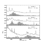
Figure 2.— The spectral signature, $\Delta\log F_{\lambda}$, due to a change of $\Delta[\rm{m/H}]=-0.1$ dex at three different values of $T_{eff}$ (solid curve in each panel), compared with a measure of the strength of the absorption due to various ions of Fe (shaded regions). In particular, the shaded regions show the total values of $gf$ for all the Fe transitions within each ATLAS 9 wavelength bin, arbitrarily scaled and shifted for display. The figure demonstrates that, in the UV region and within the temperature range of the B stars, the overall signature of changes in the “metallicity” of an ATLAS 9 model is mainly due to one particular element — Fe. Other elements contribute within much more restricted wavelength regions, such as Mg II $\lambda 2800$ (in the $T_{eff}=10000$ K case) or Si IV $\lambda 1400$ and C IV $\lambda 1550$ (both in the $T_{eff}=30000$ K case). The strong features in $\Delta\log F_{\lambda}$ at 2325 Å and 2495 Å in the 20000 K and 30000 K panels, respectively, are spurious model features which correspond to no observed stellar lines (see §3).

Figure 3.— The dereddened FOS energy distribution of BD+33^∘ 2642 from 1150 Å to 8000 Å is shown (solid circles) along with the best-fitting ATLAS 9 model (solid histogram line). Crosses indicate data points excluded from the fit, due to contamination from interstellar gas-phase absorption lines, spurious model points, and emission in the stellar H$\alpha$ and H$\beta$ lines. The inset shows an expanded view of the region surrounding the Balmer jump. The parameters of the model are given in Table 2; the $R(V)=3.1$ extinction curve from F99 was used. Over the wavelength range shown, the deviations between the model and the data are typically less than 2$\%$.

Figure 4.— Sample fits for lightly reddened stars. Dereddened energy distributions for 10 main sequence stars ranging from spectral type O9.5 to A0 V are shown (symbols) along with the best-fitting ATLAS 9 models (solid histogram lines). Crosses indicate data points excluded from the fits. The parameters of the models are given in Table 2; the $R(V)=3.1$ extinction curve from F99 was used. The Johnson and Strömgren photometry data have been converted to flux units for display only. The fitting procedure utilizes only the UV fluxes and the $V$ magnitude. The $U$ band point appears high in stars with large Balmer jumps because its broad band straddles the jump. The logarithmic fluxes have been arbitrarily displaced vertically for display purposes. The offsets applied are, from top to bottom, 14.22, 13.59, 13.80, 13.41, 12.03, 12.08, 11.78, 10.06, 10.90, and 10.26

Figure 5.— Best-fitting ATLAS 9 models for HD 172167 (Vega; top) and HD 72660 (bottom). The symbols are the same as in Fig. 4 and the same reddening model was used. The fit for Vega is relatively poor between $1200<\lambda<1500$ Å, possibly due to carbon opacity unaccounted for by the model (see text). Both stars have similar temperatures and surface gravities, and their energy distributions differ primarily because of their different Fe abundances (see Table 2).

Figure 6.— Best-fitting ATLAS 9 model and UV/optical extinction curve for HD 147933 ($\rho$ Oph). The top panel shows the observed IUE plus optical energy distribution (symbols same as in Fig. 4). The middle panel shows the dereddened energy distribution along with the best-fitting ATLAS 9 model. The parameters of the model are given in Table 2. The dereddened energy distribution was also corrected for the effects of interstellar Ly $\alpha$ absorption, assuming a column density of $N({\rm H}\/I)=4.27\times 10^{21}$ cm^-2 from Diplas & Savage 1994. The lower panel shows the normalized UV extinction curve determined by the fitting procedure (thick solid line) overplotted on the actual normalized ratio of the best-fitting model to the observed (but Ly $\alpha$-corrected) SED (filled circles). For comparison, the normalized extinction curve for HD 147933 derived by FM using the traditional pair method (dotted line) and the average Galactic curve for $R(V)=3.1$ from Fitzpatrick 1999 (dash-dot line) are also shown.

References

- Aannestad (1995) Aannestad, P.A. 1995, ApJ, 443, 653
- Anderson (1985) Anderson, L.S. 1985, ApJ, 298, 848
- Anderson (1989) Anderson, L.S. 1989, ApJ, 339, 558
- Anderson & Grigsby (1991) Anderson, L. & Grigsby, J.A. 1991 in “Stellar Atmospheres: Beyond Classical Models” eds., L. Crivellari, I. Hubeny & D.G. Hummer (NATO ASI Series, Kluwer Academic Press: Boston), p 365
- Azusienis & Straizys (1969) Azusienis, A. & Straizys, V. 1969, Soviet Astron. A. J., 14, 316
- Bevington (1969) Bevington, P.R. 1969, Data Reduction and Error Analysis for the Physical Sciences (New York: McGraw-Hill)
- Bless & Percival (1997) Bless, R.C., & Percival, J.W. 1997, in Proc. IAU Symp. 189, “Fundamental Stellar Properties”, eds. Bedding, Booth, and Davis (Dordrecht: Kluwer), p. 73
- (8) Boggess, A., et al. 1978a, Nature, 275, 372
- (9) Boggess, A., et al. 1978b, Nature, 275, 377
- Bohlin et al. (1995) Bohlin, R.C., Colina, L., & Finley, D.S. 1995, AJ, 110, 1316
- Bohlin (1996) Bohlin, R.C. 1996, AJ, 111, 1743
- Böhm-Vitense (1985) Böhm-Vitense, E. 1985, ApJ, 296, 169
- Buser & Kurucz (1978) Buser, R. & Kurucz, R.L. 1978, A&A, 70, 555
- Cardelli et al. (1989) Cardelli, J.C., Clayton, G.C., & Mathis, J.S. 1989, ApJ, 345, 245
- Castelli & Kurucz (1994) Castelli, F., & Kurucz, R. L. 1994, A&A, 281, 817
- Code et al. (1976) Code, A.D., Davis, J., Bless, R.C., & Hanbury-Brown, R. 1976, ApJ, 203, 417
- Colina & Bohlin (1994) Colina, L., & Bohlin, R.C. 1994, AJ, 108, 1931
- Cugier et al. (1996) Cugier, H., Burghardt, M., Nowak, D. & Polubek, G. 1996 in “Science With the Hubble Space Telescope – II”, eds. P. Benvenuti, F.D. Macchetto, & E.J. Schreier, p. 432
- Cuhna & Lambert (1994) Cuhna, K. & Lambert, D.L. 1994, ApJ, 426, 171
- Diplas & Savage (1994) Diplas, A., & Savage, B.D. 1994, ApJS, 93, 211
- Dufton (1998) Dufton, P. 1998, in “Boulder-Munich II: Properties of Hot, Luminous Stars”, ed. Ian Howarth, ASP Conference Series Vol. 131, p. 169
- Finley & Koester (1991) Finley, D.S., & Koester, D. 1991, BAAS, 23, 907
- Fitzpatrick (1999) Fitzpatrick, E.L. 1999, PASP, 111, 63 (F99)
- Fitzpatrick & Massa (1990) Fitzpatrick, E.L. & Massa, D. 1990, ApJS, 72, 163 (FM)
- Geis & Lambert (1992) Geis, D.R. & Lambert, D.L. 1992, ApJ, 387, 673
- (26) Grevesse, N., & Anders, E. 1989 in Cosmic Abundances of Matter, ed. C.J. Waddington (New York: AIP), 1
- (27) Grevesse, N., & Noels, A. 1993 in Origin and Evolution of the Elements, eds. N. Prantzos, E. Vangioni-Flam, & M. Cassé (New York: Cambridge University Press), p. 14
- Grigsby et al (1992) Grigsby, J.A., Morrison, N.D., & Anderson, L.S. 1992, ApJS, 78, 205
- Guinan et al. (1998) Guinan, E.F., et al. 1998. ApJ, 509, L21
- Gummersbach et al (1998) Gummersbach, C. A., Kaufer, A., Schaefer, D. R., Szeifert, T., & Wolf, B. 1998, A&A, 338, 881
- Hauck & Mermilliod (1990) Hauck, B. & Mermilliod, M. 1990, A&AS, 86, 107
- Hayes (1985) Hayes, D.S. 1985, in Proc. IAU Symp. 111, “Calibration of Fundamental Stellar Quantities”, eds. D.S. Hayes, L.E. Passinetti, & A.G.D. Philip (Dordrecht: Reidel) p. 225
- Hill & Landstreet (1993) Hill, G.M. & Landstreet, J.D. 1993, A&A, 276, 142
- Kurucz (1991) Kurucz, R.L. 1991, in “Stellar Atmospheres: Beyond Classical Models”, eds. L. Crivellari, I. Hubeny, and D.G. Hummer (Boston: Kluwer) p. 441
- Kudritzki (1992) Kudritzki, R.P. 1992, A&A, 266, 395
- Leitherer et al. (1996) Leitherer, C. et al. 1996, PASP, 108, 996
- Malagnini et al. (1983) Malagnini, M.L., Faraggiana, R., & Morossi, C. 1983, A&A, 128, ls375
- massa (1987) Massa, D. 1987, AJ, 94, 1675
- massa (1989) Massa, D. 1987, A&A, 224, 131
- Massa & Fitzpatrick (1986) Massa, D. & Fitzpatrick, E.L. 1986, ApJS, 60, 305
- Massa & Fitzpatrick (1999) Massa, D. & Fitzpatrick, E.L. 1999, ApJS, submitted (MF99)
- Massa et al (1992) Massa, D., Shore, S.N., & Wynne, D. 1992, A&A, 264, 169
- Mermilliod (1987) Mermilliod, J.C. 1987, A&AS, 71, 413
- Napiwotzki et al. (1994) Napiwotzki, R., Heber, U., & Koeppen, J. 1994, A&A, 292, 239
- Nichols & Linsky (1996) Nichols, J.S., & Linsky , J.L. 1996, AJ, 111, 517
- Relyea & Kurucz (1978) Relyea, L.J. & Kurucz, R.L. 1978, ApJS, 37, 45
- Remie & Lamers (1982) Remie, H. & Lamers, H.J.G.L.M. 1982, A&A, 105, 85
- Rolleston et al. (1996) Rolleston, W.R.J., Brown, P.J.F., Dufton, P.L. & Howarth, I.D. 1996, A&A, 315, 95
- (49) Roundtree, J., & Sonneborn, G. 1993, NASA RP-1312
- Smartt & Rolleston (1997) Smartt, S.J., & Rolleston, W.R.J. 1997, ApJ, 481, L47
- Simonneau (1973) Simonneau, E. 1973, A&A, 29, 357
- Swings et al. (1973) Swings, J.P., Jamar, C. & Vreux, J.M. 1973, A&A29, 207
- Underhill et al. (1979) Underhill, A.B., Divan, L., Prevot-Burnichon, M.-L.,& Doazan, V. 1979, MNRAS, 189, 601
- Varenne (1999) Varenne, O. 1999, A&A, 341, 233
- Walborn et al. (1995) Walborn, N.R., Parker, J.W., & Nichols, J.S. 1995, NASA RP-1363