The pendulum dilemma of fish orbits

Abstract

The shape of a galaxy is constrained both by mechanisms of formation (dissipational vs. dissipationless) and by the available orbit families (the shape and amount of regular and stochastic orbits). It is shown that, despite the often very flattened shapes of banana and fish orbits, these boxlet orbits generally do not fit a triaxial galaxy in detail because, similar to loop orbits, they spend too little time at the major axis of the model density distribution. This constraint from the shape of fish orbits is relaxed at (large) radii where the density profile of a galaxy is steep.

1 Introduction

Destruction of box orbits and growth of chaos in triaxial potentials with a divergent central force are the classical arguments for adopting axial symmetry in modeling galactic nuclei (Binney & Gerhard 1985). The role of the so-called boxlet orbits is comparatively less understood theoretically. These centro-phobic orbits, named after various food families such as bananas, fishes and pretzels (Miralda-Escudé & Schwarzschild 1989), are flattened in a way grossly similar to that of the box orbits in a cored potential, but for reasons not entirely clear they appear not as useful as box orbits when it comes to fit a flattened galaxy model. Pfenniger & de Zeeuw (1989) suspected this is because a closed banana orbit comes in only a limited range of axis ratios. Schwarzschild (1993) suggests the reason being that the boxlets have their density maxima at the turning points (corners) rather than on the major axis. Similar qualitative arguments include that a thick banana orbit and its mirror image together have twice as many corners as a box orbit, which makes them less flexible in fitting a smooth density model (Kuijken 1993). Syer & Zhao (1998) studied banana orbits in the separable non-axisymmetric disc models of Sridhar & Touma (1997), and found that the self-consistency is first broken down near the symmetry axes of the model.

The present analysis is also motivated by the question: what are the main factors in preventing a galaxy being triaxial? Commonly one might attribute to (a) a dissipational formation of a rotation-supported galaxy, or (b) the growth of stochasticity and shrinking of available phase space for low resonance boxlet orbits in triaxial models once a steep cusp or a central blackhole is developed. If these were the only factors, one would expect that if any strongly triaxial models exist, they should be the ones with zero stochasticity and a shallow cusp. Yet Syer & Zhao found that the continuous family of banana orbits in the fully separable discs of Sridhar & Touma cannot make a self-consistent flattened model (density flattening of about $0.6$) even when the surface density profile is as shallow as $R^{-0.01}$. On the other hand Schwarzschild (1993) and Merritt (1997) studied models with a E6 flattening and a much steeper $R^{-1}$ projected cusp and found that they are nearly self-consistent despite large stochasticity in the phase space in non-separable models. There is clearly a third factor in determining the shape of a model, which is (c) the shape of low resonance boxlet orbits. The mismatch of the shape of banana orbits excludes them as suitable orbits for building a triaxial model even when there are unrestricted number of them (Syer & Zhao 1998). Same can be said about loop orbits. A fish orbit, with one of its apocenters aligned with the major axis, is arguably ideal for building a self-consistent model, but somewhat puzzlingly they are populated merely at the level of 20% in Schwarzschild (1993) models. Their role has not been studied in recent literature as detailedly as the banana orbits and the stochastic orbits. Currently about a few dozen grid-based numerical models have been built to explore the parameter space of triaxial models, while a few thousand might be adequate, however, this might be just on the edge of present numerical power.

On the analytical front, a recent study by Zhao, Carollo & de Zeeuw (1999) shows that the shape of orbits very near the major axis of a potential is very useful for classifying whether an orbit is helpful or not helpful for building a potential. They solved for the equations of motion infinitely close to the major axis analytically. They found that boxlet orbits are often ill-suited for building the potential because of mismatch of their shape or curvature at the major axis with that of the density model; they are not flat enough. This is rather surprising because these boxlets are often more flattened than that of the model, both in the globally averaged sense. Another surprising result is that the problem of mismatch of curvature of boxlet orbits is more severe for shallow-cusped (but not cored) systems than for steep-cusped systems; this goes differently from the expected trend from numerical studies if the stochasticity is the main factor in limiting galaxy shapes. However, their analysis is rigorous only for 2-dimensional scale-free non-axisymmetric discs.

Here we seek to highlight the generic problem of boxlet orbits at the major axis (§1.1). We then limit ourselves to fish orbits, but extend the analytical method of Zhao et al. to a general triaxial potential (§2). This allows us to explore the full range of triaxial models of galactic nuclei and judge whether fish orbits are well-suited or ill-suited for building a specific model. Finally we make the connection of our results with properties of observed galaxies and with previous works (§3) and present our conclusions (§4).

1.1 General problem of boxlets and loops: pendulum dilemma

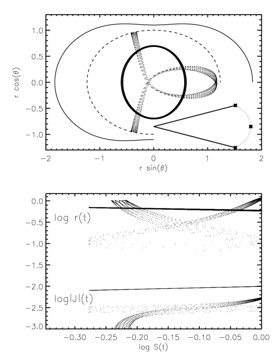
Figure 1: The upper panel shows two types of centro-phobic orbits: a loop orbit (thick filled band) and a fish orbit (dots) together with the iso-density and iso-potential contours (heavy solid and dashed lines respectively). The lower panel shows the radius $r(t)$ and angular momentum $|J(t)|$ of a star vs. the shape function ${\cal S}(r(t),\theta(t),\psi(t))\equiv\rho(r(t),\theta(t),\psi(t))/\rho(r(t),\pi/2,\pi/2)$ along the same two orbits, where each dot is one time step of the orbit and ${\cal S}(t)\rightarrow 1$ as the orbit approaches the major axis. A pendulum with a variable length is also sketched in the upper panel. Note that $|J(t)|$ peaks, hence the star spends least time, at the major axis for boxlets, like it does for loops and the pendulum. They are thus ill suited for building a flattened model unless the model density along the orbit $\rho((r(t),\theta(t),\psi(t))$ is in fact at a minimum on the major axis which could happen if $\rho(r,\theta,\psi)$ falls steeply with radius and the major axis is an apocenter.

The major axis of a model is always where the amplitude of the angular momentum of a regular orbit $J(t)$ reach a local maximum. This is determined by the equations of motion: the torque from the flattened potential always increases the angular momentum when the orbit comes close to the major axis, and decreases it when leaving the major axis. The situation is analogous to a pendulum oscillating around the major axis (see Fig. 1), which never spends enough time near the desired position (the major axis), and always too much time near the undesired positions (the turn-around points). Hence while stars need to slow down so as to spend more time near the major axis to fit the model, the equations of motion tell them to do the opposite. This is perhaps the main limiting factor when boxlet orbits and loop orbits are used in making models (Zhao et al. 1999).

The best that we can do to prolong the stay of a star near the major axis is to let the star reach its apocenter (a local maximum in radius) at the major axis, for example, as in the case of a fish orbit (Fig. 1) or the like such as the $3:4$ pretzels. The situation is analogous to a pendulum with a variable length, e.g., a spring attached by a weight becomes longer at the equilibrium point, and moves slower in terms of the angular speed. Nevertheless the following arguments show that the effect is still limited. To be specific we concentrate on the fish family, but the same arguments apply equal well to any boxlet family with an apocenter on the major axis.

2 Can fishes get out of the pendulum dilemma?

Consider a general triaxial model with a density $\rho(r,\theta,\psi)$ and potential $\Phi(r,\theta,\psi)$ in a spherical coordinate $(r,\theta,\psi)$ where the short axis (z-axis) is the pole with $\theta=0$, and the azimuthal angle $\psi$ runs from $0$ in the $yz$ plane to ${\pi\over 2}$ in the $xz$-plane. Define the parameters $\epsilon_{\theta}$ and $\epsilon_{\psi}$

$$\epsilon_{[\theta,\psi]} \equiv {\partial_{[\theta,\psi]}^{2}\Phi\over 2r\partial_{r}\Phi}|_{r=r_{0},\theta={\pi\over 2},\psi={\pi\over 2}},$$ (1)

so that they describe the flattening of the potential in the $xz$ and $xy$ planes at radius $r_{0}$ on the major axis (x-axis with $\theta=\psi={\pi\over 2}$); generally $\epsilon_{\theta}>\epsilon_{\psi}>0$ since the contours are flatter in the $xz$ plane than the $xy$ plane.

Now launch a fish orbit tangentially from its major-axis apocenter at radius $r_{0}$ with an angle (pitch angle) $\chi$ from the $xy$ plane and an instantaneous angular momentum $J_{0}$. Let the time $t=0$ at the launching, then the trajectory can be approximated as

$$\left[\theta(t),~{}\psi(t)\right] \approx {\pi\over 2}+\left[\cos\chi,~{}\sin\chi\right]\left({J_{0}\over r_{0}v_{c}}\right)\left(t\over T\right)$$ (2)

$$r(t) \approx r_{0}\left[1-\left({1\over 2}-{J_{0}^{2}\over 2r_{0}^{2}v_{c}^{2}}\right)\left({t\over T}\right)^{2}\right],$$ (3)

$$J(t) \approx J_{0}\left[1-{\epsilon_{\theta}\cos^{2}\chi+\epsilon_{\psi}\sin^{2}\chi\over 2}\left({t\over T}\right)^{2}\right]$$ (4)

for a short enough period of time with $t\ll T\equiv{r_{0}\over v_{c}}$, where $T$ is the local dynamical time scale and $v_{c}^{2}\equiv r\partial_{r}\Phi(r,\theta,\psi)|_{r=r_{0}}$ is the local circular velocity squared. The convex dependence of time for both $J(t)$ and $r(t)$, meaning that $t=0$ is a maximum, is a result of the torque from the flattened potential and our choice of the apocenter.

As in the Schwarzschild (1979) method we compute the amount of time that an orbit spends in a set of cells and compare it with the amount of mass in the cell as prescribed by the volume density model. First we divide the density model into shells with equal logarithmic intervals radially ($\eta=\Delta\log r$). Then tessellate the angular dimension into equal solid angles with a size $\Delta\Omega=\beta^{2}$, where $\beta$ is the typical angular scale of the cell. Hence the amount of mass in the cell,

$$\Delta M=\rho(r,\theta,\psi)r^{3}\eta\Delta\Omega\propto r^{2-\gamma_{\mu}}{\cal S}(\theta,\psi),~{}~{}~{}1+\gamma_{\mu}\equiv\left|{\partial\log\rho\over\partial\log r}\right|,$$ (5)

where the volume density $\rho(r,\theta,\psi)$ is approximated as a power-law of slope $1+\gamma_{\mu}$ near radius $r$, and the angular shape of the volume density is specified by a shape function ${\cal S}(\theta,\psi)$. We shall pretend that $\gamma_{\mu}$ is a constant in the subsequent derivation (as in a scale-free model), but generalize it to be a shallow function of $r$ at the end; in the same spirit we treat the flattening parameters $\epsilon_{\theta}$ and $\epsilon_{\psi}$ of the potential model.

Now our orbit crosses the cells with an angular velocity $\omega(t)$ so the amount of time $\Delta t$ that it typically spends in the cell with a characteristic angular size $\beta$ is given by

$$\Delta t={\xi\beta\over\omega},~{}~{}~{}\omega(t)={J(t)\over r^{2}(t)},$$ (6)

where $\xi$ is a geometrical constant of order unity and $J(t)$ is the instantaneous value of the amplitude of the total angular momentum of the orbit when crossing the cell. Here we have ignored the possibility that our orbit may cross a cell radially by arguing that a fish orbit takes much less time to cross a cell tangentially than radially.

Comparing $\Delta t$ with the mass in the cell $\Delta M$, we find that the ratio of the two for an orbit $[r(t),\theta(t),\psi(t)]$ is given by

$${\Delta t\over\Delta M}\propto{\sigma(t)\over{\cal S}(\theta(t),\psi(t))},~{}~{}~{}\sigma\equiv{r^{\gamma_{\mu}}(t)\over J(t)},$$ (7)

where $\sigma(t)$ can be taken as the effective projected density of a fish orbit in the direction $[\theta(t),\psi(t)]$. The important thing here is that while ${\cal S}(\theta(t),\psi(t))$ is generally at maximum on the major axis for any realistic density model, the projected density of a fish orbit $\sigma(t)$ can actually be at minimum at the same place if

$${{\rm d}^{2}\log\sigma(t)\over{\rm d}t^{2}}=\left(\epsilon_{\theta}\cos^{2}\chi+\epsilon_{\psi}\sin^{2}\chi\right)-\gamma_{\mu}\left(1-{J_{0}^{2}\over r_{0}^{2}v_{c}^{2}}\right)$$ (8)

is positive or zero, where we have substituted in eqs. (3) and (4). In other words a fish orbit will be a “bad” orbit if its angular momentum is high with

$${J_{0}^{2}\over r_{0}^{2}v_{c}^{2}}\geq 1-{{\rm Max}[\epsilon_{\psi},\epsilon_{\theta}]\over\gamma_{\mu}}.$$ (9)

Eq. (9) is in fact generally applicable for spotting “bad” orbits. For example, it predicts that loop orbits are universally “bad” since they always visit the major axis with an angular momentum $J_{0}$ slightly greater than that of a circular orbit, $r_{0}v_{c}$.

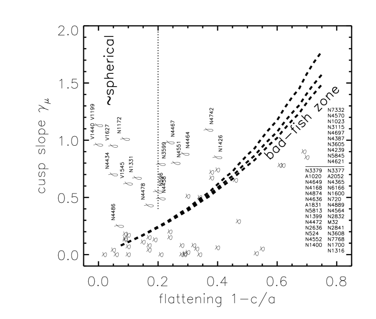
Figure 2: The parameter space for scale-free ellipsoids: the cusp-slope $\gamma_{\mu}$ versus the flattening $1-c/a$. Overplotted (fish-like symbols) are the projected central cusp slope vs. ellipticity of 56 Space Telescope observed galaxies taken simply from the “typical” values given in tabulated form in Faber et al. (1997). Three dashed curves, in descending order, are for triaxiality parameter ${a^{2}-b^{2}\over a^{2}-c^{2}}=[0.9,0.5,0.1]$; they mark the boundary of the “bad-fish zone” (cf. eq. 9). Galaxies marked by the fatter fish symbols (those near or to the right of the dashed lines) are unlikely to host fish orbits which spend enough time on the major axis; their names are listed in the order of cusp slope and ellipticity with ones to the left right being “cored” and rounder than E2. Galaxies to the left of the vertical (dotted) line are very round models; the chance for a highly triaxial and highly flattened galaxy to project into the range left of the vertical line is fairly small; the probability is less than 3% for a galaxy with intrinsic axis ratio $(1:0.75:0.5)$ to appear rounder than E1 and only 10% to appear rounder than E2 in projection from a random orientation. Between the dotted line and the dashed lines is a grey zone where it is more difficult to predict the effect of the fishes.

Our result on fish orbits can also be casted to an even simpler form: eq. (9) is always satisfied with a positive l.h.s. and a negative r.h.s. if $\epsilon_{\theta}>\gamma_{\mu}$, i.e., the iso-potential contours is flatter than what fish orbits can support. This region is marked as “bad-fish-zone” in Fig. 2.

3 Implications to observed galaxies and comparison with previous works

Where are observed galaxies in Fig. 2? One tricky point of connecting our result with observation is that the orientation and intrinsic semi-axes of their three principal axes (assuming a triaxial model) are often unobservable. Nevertheless we can set useful limits since projected contours can only be rounder than intrinsic and their projected central cusp slope is generally equal to or slightly steeper than the cusp-slope $\gamma_{\mu}$ as rigorously defined in eq. (5), i.e., deprojection would shift the fish-like symbols in the scatter diagram down and to the right (roughly the direction pointed by the fish symbols), deeper into the “bad-fish zone”. About half of the galactic nuclei sample are in this zone where fish orbits are “bad” for making a self-consistent triaxial model.

Another tricky point is that the density profiles of real galaxies steepen towards large radii. Giant ellipticals, for example, have a volume density power-law slope $1+\gamma_{\mu}$ in the range of $0-1.3$ in the nucleus, and $2-4$ at radii comparable to one effective radius. Early studies (e.g., Binney 1978) of the kinematics and isophotes of these systems argue convincingly that they are generally triaxial objects, at least outside the nucleus, supported by radial anisotropy from box or boxlet orbits (Schwarzschild 1979). If we let $\gamma_{\mu}$ vary with radius, our result (eq. 9) would suggest that a fish orbit is more effective in providing the anisotropic support to the potential at large radii when the density profile is steeper and the iso-potential contour is rounder than at small radii.

Ryden (1999) in a recent preprint on statistical study of isophotes of a similar galaxy sample came to the conclusion that while isophotes at the inner core of giant ellipticals are consistent with them being randomly oriented oblate objects, the shapes become non-oblate at sufficiently large radii where the mixing of stochastic orbits is incomplete over a Hubble time (Merritt & Valluri 1996). It is reassuring to see both stochastic orbits and fish orbits follow the same general trend, i.e., they seem to be more helpful for supporting a triaxial potential at large radii than at small radii.

Previous numerical studies of scale-free models by Schwarzschild (1993) and double-power-law models by Merritt (1997) with an inner volume density cusp $1+\gamma_{\mu}=2$ show that boxlet orbits cannot support an ellipsoidal model flatter than $E6$ or $E7$. We find that these models are indeed too flat for fish orbits (cf. Fig. 2).

It is less clear whether boxlets become more helpful or less helpful for triaxial models with a shallow cusp. While Merritt & Fridman (1997) suggest that shallow cusp triaxial systems are easier to build than steep cusp systems by extrapolating the findings of two ellipsoidal double-power-law models (with $1+\gamma_{\mu}=1$ or $2$ at the center), our result (eq. 9) predicts that fish orbits become “worse” when the density profile becomes shallow ($1+\gamma_{\mu}\leq 1$). Similarly, while Schwarzschild (1979) finds that triaxial models with a core and a finite force at the center can be built with centro-philic box orbits, Syer & Zhao (1998) find that separable non-axisymmetric disc models with an E5 shape in potential cannot be made with banana orbits even if the projected density profile is as shallow as $R^{-0.01}$. Using a similar analysis, Zhao et al. (1999) also found that the curvatures of boxlet orbits at the major axis could not reproduce that of a 2-dimensional scale-free non-axisymmetric disc if the power-law slope of the disc is small but non-zero. They suggest the existence of a forbidden-zone, very similar to our “bad-fish-zone”. Whether the above findings are contradicting remains to be studied. It depends on whether fish orbits or banana orbits are essential for building a triaxial galaxy. If they occupy only a very small fraction of the phase space, then one might argue that they are marginally interesting orbits and has little effect on the shape of the galaxy. It also depends on whether it is crucial to include additional constraints coming from fitting density off the major axis and from the amount of phase space allocated to regular orbits vs. that allocated to stochastic orbits; these constraints are not exploited here merely because they are not as easy to tap analytically as the conditions of fish orbits near the major axis.

4 Conclusions

In summary we explore the role of fish orbits analytically in a parameter space much larger than possible with previous techniques. Our technique is extended on the basis of the scale-free disc models of Zhao et al. (1999) to a general potential. We find that fish orbits are generally not suitable for building triaxial models because their tendency to “speed” at the major axis often dominates any gain from putting them at a apocenter on the major axis. In essence centro-phobic fish orbits are just as “bad” as loop orbits in the sense that neither can spend much time at the major axis, which excludes them as helpful orbits for a triaxial model. Since all boxlets and loops suffer the so-called pendulum dilemma (cf. § 1.1), with fish orbits being among the most promising of all boxlet orbits to soften the pendulum dilemma, absence of “good” fishes for some very flattened models imply that we have no “good” orbits left for making these models self-consistent.

The general impression from our result on fish orbits and previous works is that a shallow cusp and absence of chaos do not necessarily allow a triaxial model, and triaxiality is difficult to support for steep cusp systems as well as for shallow cusp systems. If all galaxies have central black holes, then most of the available phase space in a strongly flattened, triaxial potential will be taken by stochastic orbits, loop orbits, and high resonance boxlet orbits. Banana orbits, fish orbits and other low resonance food orbits can come only in limited flavors, i.e., axis ratios and sizes. The lack of a continuous varieties of shapes in the building blocks could be a serious limitation for building a smooth self-consistent models since any model built would likely to show undesirable spiky features reminiscent of the sharp boundaries of individual banana or fish. The mismatch of shapes must be another important limiting factor for triaxial galaxies, in addition to dissipational formation and growth of chaos.

HSZ thanks Tim de Zeeuw for comments on an early version of the paper which helped greatly to improve the presentation here.

References

- [1] Binney J.J., 1978, MNRAS, 183, 501
- [2] Faber S.M, et al., 1997, AJ, 114, 1771
- [3] Gerhard O.E., Binney J.J., 1985, MNRAS, 216, 467
- [4] Kuijken K., 1993, ApJ, 409, 68 (K93)
- [5] Merritt D.R. 1997, ApJ, 486, 102
- [6] Merritt D.R., Fridman T., 1996, ApJ, 460, 136
- [7] Merritt D.R., Valluri M., 1996, ApJ, 471, 82
- [8] Miralda-Escudé J., Schwarzschild M., 1989, ApJ, 339, 752
- [9] Pfenniger D., de Zeeuw P.T., 1989, in Dynamics of Dense Stellar Systems, ed. Dave Merritt, Cambridge Univ. Press, 1989, 81
- [10] Ryden S.B. 1999, ApJ, submitted
- [11] Schwarzschild M., 1979, ApJ, 232, 236
- [12] Schwarzschild M., 1993, ApJ, 409, 563
- [13] Sridhar S., Touma J., 1997, MNRAS, 287, L1
- [14] Syer D., Zhao H.S., 1998, MNRAS, 296, 407
- [15] Zhao H.S., Carollo C.M. & de Zeeuw P.T. 1999, MNRAS, 304, 457