On the CCD Calibration of Zwicky galaxy magnitudes
& The Properties of Nearby Field Galaxies

Abstract

We present CCD photometry for galaxies around $204$ bright ($m_{Z}<15.5$) Zwicky galaxies in the equatorial extension of the APM Galaxy Survey, sampling and area over 400 square degrees, which extends 6 hours in right ascension. We fit a best linear relation between the Zwicky magnitude system, $m_{Z}$, and the CCD photometry, $B_{CCD}$, by doing a likehood analysis that corrects for Malmquist bias. This fit yields a mean scale error in Zwicky of 0.38 mag per magnitude: ie $\Delta m_{Z}\simeq~{}(0.62\pm 0.05)~{}\Delta B_{CCD}$ and a mean zero point of $<B_{CCD}-m_{Z}>=-0.35\pm 0.15$ mag. The scatter around this fit is about $0.4$ mag. Correcting the Zwicky magnitude system with the best fit model results in a 60% lower normalization and $0.35\;{\rm mag}$ brighter $M_{*}$ in the luminosity function. This brings the CfA2 luminosity function closer to the other low redshift estimations (eg Stromlo-APM or LCRS). We find a significant positive angular correlation of magnitudes and position in the sky at scales smaller than about 5 armin, which corresponds to a mean separation of $120h^{-1}\;{\rm Kpc}$. We also present colours, sizes and ellipticities for galaxies in our fields which provides a good local reference for the studies of galaxy evolution.

1 Introduction

Some important aspects of galaxy evolution can only be understood by studying the statistical properties of nearby field galaxies, in particular its luminosity function (LF). As well as providing vital information for galaxy evolution studies, an accurate knowledge of the present day LF is needed to normalize the number counts of galaxies at fainter magnitudes, and to understand the clustering and large scale structure of the galaxy distribution. Moreover, the colour distribution of the nearby galaxies provides a basic reference to determine star formation rates in galaxies.

Much recent work has been directed towards studying the evolution of the LF using samples of faint galaxies at high-redshift, but a consideration of the ensemble of available estimates of the LF at low redshifts suggests that there are still large inconsistencies which must be reconciled before reliable conclusions can be drawn about the implications of deep surveys.

Survey	Band	$N_{gal}$	$\bar{z}$	$M_{*}$	$\alpha$	$\phi_{*}$
						$h^{3}\;{\rm Mpc}^{-3}$
CfA2	$m_{Z}$	9063	0.025	$-18.8\pm 0.3$	$-1.0\pm 0.2$	$0.040\pm 0.01$
SSRS2	$B(0)$	2919	0.025	$-19.5\pm 0.08$	$-1.2\pm 0.07$	$0.015\pm 0.003$
SAPM	$b_{\rm J}$	1658	0.050	$-19.5\pm 0.13$	$-1.0\pm 0.15$	$0.014\pm 0.002$
ESP	$b_{\rm J}$	3342	0.1	$-19.6\pm 0.07$	$-1.2\pm 0.06$	$0.020\pm 0.004$
2dF	$b_{\rm J}$	5869	0.14	$-19.7\pm 0.06$	$-1.3\pm 0.05$	$0.017\pm 0.002$
LCRS	$r$	18678	0.1	$-20.3\pm 0.02$	$-0.7\pm 0.05$	$0.019\pm 0.001$
CS	$R_{KC}$	1762	0.06	$-20.7\pm 0.2$	$-1.2\pm 0.2$	$0.025\pm 0.006$

Table 1: Luminosity Function parameters derived from currently available surveys.

It is common practice to fit the LF to the so called Schechter (1976) form:

$$\phi(L)=\phi_{*}~{}\left({L\over{L^{*}}}\right)^{\alpha}~{}{\rm exp}\left(-{L\over{L^{*}}}\right),$$ (1)

were luminosity is related with magnitude in the usual way, ${L\over{L^{*}}}=10^{0.4(M_{*}-M)}$. Determinations of the low redshift $B$-band LF are available from the Stromlo-APM Survey (SAPM, Loveday et al., 1992), the Southern Sky Redshift Survey (Da Costa et al., 1994), the CfA2 redshift survey (Marzke et al., 1994), and more recently from the ESO Slice Project (Zucca et al., 1997) and the 2dF Galaxy Redshift Survey (Folkes et al., 1999). Determinations in the $R$-band are available from the Las Campanas Redshift Survey (LCRS, Lin et al., 1994) and from the Century Survey (CS, Geller et al., 1997). The best determinations of the Schechter function parameters from each of these surveys are listed in Table 1. The SSRS2 is based on the ESO-Uppsala photometry of Lauberts & Valentijn (1989), but transformed to the $B(0)$ system of Huchra (1976). Da Costa et al. (1994) ascribe the difference in the LFs of the two surveys to the large colour-term used by Lauberts & Valentijn to relate the two systems, and so we therefore use $m_{Z}$ for Zwicky magnitudes and $B(0)$ for SSRS2 magnitudes. Da Costa et al. (1994) quote the $rms$ difference between $B(0)$ and $b_{\rm J}$ as $\mathrel{\hbox to0.0pt{\lower 3.0pt\hbox{$\mathchar 536\relax$}\hss}\raise 2.0pt\hbox{$\mathchar 316\relax$}}0.2\;{\rm mag}$. We quote the results for the red LFs of the Las Campanas and Century surveys here for completeness, and do not concern ourselves with the details of the transformations between red and blue passbands. We note however that Geller et al., 1997 find the LF obtained from the CS to be in excellent agreement with a prediction based on colour transfmorations applied to the SSRS2 LF.

Allowing for this adjustment between blue and red magnitudes, the final six rows of Table 1 are all in reasonable agreement, with only the CfA2 result showing a large deviation, particularly in the value of $\phi_{*}$. The difference in the LFs deduced from the CfA2 and SAPM surveys is illustrated in Figure 1.

Figure 1: Luminosity function estimations in the SAPM and the CfA2 as a function of absolute magnitudes $M$ in each magnitude system ($b_{J}$ or $m_{Z}$). The continuous lines enclose the 2-sigma region in the SAPM estimation whereas the dashed lines enclose the 2-sigma region in the CfA2 estimate.

At face value, the CfA2 LF seems to have less intrinsically bright galaxies (at least 10 times less M=-21 galaxies). Of course, this depends on the transformation between Zwicky $m_{Z}$, APM $b_{j}$ or LCRS $R$ magnitudes. Efstathiou et al. (1988) adopted the relation $m_{Z}=B+0.29$ for the CfA1 survey (Huchra et al. 1983). This transformation would move the CfA2 LF in the correct direction to reconcile it with other measurements, although Lin et al. (1994) point out that a shift of $0.7\;{\rm mag}$ in $M$ is required to reconcile $M_{*}$ with the other surveys. However, a simple shift in the magnitude zero-point would not correct for the apparent discrepancy in the normalisation, which would suggest that a more subtle effect is present in the CfA2 data.

In this paper we present the results of a photometric survey of bright galaxies in the overlap region of CfA2 and the equatorial extension of the APM Galaxy Survey (Maddox et al. 1990a,b; Maddox et al. 1991), which we will use to investigate this apparent discrepancy. In Section 2 we begin by comparing the APM photometry with the Zwicky measurements. We describe our CCD observations in Section 3, and compare our observations with Zwicky’s photometry in Section 4. In Section 5 we give some other properties for the galaxies in our fields and dicuss the implications for the LF. In Section 6 we compare our results with the findings of other authors and discuss the possible implications for other results. No direct CCD calibration has yet been published for this part of the APM Galaxy Survey. We will present a detailed comparison of our CCD photometry with the APM data down to the survey completeness limit in a separate paper.

2 A Comparison of Zwicky and APM magnitudes

From the information used to calibrate the APM survey we would expect $B\simeq b_{\rm J}^{\rm APM}+0.2$, given the mean $(B-V)\sim 0.7$ and the colour equation $b_{\rm J}=B-0.28(B-V)$ (Blair & Gilmore 1982; Maddox et al. 1990b; although this shift could increase by as much as $0.07\;{\rm mag}$ according to the findings of Metcalfe, Fong & Shanks, 1995). Adopting the relation between $m_{Z}$ and $B$ used by Efstathiou, Ellis & Peterson (1988), this transformation would imply

$$m_{Z}\simeq b_{\rm J}+0.5,$$ (2)

which is close to the shift in $M_{*}$ adopted by Lin et al. (1996), and, if taken as they stand, would suggest that the results of the two surveys might be consistent, at least in $M_{*}$.

We investigated the usefulness of this relation by considering the subset of $\sim 100$ galaxies found in the part of the APM Galaxy Survey equatorial extension which overlaps with the Southernmost region of CfA2 (The S+3 sample of Marzke et al., 1994). This sample is drawn entirely from volume V of the Zwicky catalogue. We have used the publically available CfA1 catalogue as our source for Zwicky galaxies, with magnitudes corrected as described in CfA1. The CfA1 includes redshifts only for galaxies with $m_{Z}<14.5$, but has magnitudes and positions for $m_{Z}<15.5$. Marzke et al find this sample to be representative of the whole of the Southern part of CfA2 (their Figure 3). We inspected this sample of galaxies on the film copies of the UKST IIIa-J Sky Survey plates, and examined the image maps as reconstructed from the APM survey data. We removed from our sample all those galaxies which had either been broken up into multiple image components or which were composed of multiple components which had been merged into a single object by the APM software. The distribution of these objects in the $m_{Z},b_{\rm J}$ plane is shown in Figure 2. A simple least squares fit to these data with the slope constrained to be unity gives a zero-point shift of

$$m_{Z}=b_{\rm J}-0.6\pm 0.5,$$ (3)

which is more than a magnitude in the opposite sense to that implied by equation 2. As will be noted below a detailed calibration requires a correction for Malmquist bias.

Figure 2: Comparison of the apparent magnitudes for a sample of $\sim 100$ galaxies in the overlap region of the SAPM and the CfA2. Magnitudes in the SAPM catalogue correspond to APM $b_{J}$ estimations while magnitudes in the CfA2 are Zwicky magnitudes, $m_{Z}$. The continuous line corresponds to $b_{J}=m_{z}$ and the dashed line is the best linear fit, $m_{Z}=b_{J}-0.6\pm 0.5$, showing both an offset and a large scatter. We would expect to find at least $m_{Z}=b_{J}+0.5$

The APM Survey is internally calibrated by matching images in plate overlaps, with the overall zero-point fixed by a number of CCD frames distributed over the survey region (Maddox et al., 1990b). At bright magnitudes ($b_{\rm J}\mathrel{\hbox to0.0pt{\lower 3.0pt\hbox{$\mathchar 536\relax$}\hss}\raise 2.0pt\hbox{$\mathchar 316\relax$}}17$) the calibrations are less well determined due to a combination of variations in galaxy surface brightness profiles and the smaller number of bright galaxies found in the plate overlap regions. The equatorial survey extension has been calibrated by matching to the original survey using plate overlaps and the adopted zero-point for the whole survey taken from the original CCD photometry. Maddox et al. (1990b) also used their CCD frames to perform an internal consistency check on the quality of the plate-plate matching technique, and found the residual zero point errors on individual plates to be $\mathrel{\hbox to0.0pt{\lower 3.0pt\hbox{$\mathchar 536\relax$}\hss}\raise 2.0pt\hbox{$\mathchar 316\relax$}}0.04\;{\rm mag}$. The individual uncertainties in galaxy magnitudes in the APM system are therefore expected to be much smaller than effect shown in Figure 2. It is possible that an improvement in the quality of the plate material used for the more recent plates of the equatorial extension coupled with changes in the plate copying process could result in a small change in the saturation correction required for bright galaxies, and that this could produce an effect in this direction (Maddox, private communication). However, account was taken of such effects in the construction of the equatorial extension, and any residual effect is likely to be much smaller than the discrepancy shown here.

The transformation of Zwicky magnitudes to $B$ deduced by Efstathiou, Ellis & Peterson (1988) are based on a comparison of the CfA1 survey data with the Durham–AAT redshift survey using 139 galaxies (Peterson et al. 1986). These authors find that the different volumes of the Zwicky catalogue have large variations in the zero-points, although volume V is found to be representative of the calibration as estimated from all volumes. These data are limited to $m_{Z}<14.5$, and the luminosity function parameters inferred for the CfA1 are consistent with the parameters listed for the other surveys in Table 1. It is not possible to draw a direct comparison of the APM data with Zwicky data brighter than $m_{Z}\sim 14$, due to heavy saturation of galaxies this bright in the APM data. The most plausible inference from the comparison described above would therefore be a difference in the magnitude scales of the two surveys for $b_{\rm J}\mathrel{\hbox to0.0pt{\lower 3.0pt\hbox{$\mathchar 536\relax$}\hss}\raise 2.0pt\hbox{$\mathchar 318\relax$}}14$, with the calibration of Efstathiou, Ellis & Peterson (1988) being appropriate for the Zwicky system at brighter magnitudes.

3 CCD Data

3.1 Observations

We used the galaxies from the sample discussed in the previous section as the basis for a CCD survey to investigate the above discrepancy by providing an independent calibration for both surveys. This overlap region is essentially defined as $21^{\rm h}50<\alpha<3^{\rm h}40$ and $-0.25^{\circ}<\delta<0.25^{\circ}$. We obtained images with the 2.5m Isaac Newton Telescope(INT) and 1.0m Jacobus Kapteyn Telescope(JKT) in October 1994. The decision to use two telescopes was motivated by the number of close groups of Zwicky galaxies in the region, so that we use the $10^{\prime}$ field of view available at the INT to image cluster fields containing groups of bright galaxies and the $6^{\prime}$ field of view of the JKT to image individual galaxies. We used identical Tektronix $1024\times 1024$ detectors (TEK3 and TEK4) and Harris $B$ and $R$ filters on the two telescopes. We obtained observations of 58 fields in two nights at the INT and 73 fields in three nights at the JKT with exposure times of 360s and 600s, respectively. We observed a number of photometric standards from the list of Landolt (1992), at hourly intervals throughout each night, as well as the field of the Active Galaxy AKN120 which contains a number of photometric standards (Hamuy & Maza, 1989).

The data were reduced using standard techniques as implemented in the IRAF ccdred packages, with the exception that we used a modified version of the overscan correction routine to compensate for a saturation of the preamplifier used with TEK4 on the JKT. This effect manifested itself as a sudden drop in the overscan level following readout of particularly bright stellar objects in the field, and subsequent exponential recovery to the normal level as the next $\sim 100$ rows were read out. We found that this problem could be corrected by fitting the overscan regions on either side of the drop for those fields where the effect occurred.

Extinction coefficients were derived each night, giving values in the range $0.10\leq k_{B}\leq 0.12$. We determined zero-points for the two combinations of telescope and detector to be

$$B_{0,INT}=24.16\pm 0.02,$$ (4)

and

$$B_{0,JKT}=21.77\pm 0.02.$$ (5)

We also obtained $R$-band images of our standards and target fields, with zero points determined to be $R_{0,INT}=24.33\pm 0.1$ and $R_{0,JKT}=22.11\pm 0.02$, but we were unable to determine any significant colour term from our standard stars, consistent with previous experience with this combination of CCD and filters which are designed to be very close to the Johnson–Cousins system.

3.2 Image Detection and Photometry

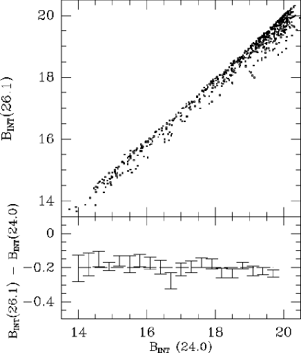
Figure 3: Comparison of total magnitudes $B_{INT}$ for different isophotes: $I=26.1\;{\rm mag\;arcsec}^{-2}$ to $I=24.0\;{\rm mag\;arcsec}^{-2}$.

We used the STARLINK PISA image detection and photometry software for our photometric analysis. This is essentially the same as the image detection software used in the construction of the APM Galaxy Survey (Irwin, 1986). The basic input parameters for the detection are the threshold intensity per pixel or surface brightness, $I_{s}$, and the minimum size of the object to be detected, $A_{s}$. Amongst other parameters PISA returns total area $A_{T}$, the ellipticities and the isophotal magnitude $B_{I}$ or the corresponding total magnitude $B$ resulting from a curve of growth analysis for each detected object after removal of any overlapping objects.

Given that our CCD survey was designed to provide a calibration of both the APM and Zwicky data, we were necessarily interested in a wide range of magnitudes ($14\leq B\leq 20$) and image sizes. For this range of objects there was no unique combination of $I_{s}$ and $A_{s}$ that could deblend the faint objects without breaking the bright ones. In order to automate this process as much as possible for the whole range of magnitudes, we ran PISA several times with different combinations of $I_{s}/A_{s}$. These are listed in Table 2.

	$I_{s}$	$A_{s}$
	$\;{\rm mag\;arcsec}^{-2}$	${\rm arcsec}^{2}$
INT1	26.1	96
INT2	25.7	34
INT3	25.4	34
INT4	25.0	17
INT5	24.6	10
INT6	24.4	10
JKT1	25.0	12
JKT2	24.5	12
JKT3	24.1	6
JKT4	23.7	6
JKT5	22.9	3

Table 2: Input parameter sets used for image analysis.

We chose a larger (smaller) area for the fainter (brighter) isophotes so as to select similar objects in all runs. Objects in the final catalogue were selected from the INT4 and JKT4 runs. The information from different isophotes was then used to perform an automatic rejection of broken or contaminated images. After rejection, the total magnitude and size were the largest remaining estimates of $B$ and $A_{T}$, which typically correspond to the faintest isophote left. The error in $B$ was taken to be the variance in the different estimates for total magnitudes. Objects with rejected isophotes were automatically labeled and checked visually. We refer to total magnitudes estimated in this way as $B_{INT}$ and $B_{JKT}$ for the INT and JKT sets, respectively, or $B_{CCD}$ in general. These effectively correspond to total magnitudes detected at isophotes $26.1\;{\rm mag\;arcsec}^{-2}$ and $25.0\;{\rm mag\;arcsec}^{-2}$, respectively, unless stated otherwise.

To check if our isophotes are low enough we have also computed total magnitudes determined by PISA using higher isophotes. We find a small zero-point shift of the total $B_{INT}$ scale as a function of the isophote $I$, but for a given $I$ this shift is not a function of $B$ over the wide magnitude range considered here. This is illustrated in Figure 3 which shows a change of $\approx 0.2\;{\rm mag}$ in the mean $B_{INT}(I)$ when we change the isophote from $I=26.1\;{\rm mag\;arcsec}^{-2}$ to $I=24.0\;{\rm mag\;arcsec}^{-2}$. Changing the isophote from $I=26.1\;{\rm mag\;arcsec}^{-2}$ to $I=25\;{\rm mag\;arcsec}^{-2}$ introduces a change of only $0.1\;{\rm mag}$. Changing the detection isophote from from $I=26.1\;{\rm mag\;arcsec}^{-2}$ to $I=24.4\;{\rm mag\;arcsec}^{-2}$ also introduces a change in $B_{INT}$ of about $0.2\;{\rm mag}$. We therefore conclude that the residuals associated with our final choice of detection isophote are small compared to the shifts illustrated in Figure 2.

This analysis also implies that there should be a mean zero-point shift in the JKT data relative to the INT data of $0.1\;{\rm mag}$ due to difference in the isophotes used. We therefore apply this shift to all objects observed with the JKT to transform these data to our $B_{26.1}$ system.

Finally, we investigated the possibility that there could be a small effect due to the change in mean redshift of the samples at fainter magnitudes by searching for a change in the mean galaxy colour. Figure 4 shows ($B_{INT}$-$R_{INT}$) as a function of $B_{INT}$. There is only a small colour evolution within the errors. A linear fit to the binned data in Figure 4 yields $B-R=0.016~{}B+1.23$ with a mean $B-R=1.50$ (the mean weighted by each galaxies is $B-R=1.61$ as is dominated by the faint objects).

Figure 4: The top panel shows the red magnitudes $R_{CCD}$ for a subsample of INT galaxies as a function of the blue $B_{CCD}$ ones. The bottom panel shows the colour $B_{CCD}$-$R_{CCD}$ evolution as a function $B_{CCD}$.

4 Comparison with the Zwicky Catalogue

In Figure 5 we show the number counts histograms for the 204 Zwicky galaxies in our sample to the different magnitude systems: Zwicky (top), APM (middle), and CCD (bottom). Comparison of the APM and CCD data shown here suggests that the effect shown in Figure 2 is unlikely to be an artefact of saturation effects in the equatorial APM Survey data at bright magnitudes (see Section 2).

Figure 5: Histograms comparing the numbers of galaxies as a function of apparent magnitude $B$. Each panel shows in black, from top to bottom, the Zwicky, APM and CCD magnitudes for the same objects. In the lower two panels we also show the Zwicky histogram as a background for comparison.

We searched for possible correlations between the magnitude differences, $B_{CCD}-m_{Z}$, and other properties of our sample. The top panel of Figure 6 shows the $B_{CCD}-m_{Z}$ difference as a function of CCD colour $B-R$. The colour of Zwicky galaxies is similar to the mean colour in Figure 4, $B-R\simeq 1.5$ and there is no apparent correlation with $B_{CCD}-m_{Z}$ within the scatter. This is a useful check, as any large differences that were due to processing errors might be expected to show up as objects of extreme colour. The bottom panel of Figure 6 shows the scatter in $B_{CCD}-m_{Z}$ as a function of right ascension. Objects were observed in order of increasing RA on each night of our observing run, and so we would expect temporal drifts to show up as a correlation with RA. Again, there is no evidence of any trend. We also investigated possible variations with Galactic latitude (not shown here), and again found no evidence for trends in our data.

Figure 6: $B_{CCD}-m_{Z}$ as a function of CCD colour $B-R$ (top panel) and right ascention (bottom).

The top panel of Figure 7 shows the $B-m_{Z}$ error as a function of the mean surface brightness for all Zwicky galaxies. Surface brightness is defined here as the ratio of isophotal magnitudes to the area above a threshold of $25.0\;{\rm mag\;arcsec}^{-2}$ in the INT (triangles) and with a threshold of $24.1\;{\rm mag\;arcsec}^{-2}$ in the JKT (circles). The difference in the threshold explains the systematic shift in the bulk value of mean high surface brightness of the JKT images (as we are closer to the galaxy core). As can be seen in the Figure, there is no apparent variation of magnitude error with surface brightness.

The bottom panel of Figure 7 shows the $B-m_{Z}$ error as a function of the sequential run number. This is close to observational time for the INT (triangles) or JKT (circles) when considered separately (in practice, some of the INT and JKT observations were made on the same night). There is no apparent variation of magnitude error with run number.

Figure 7: $B_{CCD}-m_{Z}$ as a function of surface brightness (top panel) and run number or time of observation (bottom).

Figure 8 is the main result of this paper. It shows the Zwicky magnitude error $B_{CCD}-m_{Z}$ as a function of $B_{CCD}$, for all Zwicky galaxies with $B_{CCD}<17.5$. For the Zwicky magnitudes we have used a constant error: $\Delta m_{Z}=0.05\;{\rm mag}$ (as Zwicky quoted magnitudes with a precision of $0.1\;{\rm mag}$). For the CCD data we used the error described in Section 3.2. A very similar trend is found for the separate INT (closed circles) and JKT images (open squares).

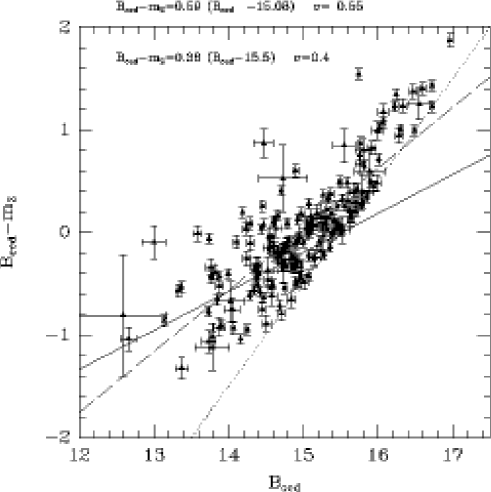
Figure 8: The magnitude error $B_{CCD}-m_{Z}$ as a function of $B_{CCD}$. The dotted line shows the $m_{Z}=15.5$ magnitude limit. The dashed line corresponds to a direct least square fit to the data. The continuous line shows the fit corrected for Malmquist bias (see text).

The dashed line in Figure 8 shows a direct least square fit to the data:

$$B_{CCD}-m_{Z}\simeq 0.6~{}(B_{CCD}-15.1),$$ (6)

which has a scatter of $0.55\;{\rm mag}$.

This fit is the result of the interplay between the scatter in the two magnitude systems and the Zwicky survey limit (shown as dotted line in Figure 8). As a result of this scatter, objects with faint $B_{CCD}$ and bright $m_{Z}$ can be included in the survey, but there is a deficit of objects with faint $m_{Z}$ and bright $B_{CCD}$. i.e. the fit suffers from a Malmquist type of bias. However, for a linear relation, it is apparent that Malmquist bias is insufficient to account for all of the effect shown in Figure 8. We next develop a scheme to correct this fit for the effects of Malmquist bias.

4.1 Malmquist bias correction

Different magnitude system are subject to different systematic errors, and even in the best of the situations intrinsic differences in the morphology, environment and spectrum of the galaxies tend to introduce stochastic fluctuations in any magnitude system. We want to find a best fit linear relation between the Zwicky, ${m_{Z}}$, and CCD, $B_{CCD}$, system:

$$m_{Z}=\lambda B_{CCD}+Z,$$ (7)

where $\lambda$ will account for any scale difference and $Z$ is a zero point shift. In general, both $m_{Z}$ and $B_{CCD}$ are stochastic variables and equation 7 is just a mean relation. As is common practice we will assume that there is Gaussian scatter around the above mean relation (due to the accumulation of multiple uncorrelated factors). That is, given a measured magnitude $m_{Z}$, the error is given by:

$$P(\Delta)={1\over{N}}\,\exp\left[{-{{\Delta^{2}}\over{2\sigma^{2}}}}\right],$$ (8)

where $\Delta\equiv m_{Z}-\overline{m_{Z}}$ is a stochastic variate, $\overline{m_{Z}}$ is some mean best fit value in the linear relation of equation 7, $\sigma$ is the $rms$ error and $N$ is a normalization factor. For a sample that is not magnitude limited we have $N=\sqrt{2\pi}\sigma$. For a magnitude limited sample, where $m_{Z}<m_{Z}^{lim}$, the probability is the same but has a different normalization:

$$N=\int_{-\infty}^{m_{Z}^{lim}-\overline{m_{Z}}}\,dm_{Z}\,\exp\left[{-{{\Delta^{2}}\over{2\sigma^{2}}}}\right],$$ (9)

because not all magnitudes are possible, so that $\Delta\equiv m_{Z}-\overline{m_{Z}}<m_{Z}^{lim}-\overline{m_{Z}}$. Thus, we can write $P(m_{Z})$ in terms of the complementary error function:

$$P(\Delta)={2\,\exp\left[{-{{\Delta^{2}}\over{2\sigma^{2}}}}\right]\over{\sqrt{2\pi}\,\sigma\,{\rm erfc}\left[{\overline{m_{Z}}-m_{Z}^{lim}\over{\sqrt{2}\sigma}}\right]}}\,$$ (10)

so that for $m_{Z}^{lim}=\infty$ we recover the standard Gaussian result.

We are now able to perform a likelihood analysis to find the best fit values of $\lambda$ and $Z$ in the linear relation of equation 7. We define a likelihood as:

$${\cal L}=\prod_{i}P(\Delta_{i})$$ (11)

where $i$ runs over all galaxies in the survey, and:

$$\Delta_{i}=m_{Z}^{i}\,-(\lambda\,B_{CCD}^{i}\,+\,Z)$$ (12)

with $m_{Z}^{i}$ and $B_{CCD}^{i}$ the measured Zwicky and CCD magnitudes for galaxy $i$. In analogy with the standard $\chi^{2}$ test we define a Malmquist bias “corrected chi-square”:

$$\chi^{2}_{Malm}\equiv\sum_{i}\left[{{\Delta^{2}_{i}}\over{2\sigma^{2}}}+2\,{\rm log}({\rm erfc}{\lambda B_{CCD}^{i}+Z-m_{Z}^{lim}\over{\sqrt{2}\,\sigma}})\right]$$ (13)

Note that the measured magnitude errors, $\sigma_{i}$, are added in quadrature to the stochastic error in the linear relation, $\sigma$, which is one of the parameters we want to determine with this fit. The best fit values that we find on maximising the likelihood, using the data in Figure 8, are:

$$\lambda = 0.62\pm 0.05$$ (14)

$$Z = 5.9\pm 0.7$$

$$\sigma = 0.40\pm 0.05,$$

the errors correspond to approximate 99% confidence levels. The values in each uncertainty range are strongly correlated: Lower values of $\lambda$ (eg larger scale errors) are (linearly) correlated with larger values of $Z$, and both are obtained for the smaller $\sigma$. The inverse relation gives:

$$B_{CCD}\simeq 1.61m_{Z}-9.5.$$ (15)

Figure 8 shows as a continuous line the best fit model for the corresponding best fit magnitude difference:

$$B_{CCD}-m_{Z}=(0.38\pm 0.02)(B_{CCD}-15.53)\pm 0.4$$ (16)

Figure 9 shows the residuals of this fit. For comparison we display a Gaussian with same dispersion, $\sigma=0.4$. As mentioned above the Gaussian does not provide a good fit because of the Malmquist bias, which produces a deficit of faint objects. It is not possible to show in this Figure a comparison with the Malmquist bias corrected version for the error probability of equation 10, because this depends not only on the differences, $\Delta$, but also on the measured value, $B_{CCD}^{i}$.

Figure 9: The distribution of magnitude errors from the mean linear fit compared to a Gaussian with dispersion $\sigma=0.4$. The Gaussian does not fit the distribution because of the Malmquist bias, which produces a deficit of faint objects.

Thus, after correcting for the effects of Malmquist bias, the above analysis indicates both a zero-point shift and a change of magnitude scale. The zero point different $Z_{0}$ could be obtained by taking the mean of the magnitude differences over $m_{Z}$ magnitudes (which are the ones that define the survey limit):

$$Z_{0}\equiv<B_{CCD}-m_{Z}>=-0.35\pm 0.15.$$ (17)

which is in good agreement with Efstathiou et al. (1988). The scaling relation between the two magnitude systems is then:

$$\lambda\equiv{\Delta m_{Z}\over{\Delta B_{CCD}}}~{}\simeq~{}0.62~{}\pm~{}0.05.$$ (18)

We can also test the above model for the scale error by estimating the magnitude correlations as a function of projected separation. Figure 10 shows the mean correlation $<\Delta(\theta_{i})\Delta(\theta_{j})>$ as a function of the pair separation $|\theta_{j}-\theta_{i}|$, in arcmin. The uppermost panel shows (as continuous lines) the autocorrelation for magnitude differences in the Zwicky system, $\Delta^{Z}_{i}=m_{Z}^{i}-\overline{m_{Z}}$, where $m_{Z}^{i}$ is the Zwicky magnitude for the $i$th galaxy and $\overline{m_{Z}}=<m_{Z}>$ is the mean Zwicky magnitude in the Survey. The middle panel shows the corresponding autocorrelation for the CCD system: $\Delta_{i}=B_{CCD}^{i}-\overline{B}_{CCD}$. The lower panel shows the autocorrelation of the magnitude errors: $\epsilon_{i}=B_{CCD}^{i}-m_{Z}^{i}$. The long-dashed in each case show the zero values for reference. The short-dashed line in the lower panel shows the prediction based on applying equation 18 to the data, which is extremely close to the observed result.

Figure 10: Mean correlations in magnitude differences $<\Delta(\theta_{i})\Delta(\theta_{j})>$ for pairs of galaxies separated by distance $|\theta_{j}-\theta_{i}|$, in arcmin shown for Zwicky magnitudes (top panel), CCD magnitudes (middle panel), and for the difference $\epsilon$ between Zwicky and CCD magnitudes (lower panel). The short-dashed line shows the prediction using the scale error model $\epsilon=0.6\Delta B$. The long-dashed line shows zero correlation for reference.

We can see in Figure 10 that there is a significant angular correlation between nearby magnitudes and positions with $\theta\mathrel{\mathchoice{\lower 3.6pt\vbox{\halign{$\mathsurround=0pt\displaystyle\hfill#\hfil$\cr<\crcr\sim\crcr}}}{\lower 3.6pt\vbox{\halign{$\mathsurround=0pt\textstyle\hfill#\hfil$\cr<\crcr\sim\crcr}}}{\lower 3.6pt\vbox{\halign{$\mathsurround=0pt\scriptstyle\hfill#\hfil$\cr<\crcr\sim\crcr}}}{\lower 3.6pt\vbox{\halign{$\mathsurround=0pt\scriptscriptstyle\hfill#\hfil$\cr<\crcr\sim\crcr}}}}5^{\prime}$. This correlation is followed by the errors, indicating that the above model is valid. The Zwicky system shows smaller correlations and smaller variance than the CCD system. This can also be understood in the context of the model, as in the Zwicky system the “effective” magnitude scale is about a factor of two smaller (equation 18).

Note that at the typical depth of the survey, ${\cal D}\simeq 80{\,h^{-1}\,{\rm Mpc}}$, the above magnitude correlations are only significant at physical scales smaller than $\mathrel{\mathchoice{\lower 3.6pt\vbox{\halign{$\mathsurround=0pt\displaystyle\hfill#\hfil$\cr<\crcr\sim\crcr}}}{\lower 3.6pt\vbox{\halign{$\mathsurround=0pt\textstyle\hfill#\hfil$\cr<\crcr\sim\crcr}}}{\lower 3.6pt\vbox{\halign{$\mathsurround=0pt\scriptstyle\hfill#\hfil$\cr<\crcr\sim\crcr}}}{\lower 3.6pt\vbox{\halign{$\mathsurround=0pt\scriptscriptstyle\hfill#\hfil$\cr<\crcr\sim\crcr}}}}100\,h^{-1}\,{\rm Kpc}$. This correlation has little effect on typical galaxy clustering scales, $r_{0}\simeq 5{\,h^{-1}\,{\rm Mpc}}$, but might be relevant for the inversion of angular clustering on smaller scales. For example, Szapudi & Gaztañaga (1998) find that on scales $\theta\mathrel{\mathchoice{\lower 3.6pt\vbox{\halign{$\mathsurround=0pt\displaystyle\hfill#\hfil$\cr<\crcr\sim\crcr}}}{\lower 3.6pt\vbox{\halign{$\mathsurround=0pt\textstyle\hfill#\hfil$\cr<\crcr\sim\crcr}}}{\lower 3.6pt\vbox{\halign{$\mathsurround=0pt\scriptstyle\hfill#\hfil$\cr<\crcr\sim\crcr}}}{\lower 3.6pt\vbox{\halign{$\mathsurround=0pt\scriptscriptstyle\hfill#\hfil$\cr<\crcr\sim\crcr}}}}0.1^{\circ}$ there is a significant disagreement between the APM and the EDSGC that is attributed to differences in the construction of the surveys, most likely the dissimilar deblending of crowded fields. At the depth of these Surveys, ${\cal D}\simeq 400{\,h^{-1}\,{\rm Mpc}}$, the above magnitude correlations correspond to $\theta\mathrel{\mathchoice{\lower 3.6pt\vbox{\halign{$\mathsurround=0pt\displaystyle\hfill#\hfil$\cr<\crcr\sim\crcr}}}{\lower 3.6pt\vbox{\halign{$\mathsurround=0pt\textstyle\hfill#\hfil$\cr<\crcr\sim\crcr}}}{\lower 3.6pt\vbox{\halign{$\mathsurround=0pt\scriptstyle\hfill#\hfil$\cr<\crcr\sim\crcr}}}{\lower 3.6pt\vbox{\halign{$\mathsurround=0pt\scriptscriptstyle\hfill#\hfil$\cr<\crcr\sim\crcr}}}}1^{\prime}$ and could also have a significant effect on the angular clustering and its interpretation on these small scales.

4.2 An illustration

An illustration of the scale error in the Zwicky system can be seem in the galaxies shown in Figures 12 and 11. Table 3 gives the Zwicky and CCD magnitudes for each of the Zwicky galaxies as labelled in the Figures. As can be seen from the table, the range of Zwicky galaxies in Figure 11 is $\Delta m_{Z}=0.3$ which is almost 6 times smaller than the CCD range $\Delta B_{CCD}=1.7$. The range for the whole cluster is $\Delta m_{Z}=1.3$, almost a factor of 3 smaller that the CCD range: $\Delta B_{CCD}=3.5$. These illustrations are strongly suggestive of an observer-bias effect, whereby some fainter galaxies are included in the same due to their proximity to brighter objects, e.g. object #9 in Figure 12.

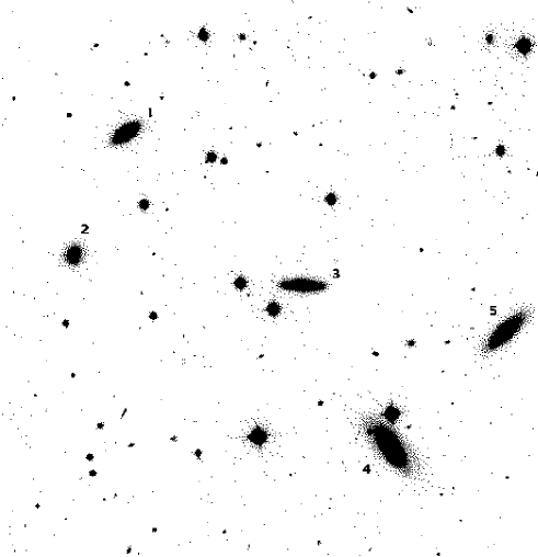
Figure 11: A CCD image (in $B$) containing several Zwicky galaxies (labeled with numbers) in a rich cluster.

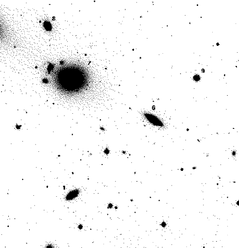
Figure 12: A CCD image (in $B$) containing several Zwicky galaxies (labeled with numbers) in a rich cluster.

Galaxy #	Zwicky $m_{Z}$	CCD $B$
1	15.0	15.0
2	15.0	16.1
3	14.8	15.1
4	14.7	14.4
5	14.8	14.9
6	14.9	14.8
7	14.0	13.2
8	15.2	14.9
9	15.3	16.7

Table 3: Comparison of CCD and Zwicky magnitude for galaxies, as labeled in Figures 11 and  12.

5 The properties of nearby Field Galaxies

We will now present some further properties of the galaxies in our sample: colours, sizes and ellipticities, and discuss the implications for the Luminosity function. This will help us to understand the systematic effects present in the Zwicky magnitude system. As mentioned in § 1, these local properties are interesting in the context of galaxy evolution and star formation rates.

There are still only few samples that are both homogeneous and large enough to provide estimates of the statistical properties of nearby samples, most of which have been selected from photographic plates. Besides the redshift catalogues listed in Table 1, one of the more extensive catalogues of bright galaxies is contained in the Second Reference Catalogue of Bright Galaxies (de Vaucouleurs, de Vaucouleurs & Corwin 1976, known as RC2), which gives magnitudes, colours, ellipticity and morphology for well over a thousand galaxies to a limiting isophote of around $25.0\;{\rm mag\;arcsec}^{-2}$. The problem with this catalogue is that it is a mere compilation of data and was not intended to be complete to any specified limiting magnitude, diameter, or redshift. Moreover it is based on photographic plates.

Our sample is homogeneous enough and extends over a large enough area ( $\simeq 400$ square degrees) to provide a fair sample. Thus the new results based on the CCD magnitudes should be a good local reference for the fainter studies of galaxy evolution.

We will compare the properties of galaxies in the Zwicky ($m_{Z}<15.5$) sample with the corresponding properties of galaxies in the INT fields selected using the CCD blue magnitude $B=B_{CCD}$. We choose two magnitude cuts: $B<16$ which includes most Zwicky galaxies and $19<B<20$, which includes faint galaxies in the same fields.

5.1 Sizes and Ellipticities

Figure 13 shows an histogram of the frequency distribution of galaxies as a function of its area (number of galaxy pixels above detection threshold in the CCD image). Top panel shows Zwicky selected galaxies only. Middle and bottom panels include all the galaxies in the INT fields selected with CCD magnitudes of $B<16$ and $19<B<20$, respectively.

As can be seem in the Figure, Zwicky selected galaxies have a long tail of small objects which is not present in the bright subsample of $B<16$ CCD selected objects. This again illustrates the scale error (and selection biases) in the Zwicky system mentioned above (see also § 6).

The distribution of sizes in logarithmic scale for both CCD sub-samples are well approximated by Gaussians (shown as continuous lines in the figure). The mean size is about $60$ ${\rm arcsec}^{2}$ for $19<B<20$ and $1600$ ${\rm arcsec}^{2}$ for $B>16$, with a rms dispersion of about $20\%$ and $27\%$ respectively (recall that these areas correspond to a nominal threshold of $26.1\;{\rm mag\;arcsec}^{-2}$, fainter thresholds could be needed to sample the size of the lower surphace halos).

Figure 13: Frequency distribution (in per cent) of galaxies as a function of their area (in ${\rm arcsec}^{2}$) for galaxies selected in different ways: (a) Zwicky sub-sample (top), (b) bright galaxies with CCD magnitudes $B<16$ (middle top) and (c) faint galaxies with CCD magnitude $19<B<20$ (middle bottom). (d) area versus ellipticities for all CCD magnitudes $14<B<20$ (bottom).

Figure 14 shows the corresponding frequency distribution for the ellipticities as measure in the galaxy shapes (with a threshold of $26.1\;{\rm mag\;arcsec}^{-2}$). These Figures are in rough agreement with the results by Binney & Vaucouleurs (1982) over the Second Reference Catalogue (RC2).

The local distribution seems remarkably similar to the faint one, given the large differences in sizes shown in Fig.13. This is a good indication that our isophote ($26.1\;{\rm mag\;arcsec}^{-2}$) is low enough, as otherwise we would expect a large excess of round faint objects. There seems to be nevertheless a slight ($\simeq 5\%$) excess of round faint objects. This is probably not due to the seeing (or pixel resolution) as most of the faint objects here have more than 30 ${\rm arcsec}^{2}$ (or 100 pixels) of area (see Fig.13). The lack of correlation between ellipticities $\epsilon$ and areas ${\cal A}$ is illustrated in the bottom panel of Figure 13. A least-square-fit to the points give $\epsilon\simeq 0.277+0.018\log_{10}({\cal A})$.

Figure 14: Frequency distribution (in per cent) of galaxies as a function of their ellipticity for galaxies selected in different ways: (a) Zwicky sub-sample (top), (b) bright galaxies with CCD magnitudes $B<16$ (middle) and (c) faint galaxies with CCD magnitude $19<B<20$ (bottom).

5.2 Colours

Both the morphology and a more detailed study of colours will be presented elsewhere. Here we just show the colour frequencies and discuss some of its implications.

Figure 15 shows the frequency distribution of CCD colour ($B-R$) for all Zwicky galaxies (top) in our sample. We then show the corresponding distributions for the same Zwicky galaxies separated into two sets, corresponding to the JKT (middle) and INT (bottom) CCD frames. As mentioned above, the INT field of view (10’) was larger than the JKT (6’) and so we used the INT to target groups and clusters of galaxies (which could take up several overlaping CCD frames), while the JKT was used for more isolated galaxies. As can be seem in the Figure the INT galaxies are significantly redder, $B-R\simeq 1.57$, than the JKT, $B-R\simeq 1.36$. There are about $\simeq 100$ objects in each subset which roughly corresponds to a random sampling of the total 600 Zwicky galaxies in our survey area (the 600 targets were split in half between the two fields and then more or less randomly selected during each night). The mean colour of our 200 Zwicky galaxies is $B-R\simeq 1.47$. Neither the mean colour or the frequency distribution change significantly when we exclude all the galaxies that are in the same CCD frame (eg to avoid nearby ellipticals). This indicate that selection effects are not important for this distribution.

Given the large area covered (several hundreds of square degree), these results should be a good estimate of the overall mean colour of bright local galaxies. How do these values compare with previous studies? This is a difficult question because it requieres both accurate colours and the accurate fraction of galaxies in different enviroments (eg different morphological types). Previous studies were limited to inhomogeneous samples (eg RC2) or to small numbers of galaxies. For example Kennicutt (1992) presented results for 8 early-type galaxies and 17 spirals to irregulars. Our mean $B-R\simeq 1.47$ can be compared againts the synthetic $B-R$ colours presented by Fukugita et al. (1995). We have used Harris filters which were designed to be very close to the Johnson–Cousins (with $R$ Johnson) system. In these broadbands, Table 3 of Fukugita et al. show $B_{R}=1.67$ for Ellipticals, $1.48$ for S0, $1.2-1.1$ for Spirals and $0.6$ for Irregulars. The range seems in rough agreement with Figure 15, although we find a significant number of objects with $B-R>2$. Notice that these objects are mostly in the INT sample, that is in clusters or groups. While most of the bluer objects with $B-R<1$ are in the JKT fields, that is, they are more isolated (by angular separations larger than $6^{\prime}$, which corresponds to a mean separation larger than $140h^{-1}\;{\rm Kpc}$. Nevertheless, this is seems to be a small effect.

Note that Fukugita et al synthetic colours seem to be slightly less red than the Kennicutt (1992) observations (according to Table 2 in Fukugita et al., they are about 0.1 redder in B-V and this could be larger in B-R). Also notice that we are using total magnitudes, while the synthetic colours are based in small aperture spectra. Galaxies could have quite a different colour distribution (or spectra) in their low-surface halos.

Figure 15: Frequency distribution (in per cent) of galaxies as a function of CCD colour $B-R$ for Zwicky galaxies selected in different ways: (a) All Zwicky in our sample (top), (b) Zwicky galaxies in our JKT sub-sample (middle) (c) Zwicky galaxies in our INT sub-sample (bottom). The same Gaussian distribution is plotted as a solid line in each panel

Figure 16 shows the frequency distribution of CCD colour ($B-R$) for the Zwicky galaxies (top panel) in comparison with the same galaxies selected with CCD magnitudes: with $B<16$ (middle panel) and a sub-set of INT galaxies with $19<B<20$ (bottom panel), which corresponds to the points in Figure 4. The continuous line in all cases shows for reference a Gaussian distribution with mean $B-R=1.45$ and rms deviation of $\sigma=0.4$, which roughly matches the Zwicky frequencies.

It is interesting to notice the peak of local galaxies with $B-R=1.5$ and the spread and shift to the red of the faint objects in the bottom panel. These magnitudes are not k-corrected, which could well explain the relative redening of the faint objects.

Figure 16: Frequency distribution (in per cent) of galaxies as a function of CCD colour $B-R$ for galaxies selected in different ways: (a) Zwicky sub-sample (top), (b) bright galaxies with CCD magnitudes $B<16$ (middle) and (c) faint galaxies with CCD magnitude $19<B<20$ (bottom).

5.3 The local CfA2 Luminosity Function (LF)

Zwicky magnitudes have been used to estimate the LF in the CfA2 redshift catalogue (Marzke et al. 1994). Marzke et al. used a Monte Carlo method to estimate how the LF parameters would change if the dispersion $\sigma_{M}$ were $0.65\;{\rm mag}$ (closer to what we find here than the nominal $0.3\;{\rm mag}$ they used). They found that the true $M_{*}$ should be about $0.6\;{\rm mag}$ brighter, and that a similar conclusion would be reached for a small scale error. Marzke et al. used this estimate to conclude that a combination of incompleteness and a small ($0.2\;{\rm mag}$) scale error would be sufficient to move the CfA2-North values to those found from CfA2-South.

A detailed analysis of the implications of our new Zwicky magnitude calibration on the LF would require the redshift information and this is left for future work. It is nevertheless possible to use the mean relation that we found to show how we expect the LF to change.

In practice, when fitting the Schechter parameters in equation 1 to observational data, the value of $\phi_{*}$ is correlated with the values of $M_{*}$ and $\alpha$. In our case we do not use a fit to data, but just model how the LF changes with an homogeneous linear shift in the magnitude scale. A zero point shift $Z_{0}$ in the magnitude scale, as in equation 17, will just change the value of $M_{*}$:

$$M_{*}(corrected)=M_{*}+Z_{0}.$$ (19)

As the LF measures the number density of galaxies per magnitude inverval, a linear change in the magnitude scale will shift the amplitude of the LF proportionally to the shift in the magnitude interval, i.e. by $\lambda$ in equation (18). Thus we have:

$$\phi_{*}(corrected)=\lambda\,\phi_{*}.$$ (20)

Thus the scale and zero point error in the Zwicky system give the following corrections for the CfA2 South results of Marzke et al. (1994)

$$\phi_{*}(corrected)=\lambda\,\phi_{*}\simeq 0.0124\pm 0.006\,h^{3}\;{\rm Mpc}^{-3}$$ (21)

$$M_{*}(corrected)=M_{*}+Z_{0}\simeq-19.3\pm 0.3.$$ (22)

If applied to the LF for the whole CfA2 survey:

$$\phi_{*}(corrected)=\lambda\,\phi_{*}\simeq 0.025\pm 0.009\,h^{3}\;{\rm Mpc}^{-3}$$ (23)

$$M_{*}(corrected)=M_{*}+Z_{0}\simeq-19.1\pm 0.2,$$ (24)

where we have added the errors in quadrature. Thus the corrected values are now closer the SAPM and LCRS (see Table 1). This can also be seem in Figure 17, where we compare the corrected CfA2 luminosity function given above with the one corresponding to the SAPM. Note that the later is in the APM $b_{J}$ band, so that there could be some additional zero-point shifts between them (see §2).

Figure 17: Luminosity function estimations. The continuous lines enclose the 2-sigma region in the SAPM estimation ($b_{J}$ band) whereas the dashed lines enclose the 2-sigma region in the CfA2 estimation ($B_{CCD}$) after correction for the model of the Zwicky magnitude system and errors. The upper panel shows the corrected LF for CfA2-South, and the lower for the whole CfA2 survey.

6 Conclusion

In this paper we have presented CCD magnitudes for galaxies around $204$ Zwicky galaxies which sample over 400 square degrees, extending 6 hours in right ascension. This subsample is drawn entirely from volume V of the Zwicky catalogue. We find evidence for a significant scale error as pointed out by Bothun & Schommer (1982) and Giovannelli & Haynes (1984). This is found by direct likelihood analysis, corrected for Malmquist bias, and also by noticing the angular correlations between the errors (Fig.10) or the long tail of small objects in the frequency distributions of sizes (Fig.13). The mean scale magnitude error is quite large: $\Delta m_{Z}\simeq~{}0.62~{}\Delta B_{CCD}$, i.e. an error of 0.38 mag per magnitude, while the mean zero point is about $-0.35$ (equation 17), in agreement with Efstathiou et al. (1988).

An illustration of the scale error in the Zwicky system can be seem in the galaxies shown in Figures 12 and 11. These illustrations are strongly suggestive of an observer-bias effect, whereby some fainter galaxies are included in the sample due to their proximity to brighter objects, e.g. object #9 in Figure 12. This bias can also be seem in statistical terms as a long tail of small objects in the frequency distribution of Fig.13.

Huchra (1976) found only a 0.08 mag per magnitude scale error in a callibration of Zwicky galaxies with a photoelectric photometry of 181 sample of Markarian galaxies, which are preferentially spirals. As spiral galaxies are bad tracers of clusters or groups, it is unlikely that these Markarian galaxies include any of the fainter galaxies that contribute to the proximity observer-bias mentioned above (which are mostly ellipticals). This effect would be hard to notice with photoelectric photometry which samples only one object at a time. Note that our analysis is restricted to a narrow range of magnitudes $13.5<m_{Z}<15.5$, as compared to the wider range in Huchra (1976), but this narrow range contains the majority of the galaxies with $m_{Z}<15.5$ and therefore dominates all the relevant statistical properties (such as the luminosity function).

Bothun & Cornell (1990) have studied the calibration of the Zwicky magnitude scale using a sample of 107 spiral galaxies. They suggest that the errors in $m_{Z}$ are minimized if $m_{Z}$ is an isophotal magnitude at $B=26.0\;{\rm mag\;arcsec}^{-2}$, although it is clear from their Figure 2 that even within such a small sample of objects there is a $5\;{\rm mag}$ range of isophotes which give isophotal magnitudes corresponding to $m_{Z}$. This suggests that our isophotal detection limit should be optimal for this comparison.

Takamiya et al. (1995), also with photoelectric photometry, find evidence for a large scale shift between Volume I and Volumes II and V of the Zwicky catalogue. This shift appears to be of order $0.5\;{\rm mag}\;{\rm mag}^{-1}$ over the range $14<m_{Z}<15.7$, which is comparable to our findings for Volume V, although they find very little effect for Volumes II and V. However, we note that Figure 4 of Takamiya et al. shows $B-m_{Z}$ vs. $B$, rather than $m_{Z}$. A similar representation of Figure 8 of this paper looks very similar to Figure 4a of Takamiya et al., which is reasonable, given that Figure 8 implies a strong compression of the $m_{Z}$ axis, which effectively hides the scale error. Unfortunately, the overlap between the 204 objects in our sample and the 155 objects in the Takamiya et al. data is too small to draw any detailed comparison, given that there are $\sim 600$ Zwicky galaxies within the region of our survey.

We have also estimated how this scale error could change the CfA2 luminosity function in §5.3. Figure 17 shows how the corrected estimation is now closer to other local estimates, such as the SAPM. Finally, in §5 we give properties of the galaxies in our sample: colours, sizes and ellipticities, providing one of the largest samples of this kind. The local colour frequency distribution can be well approximated by a Gaussian distribution with mean $B-R=1.45$ and rms deviation of $\sigma=0.40$. These colours compare well with synthetic $B-R$ colours presented Fukugita et al (1995). But there is a significant number of galaxies with $B-R>2$ which are preferably found in clusters and groups, while most of the bluer objects with $B-R<1$ (spirals to irregulars) seem more isolated. These local properties are interesting in the context of galaxy evolution and star formation rates. This will be studied in more detail in future work.

Acknowledgements

The Isaac Newton Telescope (INT) and Jacobus Kapteyn Telescope(JKT) are operated on the island of La Palma by the Isaac Newton Group in the Spanish Observatorio del Roque de los Muchachos of the Instituto de Astrofisica de Canarias. We thank Steve Maddox, Will Sutherland, John Loveday, Cedric Lacey, Michael Vogeley, and Gary Wegner for useful discussions. We also thank the referee for helpful and constructive comments. This work has been supported in part by CSIC, DGICYT (Spain), projects PB93-0035 and PB96-0925, in part by PPARC (UK), and by a bilateral collaboration (Accion Integrada HB1996-0091) between CSIC (Spain) and the British Council (UK). Part of the data reduction and analysis was carried out at the University of Oxford, using facilities provided by the UK Starlink project, funded by PPARC.

7 References

Blair, M., & Gilmore, G., 1982, PASP, 94, 7423

Binney, J., & de Vaucouleurs, G., 1981, MNRAS, 194, 679

Bothun, G.D., & Cornell, M.E., 1990, AJ, 99, 1004

Bothun, G.D., & Schommer, R., 1982, ApJ, 255, L23

Da Costa, L.N., Geller, M.J., Pellegrini, P.S., Latham, D.W., Fairall, A.P., Marzke, R.O., Willmer, C.N.A., Huchra, J.P., Calderon, J.H., Ramella, M., Kurtz, M.J., 1994, ApJ, 424, L1

de Vaucouleurs, G., de Vaucouleurs, A., Corwin Jr., H.G., 1976, Second Reference Catalogue of Bright Galaxies, University of Texas Press, Austin.

Efstathiou, G., Ellis, R.S., & Peterson, B.J., 1988, MNRAS,232, 431

Folkes, S., Ronen, S., Price, I., Lahav, O., Colless, M.M., Maddox, S.J., Deeley, K., Glazebrook, K., Bland-Hawthorn, J., Cannon, R.D., Cole, S.M., Collins, C.A., Couch, W.J., Driver, S.P., Dalton, G.B., Efstathiou, G., Ellis, R.S., Frenk, C.S., Kaiser, N., Lewis, I.J., Lumsden, S.L., Peacock, J.A., Peterson, B.A., Sutherland, W.J., Taylor, K., 1999, MNRAS, 208, 459

Fukugita, M., Shimasaku, K., Ichikawa, 1995, T., PASP, 107, 945

Geller, M.J., Kurtz, M.J., Wegner, G., Thorstensen, J.R., Fabricant, D.G., Marzke, R.O., Huchra, J.P., Schild, R.E., Falco, E.E., 1997, AJ, 114, 2205

Giovanelli, R., & Haynes, M.P., 1984, AJ, 89, 1

Hamuy, M., & Maza, J., 1989, AJ, 97, 720

Huchra, J.P. 1976, A.J,81, 952

Huchra, J.P., Davis, M., Latham, D. & Tonry, J. 1983, ApJS, 52, 89

Kennicutt, R.C., 1992, ApJS, 79, 255

Landolt, A.U., 1992, AJ, 104, 340

Lin, H., Kirshner, R.P., Shectman. S.A., Landy, S.D., Oemler, A., Tucker, D.L., Schechter, P.L., ApJ,464, 60

Loveday, J., Peterson, B.A., Efstathiou, G., & Maddox, S.J., 1992, ApJ,390, 338

Maddox, S.J., Sutherland, W.J., Efstathiou, G., & Loveday, J., 1990a, MNRAS,243, 692

Maddox, S.J., Sutherland, W.J., Efstathiou, G., & Loveday, J., 1990b, MNRAS,246, 433

Maddox, S.J., Sutherland, W.J., Efstathiou, G., & Loveday, J., 1991, in “The Early Observable Universe from Diffuse Backgrounds”, eds. Rocca-Volmerange, B., Deharveng, J.M., & Trân Thanh Vân, J.

Marzke, R.O., Huchra, J.P., & Geller, M.J., 1994, ApJ,428, 43

Metcalfe, N., Fong, R., & Shanks, T., 1995, MNRAS, 274, 769

Peterson, B.A., Ellis, R.S., Efstathiou, G., Shanks, T., Bean, A.J., Fong, R., & Zen-Long, Z., 1986, MNRAS, 221, 233

Schechter, P., 1976, ApJ,203, 297

Szapudi, I., Gaztañaga, E., 1998, MNRAS 300, 493

Takamiya, M., Kron, R.G., & Kron, G.E., 1995, AJ, 110, 1083 A&A,342, 15.

Zucca, E., Zamorani, G., Vettolani, G., Cappi, A., Merighi, R., Mignoli, M., Stirpe, G.M., MacGillivray, H., Collins, C., Balkowski, C., Cayatte, V., Maurogordato, S., Proust, D., Chincarini, G., Guzzo, L., Maccagni, D., Scaramella, R., Blanchard, A., Ramella, M., 1997, A&A, 326, 477

Zwicky, F., Herzog, E., Wild, P., Karpowicz, M., & Kowal, C.T., 1968, Catalogue of Galaxies and Clusters of Galaxies.