AMANDA: status, results and future

presented by Christian Spiering for the AMANDA collaboration:

E. Andres¹¹, P. Askebjer⁴, G. Barouch⁸, S. Barwick⁶, X. Bai¹¹, K. Becker⁹, R. Bay⁵, L. Bergström⁴, D. Bertrand¹², D. Besson¹³, A. Biron², J. Booth⁶, O. Botner¹⁴, A. Bouchta², S. Carius³, M. Carlson⁸, W. Chinowsky¹⁰, D. Chirkin⁵, J. Conrad¹⁴, C. Costa⁸, D. F. Cowen⁷, E. Dalberg⁴, J. Dewulf¹², T. DeYoung⁸, J. Edsjö⁴, P. Ekström⁴, G. Frichter¹³, A. Goobar⁴, L. Gray⁸, A. Hallgren¹⁴, F. Halzen⁸, Y. He⁵, R. Hardtke⁸, G. Hill⁸, P. O. Hulth⁴, S. Hundertmark², J. Jacobsen¹⁰, V. Kandhadai⁸, A. Karle⁸, J. Kim⁶, B. Koci⁸, M. Kowalski², I. Kravchenko¹³, J. Lamoureux¹⁰, P. Loaiza¹⁴, H. Leich², P. Lindahl³, T. Liss⁵, I. Liubarsky⁸, M. Leuthold², D. M. Lowder⁵, J. Ludvig¹⁰, P. Marciniewski¹⁴, T. Miller¹, P. Miocinovic⁵, P. Mock⁶, F. M. Newcomer⁷, R. Morse⁸, P. Niessen², D. Nygren¹⁰, C. Pérez de los Heros¹⁴, R. Porrata⁶, P. B. Price⁵, G. Przybylski¹⁰, K. Rawlins⁸, W. Rhode⁵, S. Richter¹¹, J. Rodriguez Martino⁴, P. Romenesko⁸, D. Ross⁶, H. Rubinstein⁴, E. Schneider⁶, T. Schmidt², R. Schwarz¹¹, A. Silvestri², G. Smoot¹⁰, M. Solarz⁵, G. Spiczak¹, C. Spiering², N. Starinski¹¹, P. Steffen², R. Stokstad¹⁰, O. Streicher², I. Taboada⁷, T. Thon², S. Tilav⁸, M. Vander Donckt¹², C. Walck⁴, C. Wiebusch², R. Wischnewski², K. Woschnagg⁵, W. Wu⁶, G. Yodh⁶, S. Young⁶

1) Bartol Research Institute, University of Delaware, Newark, DE, USA
2) DESY-Zeuthen, Zeuthen, Germany
3) Kalmar University, Sweden
4) Stockholm University, Stockholm, Sweden
5) University of California, Berkeley, Berkeley, CA, USA
6) University of California, Irvine, Irvine, CA, USA
7) University of Pennsylvania, Philadelphia, PA, USA
8) University of Wisconsin, Madison, WI, USA
9) University of Wuppertal, Wuppertal, Germany
10) Lawrence Berkeley Laboratory, Berkeley, CA, USA
11) South Pole Station, Antarctica
12) University of Brussels, Brussels, Belgium
13) University of Kansas, Lawrence, KS, USA
14) University of Uppsala, Uppsala, Sweden

ABSTRACT

We review the status of the AMANDA neutrino telescope. We present results obtained from the four-string prototype array AMANDA-B4 and describe the methods of track reconstruction and neutrino event separation. We give also first results of the analysis of the 10-string detector AMANDA-B10, in particular on atmospheric neutrinos and the search for magnetic monopoles. We sketch the future schedule on the way to a cube kilometer telescope at the South Pole, ICECUBE.

1 The Detector

AMANDA (Antarctic Muon And Neutrino Detector Array) uses the natural Antarctic ice as both target and Cherenkov medium ^?,?). The detector consists of strings of optical modules (OMs) frozen in the 3 km thick ice sheet at the South Pole. An OM consists of an $8^{\prime\prime}$ photomultiplier in a glass vessel. The strings are deployed into holes drilled with pressurized hot water. The water column in the hole then refreezes within 35-40 hours, fixing the string in its final position. In our basic design, each OM had its own cable supplying the high voltage (HV) as well as transmitting the anode signal. For the last 122 OMs deployed in the antarctic season 1998/99, the anode signal drives a LED which’s signal is transmitted via an optical fiber. Other approaches to signal transmission are described in section 6.

Fig. 1 shows the current configuration of the AMANDA detector. The shallow array, AMANDA-A, was deployed at a depth of 800 to 1000 m in 1993/94 in an exploratory phase of the project. Studies of the optical properties of the ice carried out with AMANDA-A showed that a high concentration of residual air bubbles remaining at these depths leads to strong scattering of light, making accurate track reconstruction impossible. Therefore, in the polar season 1995/96 a deeper array consisting of 86 OMs arranged on four strings (AMANDA-B4) was deployed at depths ranging from 1540 to 2040 meters, where the concentration of bubbles was predicted to be negligible according to extrapolation of AMANDA-A results. The detector was upgraded in 1996/97 with 216 additional OMs on 6 strings. This detector of 4+6 strings was named AMANDA-B10 and is sketched at the right side of fig. 1. AMANDA-B10 was upgraded in the season 1997/98 by 3 strings instrumented between 1150 m and 1350 m which fulfill several tasks. Firstly, they explore the very deep and very shallow ice with respect to a future cube kilometer array. Secondly, they form one corner of AMANDA-II which is the next stage of AMANDA with altogether about 700 OMs. Thirdly, they have been used to test new technologies of data transmission.

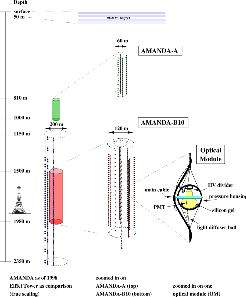
Figure 1: Scheme of the 1998 AMANDA installations. The left picture is drawn with true scaling. A zoomed view on AMANDA-A (top) and AMANDA-B10 (bottom) is shown at the center. The right zoom depicts the optical module.

An essential ingredient to the operation of a detector like AMANDA is the knowledge of the optical properties of the ice, as well as a precise geometry and time calibration of the detector. We make use of the following calibration tools: Pulsed light sources are used to determine a) time offsets, b) the geometry of the array, and c) to derive ice properties. They include a YAG laser calibration system which transmits light pulses from a YAG laser at the surface via optical fibers to diffuser balls located at each PMT, as well as nitrogen lasers and LED beacons at various depths. DC light sources allow to measure the attenuation of light. Another calibration source are muons themselves. The response of the array to muons allows to derive time offsets and ice properties in a way alternative to that using dedicated light sources. Finally, drill recording and pressure sensors give the absolute positions of the strings. Since values obtained for time offsets, geometry and ice properties are dependent on each other, the calibration process is non-trivial and time consuming. After having worked through appropriate procedures, the B10 time offsets are now known with about 5 nsec accuracy (which is comparable to the 1 photoelectron time jitter of about 4 nsec), and the relative positions of OMs with an accuracy of 0.5-1.0 m.

Fig.2 shows the top view of the B10 detector, with the open circles giving the results of the laser calibration, and the filled circles the results of the drill logging data. With the exception of strings 1 and 4 (which are slightly tilted and cannot be handled exactly by the laser analysis) one observes agreement within 1 meter.

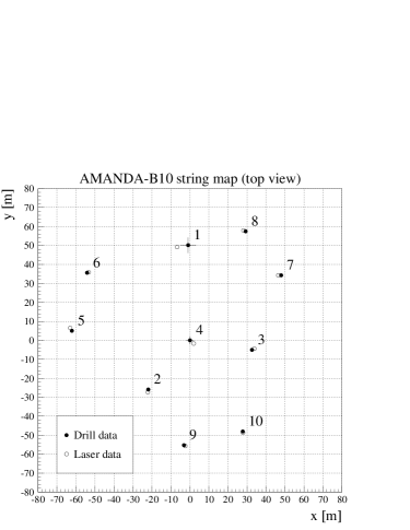
Figure 2: Top view of AMANDA-B10. Open circles denote the positions determined by the laser system, closed circles denote positions obtained from drilling information.

Fig.3 shows data on the wavelength dependence of scattering and absorption compared to theory of He and Price ^?). The absorption length $1/a$ is between 90 and 100 m for wavelengths below 460 nm, i.e. ice absorbs not only about half as much as ocean water, but also does not degrade in transparency towards smaller wavelengths down to 337 nm. On the other hand, scattering is nearly an order of magnitude stronger than in water: the effective scattering length $1/b=$ geometric scattering length/$(1-\langle\cos{\theta}\rangle)$ varies between 24 and 30 m in the relevant wavelength range. $\langle\cos\theta\rangle$ is the average cosine of the scattering angle and is supposed to be about 0.8 in deep ice. These values vary with depth by $\pm 30\%$ between 1.5 and 2.0 km ^?).

Figure 3: Absorption and scattering coefficients at an average depth of 1.7 km.

2 Reconstruction of Muon Tracks

The reconstruction procedure for a muon track consists of five steps:

1. Rejection of noise hits.

2. A line approximation ^?) which yields a first track estimate and a velocity $\vec{v}$.

3. A likelihood fit based on the measured times. This ”time fit” yields angles and coordinates of the track as well as a likelihood ${\cal L}_{time}$.

4. A likelihood fit using the fitted track parameters from the time fit and varying the light emission per unit length until the probabilities of the hit PMTs to be hit and non-hit PMTs to be not hit are maximized. This fit does not vary the direction of the track but yields a likelihood ${\cal L}_{hit}$ with can be used as a quality parameter.

5. A quality analysis applying cuts in order to reject badly reconstructed events.

2.1 Time Fit

In an ideal medium without scattering, one would reconstruct the path of minimum ionizing muons most efficiently by a $\chi^{2}$ minimization. Because of scattering in ice, the distribution of arrival times of photoelectrons seen by a PMT is not Gaussian but has a long tail at the high side – see fig. 4. In order to cope with the non-Gaussian timing distributions we used a likelihood analysis. In this approach, a normalized probability distribution function $p_{i}(t)$ gives the probability of a certain time delay $t$ for a given hit $i$ with respect to straightly propagating photons. This probability function is derived from MC simulations of photon propagation in ice. By varying the track parameters the logarithm of a likelihood function ${\cal L}$ is maximized.

$$\log({\cal L})=\log\left(\prod_{\mbox{all hits}}p_{i}\right)=\sum_{\mbox{all hits}}\log(p_{i})$$

In order to be used in the iteration process, the time delays as obtained from the photon propagation Monte-Carlo have to be parameterized by an analytic formula. The AMANDA collaboration has developed two independent reconstruction programs, using different parameterizations of the photon propagation as well as different minimization methods ^?,?). Both methods are in good agreement with each other. Fig. 4 shows the result of the parameterization of the time delay for two distances and for two angles between the PMT axis and the muon direction.

Figure 4: Arrival time distributions for modules facing (full curves) and back-facing (dashed curves) a muon track. Parameterizations ^?) are shown for muon tracks with impact parameters of 5 meters (a) and 150 meters (b).

At a distance of 5 m and a PMT facing toward the muon track, the delay curve is dominated by the time jitter of the PMT. If the PMT looks into the opposite direction, the contribution of scattered photons yields a long tail towards large delays. At distances as large as 150 m, distributions for both directions of the PMT are close to each other since all photons reaching the PMT are multiply scattered.

2.2 Quality Analysis

Quality criteria are applied in order to select events which are ”well” reconstructed. The criteria define cuts on topological event parameters and observables derived from the reconstruction, e.g.

• Speed $|\vec{v}|$ of the line approximation. Values close to the speed of light indicate a reasonable pattern of the measured times.

• ”Time” likelihood per hit PMT $\log({\cal L}_{time})/N_{hit}$.

• ”Hit” likelihood per all working channels, $\log({\cal L}_{hit})/N_{all}$.

• Number of direct hits, $N_{dir}$, which is defined to be the number of hits with time residuals $t_{i}\mbox{(measured)}-t_{i}\mbox{(fit)}$ smaller than a certain cut value. We use cut values of 15 nsec, 25 nsec and 75 nsec, and denote the corresponding parameters as $N_{dir}$(15), $N_{dir}$(25) and $N_{dir}$(75), respectively. Events with more than a certain minimum number of direct hits (i.e. only slightly delayed photons) are likely to be well reconstructed ^?).

• The projected length of direct hits onto the reconstructed track, $L_{dir}$. A cut in this parameter rejects events with a small lever arm.

• Vertical coordinate of the center of gravity, $z_{COG}$. Cuts on this parameter are used to reject events close to the borders of the array.

3 Verification of reconstruction results by SPASE coincidences

AMANDA is unique in that it can be calibrated by muons with known zenith and azimuth angles which are tagged by air shower detectors at the surface. AMANDA-B4 has been running in coincidence with the two SPASE (South Pole Air Shower Experiment) arrays, SPASE-1 and SPASE-2 ^?) and the GASP Air Cherenkov Telescope. SPASE-2 is located 370 m away from the center of AMANDA. It consists of 30 scintillator stations on a 30 m triangular grid, with a total area of $1.6\cdot 10^{4}$ m². For each air shower, the direction, core location, shower size and GPS time are determined.

A one-week sample of SPASE-2–AMANDA coincidences has been analyzed in order to compare the directions of muons determined by AMANDA-B4 to those of the showers measured by SPASE-2. A histogram of the zenith mismatch angle between SPASE-2 and AMANDA-B4 is shown in fig.5. The selected events are required to have $\geq$8 hits along 3 strings and to yield a track which is closer than 150 m to the air shower axis measured by SPASE-2 (upper histogram). The hatched histogram shows the distribution of the zenith mismatch angle after requesting $\log({\cal L}_{time})/N_{hit}>$ -12, $N_{dir}\mbox{(75)}>4$ and $L_{dir}\mbox{(75)}>50$ m.

428 of the originally 840 selected events pass these quality cuts. The gaussian fit has a mean of $(0.14\pm 0.19)$ degrees and a width of $\sigma=(3.6\pm 0.17)$ degrees. The small mean implies that there is little systematic error in zenith angle reconstruction. The SPASE-2 pointing accuracy depends on zenith angle and shower size and is typically between 1^∘ and 2^{∘ ?)}.

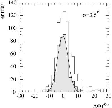
Figure 5: Mismatch between zenith angles determined in AMANDA-B4 and SPASE-2.

4 Results from AMANDA-B4

4.1 Intensity-vs-Depth Relation for Atmospheric Muons

The muon intensity $I(\theta_{\mu})$ as a function of the zenith angle $\theta$ is obtained from

$$I(\theta_{\mu})=\frac{S_{dead}}{T\cdot\Delta\Omega}\,\frac{N_{\mu}(\theta_{\mu})\,\cdot m(\theta_{\mu})}{{\epsilon_{rec}(\theta_{\mu})}\cdot{A_{eff}}(\mbox{cut},\theta_{\mu})}$$ (1)

$N_{\mu}(\theta_{\mu}$) is the number of events with a reconstructed zenith angle $\cos(\theta_{\mu})$. $T=22.03$ hours is the data time used for the atmospheric muon analysis. $S_{dead}$=1.14 accounts for the deadtime of the data acquisition. $\Delta\Omega$ is the solid angle covered by the corresponding $\cos(\theta_{\mu})$ interval. $A_{eff}(\mbox{cut},\theta_{\mu})$ is the effective area at zenith angle $\theta_{\mu}$. The reconstruction efficiency $\epsilon_{rec}(\theta_{\mu})$ is typically 0.8. The mean muon multiplicity $m(\theta_{\mu})$ is about 1.2 for vertical tracks and decreases towards the horizon.

Without applying quality criteria, the zenith angle distribution of the reconstructed muons is strongly smeared. Therefore we have calculated the elements of the parent angular distribution $N_{\mu}(\theta_{\mu})$ from the reconstructed distribution $N_{\mu}(\theta_{rec})$ using a standard regularized deconvolution procedure ^?). The flux $I(\theta)$ can be transformed into a vertical flux $I(\theta=0,h)$, where $h$ is the ice thickness in mwe (meter water equivalent) seen under angle $\theta$:

$$I(\theta=0,h)=I(\theta)\cdot\cos{\theta}\cdot c_{corr}$$ (2)

The $\cos{\theta}$-conversion corrects the sec $\theta$ behaviour of the muon flux, valid for angles up to 60^o. The term $c_{corr}$ is taken from ^?) and corrects for larger angles. It varies between 0.8 and 1.0 for the angular and energy ranges considered here. The vertical intensities obtained in this way are plotted in fig.6. The results are in agreement with the depth-intensity published by DUMAND ^?), Baikal ^?), and the prediction given by Bugaev et al. ^?).

Figure 6: Vertical intensity versus depth for Amanda, Baikal and Dumand. The full line gives the prediction of ^?).

4.2 Search for Upward Going Muons

AMANDA-B4 was not intended to be a full-fledged neutrino detector, but instead a device which demonstrates the feasibiliy of muon track reconstruction in Antarctic ice. The limited number of optical modules and the small lever arms in all but the vertical direction complicate the rejection of fake events. In this section we demonstrate that in spite of that the separation of a few upward muon candidates was possible.

Two full, but independent analysis were performed with the experimental data set of 1996. In the first analysis, a fast pre-filter reduced the background Monte Carlo sample to 5%, whereas 50% of simulated upgoing events survived ^?). Full reconstruction and application of the criteria

1. Hits on $\geq$ 2 strings

2. Reconstructed zenith angle $\theta>$ 90^o

3. $\log({\cal L}_{time})/N_{hit}>-6$

4. $\vec{v_{z}}\geq$ 0.15 m/nsec

5. $N_{dir}(15)\geq$6

reduces the experimental sample to 2 events, in agreement with the Monte Carlo expectation of 2.8 for atmospheric neutrinos. The two events are shown in fig.7.

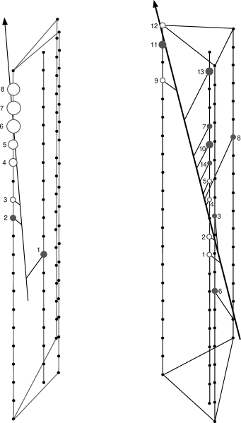
Figure 7: The two experimental events reconstructed as upward muons. left: ID 8427907, right: ID 4706870. The line with an arrow symbolizes the fitted muon track, the lines from this track to the OMs indicates light pathes. The amplitudes are proportional to the size of the OMs. The numbering of the OMs refers to the time order in which they are hit.

For the second analysis, all events have been reconstructed, with different, independent likelihood parametrization and minimisation programs, and then reduced by the subsequent application of the following criteria:

1. zenith angle of the line approximation and of the reconstruction $\theta>120^{o}$,

2. speed of the line approximation $0.15<|\vec{v}|<1$ m/nsec,

3. $\log({\cal L}_{time})/(N_{hit}-5)>-10$,

4. ${\cal L}_{hit}/(N_{hit}-5)>-8$,

5. $N_{dir}(25)\geq 5$,

6. $N_{dir}(75)\geq 9$,

7. $L_{dir}(25)>200$ m,

8. $|z_{COG}|<90$m (absolute value of the vertical coordinate of the center of gravity given by hit OMs).

These cuts reduced the experimental data sample to 3 events. The passing rate for Monte Carlo upward moving muons from atmospheric neutrinos is 1.3%, giving an expectation of 4 events. Two of the three experimental events were also identified in the previously described search, one, however, did not pass the the cut on direct hits ($N_{dir}$=5 instead of 6).

In order to check how well the parameter distributions of the events agree with what one expects for atmospheric neutrino interactions, and how well they are separated from the rest of the experimental data, we relaxed two cuts at a time (retaining the rest) and inspected the distribution in the two ”free” variables.

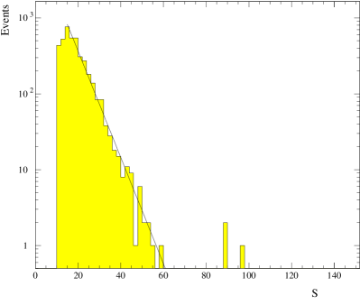
Figure 8: After application of cuts with the exception of cuts 6 and 7: left – distribution in parameters $L_{dir}$(25) vs. $N_{dir}$(75), right: distribution in the ”combined” parameter ($(N_{dir}$(75)-2) $\cdot$ $L_{dir}$(25)/20 m.)

Fig. 8 shows, as an example, the distribution in $L_{dir}$(25) and $N_{dir}$(75). The three events passing all cuts are separated from the bulk of the data. At the bottom of fig. 8, the data are plotted versus a combined parameter, $S=(N_{dir}$(75)-2) $\cdot L_{dir}$(25)/20. In this parameter, the data exhibit a nearly exponential decrease. Assuming the decrease of the background dominated events to continue at higher $S$ values, one can calculate the probability that the separated events are fake events. The probability to observe one event at $S\geq 70$ is 15%, the probability to observe 3 events is only $6\cdot 10^{-4}$.

We conclude that tracks reconstructed as up-going are found at a rate consistent with that expected for atmospheric neutrinos. The three events found in the second analysis are well separated from background. In a limited angular interval, even with a detector as small as AMANDA-B4, neutrino candidates can be separated.

5 Preliminary results from AMANDA-B10

5.1 Separation of atmospheric neutrino events

We have performed a first analysis of data taken during a period of 113 days of the first year of operation (1997) of AMANDA-B10 ^?,?). The corresponding effective live time of the detector is about 85 days. The total experimental sample consists of $4.9\cdot 10^{8}$ events. The events were filtered and reconstructed. After that, a set of quality/upward-muon criteria has been applied. In this first approach, cuts have been applied only to a subset of the parameters used for the B4 analysis. The cuts were grouped into four levels of subsequently increasing tightness. 17 events passed all four cuts, compared to 21.1 events predicted by Monte Carlo. Fig.9 shows the distribution in $\cos\theta$ after cut 2, 3 and 4, respectively. We note that a fine-tuned analysis is expected to yield 2-3 times more events!

Figure 9: Left: The reconstructed zenith angles of 113 days of AMANDA-B10 data after quality cut levels 2 to 4 (from top to bottom). Right: Zenith angle distribution of neutrino candidates (solid line) and of Monte Carlo simulated atmospheric neutrino events normalized to 85 days effective live time (dotted line) at cut level 4.

The 17 upward muon candidates are seen on the left side (the tail of a few additional events on the right side appears since the angular cut were at 80 degrees instead of 90 degrees). Fig.10 shows the zenith angle distribution of the 17 neutrino candidates and of Monte Carlo simulated atmospheric neutrinos. Within the limited statistics, one observes satisfying agreement. Fig.10 displays one neutrino event. Compared to fig.7, it illustrates the significant gain in complexity and information obtained by moving from 4 strings to the 10-string array.

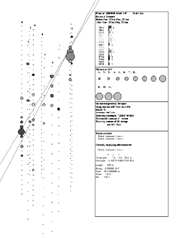
Figure 10: An upgoing muon candidate in Amanda-B10, with 32 hits on 9 strings. The amplitudes are proportional to the diameter of the full circles. In a colored view, their color indicates the time relative to the trigger time. The 2 lines show results of line approximation and final fit.

5.2 Search for relativistic magnetic monopoles

Magnetic monopoles with unit magnetic Dirac charge $g=137/2\cdot e$ and velocities above the Cherenkov threshold in water ($\beta>0.75$) would emit a huge amount of light. Its Cherenkov radiation exceeds that of a bare relativistic muon by a factor $(g\cdot n/e)^{2}=8300$, with $n$=1.33 being the index of refraction for water ^?,?). We therefore searched for events with high hit multiplicity ^?). We analyzed 45 days of effective live time of the 1997 B10 data, yielding $1.8\cdot 10^{6}$ events with mulitplicity larger than 75. In order not to be dominated by brems-showers along downward muons, we applied cuts on the zenith angle $\Theta$ given by the line fit. Obscure time patterns where rejected by cuts on the fitted velocity $v$. To reject high multiplicity events due to cross talk along the cables, special cuts on time differences of hits along one string have been applied.

Monopoles with velocities $\beta$ =0.8, 0.9 and 1.0 have been simulated and tracked through the detector. Fig.11 shows the multiplicity of experimental events after application of all cleaning criteria (left) and that of simulated magnetic monopoles of different velocity after the same criteria. The arrow indicates a cut at multiplicity 120 (clearly above the maximum of 100 hits observed).

Figure 11: Hit multiplicity of events after application of cuts (see text). Left: experimental data. Right: distributions for monopoles with $\beta$= 1.0, 0.9, 0.8 (from top to bottom). The arrow indicates the final multiplicity cut.

With the acceptance for monopoles after all cuts, including the $N_{hit}>120$ cut, being 20.5 (16.0, 9.8)$\cdot 10^{9}$cm²sr for $\beta$ = 1.0 (0.9,0.8), and no experimental event with $N_{hit}>100$, the limit shown in fig.12 is obtained. This limit applies to monopoles with masses larger than $10^{10}-10^{11}$ GeV since lighter monpoles would have been stopped in the Earth.

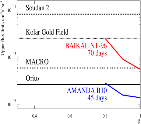
Figure 12: Upper flux limit (90%C.L. for various experiments)

5.3 Other directions of analysis

Results on atmospheric neutrinos and on magnetic monopoles are just examples for a broad front of analyses underway. We mention the following, most of them being reported in contributions to the 26th ICRC:

• Search for point sources of neutrinos. With an area of a few $10^{3}$ m² for TeV neutrinos, AMANDA-B10 is the most sensitive high energy neutrino telescope^?).

• Search for an excess of events over atmospheric neutrinos due to WIMP annihilation in the center of the Earth ^?).

• Search for high energy cascades, similar to our early analysis of AMANDA-A data ^?) and in analogy to the Baikal analysis presented at this Workshop ^?).

• Search for neutrino events in coincidence with GRB coincidences. Since only short time windows bracketing the GRB are scanned, the background rejection criteria can be loosened considerably, resulting in a much higher effective area than in the standard point search analysis ^?).

• Search for counting rate excesses due to a supernova explosion ^?). A future alert algorithm will enable AMANDA to contribute to a worldwide alert network.

• Investigation of seasonal variations of trigger rates which are closely correlated to temperature and pressure of the atmosphere above the South Pole ^?).

6 Future development

In the season 1999/2000, we plan to deploy six additional strings which complete the 30,000 m² telescope AMANDA-II. The new strings will also be used to test a variety of new techniques. Part of the OMs will contain $10^{\prime\prime}$ PMTs with about 50% better light collection. Possibly, wavelength shifters will be applied, which increase the sensitivity in the UV and might give another factor of 30-40% in light collection. The analog transmission of optical signals will be improved, making use of better electronics schemes and of laser diodes instead of LEDs. Another part of the R&D effort is the construction and deployment of a string equipped with digital optical modules in order to investigate waveform digitization at depth ^?). This waveform is then transmitted via a serial link to the surface. The method is challenging since all OMs have to be synchronized on a nanosecond time scale and a complicated communication has to be performed over 2 km electrical cable..

The long-term goal of the collaboration is a detector of the scale of a cube kilometer^?). This is the order of magnitude suggested by many models of neutrino production in AGN, in the center of the Galaxy, in the center of the Earth (due to WIMP annihilation) and in young supernovae ^?). A straw-man design calls for a total of about 5000 PMTs at 80 strings, horizontally spaced by 80-100 meters. The strings would be instrumented between 1.4 and 2.4 km. The approximate cost for the detector can be derived from the estimated cost of 6-8 k$ per channel (including cables and electronics), and amounts to about 35 M$. Construction of ICECUBE will be staged over five to six deployments (possibly 2002/03 to 2007/08.)

7 Acknowledgments

This research was supported by the U.S. National Science Foundation, Office of Polar Programs and Physics Division, the University of Wisconsin Alumni Research Foundation, the U.S. Department of Energy, the U.S. National Energy Research Scientific Computing Center, the Swedish Natural Science Research Council, the Swedish Polar Research Secretariat, the Knut and Alice Wallenberg Foundation, Sweden, and the Federal Ministery for Education and Research, Germany.

References

- [1] D.M.Lowder et al., Nature 353 (1991) 331.
- [2] E.Andres et al., paper submitted to Astroparticle Physics.
- [3] K.Woschnagg et al., paper HE 4.1.15 submitted to the 26th ICRC, Salt Lake City, USA (1999).
- [4] Y.He and B.Price, Geophys. Res. Lett.25 (1998) 2845.
- [5] R.Porrata et al., Proc. 25th ICRC, Durban, South Africa, 7 (1997) 237.
- [6] see the talk of Zh.Djilkibaev, these proceedings.
- [7] V.J.Stenger, preprint HDC-1-90, Hawaii 1990.
- [8] A.Bouchta, PhD thesis, Stockholm 1998, USIP Report 98-07.
- [9] C.Wiebusch et.al., Proc. 25th ICRC, Durban, South Africa, 7 (1997) 13.
- [10] J.Dickinson et al., Proc. 25th ICRC, Durban, South Africa, 5 (1997) 233.
- [11] T.K.Gaisser et al., Proc. 24th ICRC, Rome, Italy, 1 (1995) 938.
- [12] S.Hundertmark, PhD thesis, Zeuthen 1998, and paper HE 3.1.06 submitted to the 26th ICRC, Salt Lake City, USA (1999).
- [13] V.Blobel, DESY84-118, 1984.
- [14] J.Babson et al., Phys.Rev. D42 (1990) 41.
- [15] I.A.Belolaptikov et al., Astropart.Physics 7 (1997) 263.
- [16] E.Bugaev et al., Phys.Rev. D58 (1998).
- [17] P.Lipari, Astropart.Phys. 1 (1993) 1995.
- [18] J.L.Thorn et al., Phys.Rev. D46 (1992) 4846.
- [19] V.A.Balkanov et al., paper HE 5.3.04 submitted to the 26th ICRC, Salt Lake City, USA (1999).
- [20] T.Gaisser, F.Halzen, T.Stanev, Physics Report 258 (1995) 174.
- [21] A. Karle for the Amanda collaboration, paper HE 4.2.05 submitted to the 26th ICRC, Salt Lake City, USA (1999).
- [22] G.Hill for the Amanda collaboration, ibid. HE 6.3.02.
- [23] P.Niessen for the AMANDA collaboration, ibid. HE 5.3.06.
- [24] J.Kim for the Amanda collaboration, ibid. HE 4.2.14.
- [25] E.Dalberg for the Amanda collaboration, ibid. HE 5.3.06.
- [26] R.Bay for the Amanda collaboration, ibid. HE 4.2.06.
- [27] R.Wischnewski for the Amanda collaboration, ibid. HE 4.2.07.
- [28] A.Bouchta for the Amanda collaboration, ibid. HE 3.2.11.
- [29] D.Lowder et al., ibid. HE 6.3.07.
- [30] F.Halzen for the Amanda collaboration, ibid. HE 6.3.01.