Cosmological evolution and hierarchical galaxy formation

Abstract

We calculate the rate at which dark matter halos merge to form higher mass systems. Two complementary derivations using Press-Schechter theory are given, both of which result in the same equation for the formation rate. First, a derivation using the properties of the Brownian random walks within the framework of Press-Schechter theory is presented. We then use Bayes’ theorem to obtain the same result from the standard Press-Schechter mass function. The rate obtained is shown to be in good agreement with results from Monte-Carlo and N-body simulations. We illustrate the usefulness of this formula by calculating the expected cosmological evolution in the rate of star formation that is due to short-lived, merger-induced starbursts. The calculated evolution is well-matched to the observed evolution in ultraviolet luminosity density, in contrast to the lower rates of evolution that are derived from semi-analytic models that do not include a dominant contribution from starbursts. Hence we suggest that the bulk of the observed ultraviolet starlight at $z>1$ arises from short-lived, merger-induced starbursts. Finally, we show that a simple merging-halo model can also account for the bulk of the observed evolution in the comoving quasar space density.

1 Introduction

If the matter content of the universe is dominated by cold dark matter, then dark matter halos associated with galaxies are expected to form hierarchically. Bond et al. [Bond et al. 1991] have shown that a more rigorous treatment of the work of Press & Schechter [Press & Schechter 1974] can be used to obtain information about the build-up of structure. Calculations using Press-Schechter (PS) theory are based on a statistical analysis of the initial field of density perturbations and do not include any non-linear dynamical effects, but nonetheless the results appear to agree well with dynamical, collisionless (“N-body”) simulations [Lacey & Cole 1994, Somerville et al. 1998].

The aim of this paper is to use PS theory to calculate the rate of formation of dark halos of specified mass. We compare the results with those of Monte-Carlo and N-body simulations, and we also use the calculations to argue that the bulk of the observed cosmological evolution in star-formation and quasar activity is a reflection of the evolution in rate of dark halo formation.

A standard application of PS theory is to calculate the mass function given a cosmic epoch of interest. In many cosmological situations we are also interested in the rate at which halos of some mass form. Consequently, there have been a number of attempts to estimate this rate using PS theory [Lacey & Cole 1993, Sasaki 1994]. In this paper we use the theory of random walks within the PS framework to calculate directly the halo formation rate for any cosmology. We also use Bayes’ theorem to derive the same equation from the standard PS mass function. These complementary methods provide important insights into how the formation of halos can be understood within PS theory.

In section 5 we use a Monte-Carlo realisation of actual Brownian random walks to calculate the formation epochs of the halos they represent. The distribution of these epochs is found to be in good agreement with the formula calculated previously. Following this we show that the formation time distribution of halos in a large N-body simulation (found using a standard friend-of-friends algorithm) is also well approximated by the PS result.

We then discuss the relevance of this work to our understanding of the observed cosmological evolution in star-formation rate (SFR) and quasar space density. In particular we suppose that there is a causal link between the hierarchical formation of dark halos and the activation of both quasars and luminous bursts of star formation. The possibility of a connection between these two key evolving quantities has already been suggested by a number of authors [Shaver et al. 1996, Dunlop 1997, Boyle & Terlevich 1998]. Mergers and interactions have long been implicated in both luminous starbursts and active galaxies (see the review by Barnes & Hernquist 1992 and refs therein) and merging galaxies have been found in which both phenomena are observed [Canalizo & Stockton 1997, Stockton, Canalizo & Close 1998, Brotherton et al 1999]. Investigation of the galaxies found at redshifts around 3 by the Lyman-break method [Steidel et al. 1998a] show that much of the ultraviolet light inferred to be due to star formation can be identified with individual galaxies with star formation rates of possibly up to $1000{\rm\,M_{\odot}}$ per year [Steidel et al. 1998b]. These galaxies are strongly clustered and hence are likely to be the progenitors of cluster galaxies at the present epoch (Steidel et al. 1998a,b; Adelberger et al. 1998): at high redshifts there is therefore direct evidence for a link between the high level of star formation and host galaxies which are inferred to be merging into higher-mass galaxy systems. The detailed physics of both quasar- and star-formation is complicated and not understood, and in this paper we discuss only the role that the cosmological variation in halo formation rate might have in determining the evolution in observed quantities such as the ultraviolet luminosity density arising from star formation.

2 Press-Schechter theory

We now describe briefly the principles of Press-Schechter (PS) theory and calculate the number density of halos at a particular epoch - the standard PS formula; a result which has been shown to be in good agreement with N-body simulations (e.g. Efstathiou et al. 1988).

Dark halos are assumed to form by the non-linear gravitational collapse of initial density perturbations. We assume that the initial perturbations form a homogeneous, isotropic Gaussian random field. In PS theory such a field is smoothed by convolving with a filter function whose size is related to the mass $M$ of halo in which we are interested. The fractional overdensity at any location is assumed to grow linearly until a critical overdensity, $\delta_{c}$, is reached, when that location is considered to have collapsed into a dark halo of mass $M$, provided that the critical overdensity is not exceeded when the field is filtered on a scale corresponding to a larger mass. In the analysis that follows, instead of viewing the field as growing with time, we consider the field to be fixed and the critical overdensity $\delta_{c}$ to decrease with time.

If we use a sharp k-space filter of radius R, $W(\mathbf{r};R)=(\sin(r/R)-(r/R)\cos(r/R))/(r/R)^{3}$, the density of the filtered field at any point is given by a Brownian random walk with the variance of the filtered field being the ‘time’ axis [Peacock & Heavens 1990, Bond et al. 1991]. The mass associated with this point in space is given by the position of the first upcrossing of an absorbing barrier at $\delta=\delta_{c}(t)$. The probability density function that a trajectory will have its first upcrossing at a mass between $M$ and $M+dM$, $P(M|\delta_{c})dM$ is given by a solution of the diffusion equation with an absorbing boundary condition [Bond et al. 1991]:

$$P(M|\delta_{c})dM=\frac{\delta_{c}}{(2\pi)^{1/2}\sigma_{M}^{3}}\exp\left(-\frac{\delta_{c}^{2}}{2\sigma_{M}^{2}}\right)\left|\frac{d\sigma_{M}^{2}}{dM}\right|dM$$ (1)

where $\sigma_{M}^{2}$ is the variance of the filtered field which for a sharp k-space filter is given by:

$$\sigma_{M}^{2}=\frac{1}{2\pi^{2}}\int_{0}^{2/R}k^{2}P(k)dk$$ (2)

where $P(k)$ is the power spectrum of the initial random field. We can use equation 1 to obtain the comoving number density of halos of mass M at a given time t, $n(M|t)$:

$$n(M|t)MdM=\rho P(M|\delta_{c}(t))dM$$

$$\hskip 28.45274pt=2\rho\frac{\delta_{c}(t)}{(2\pi)^{1/2}\sigma_{M}^{2}}\exp\left(-\frac{\delta_{c}(t)^{2}}{2\sigma_{M}^{2}}\right)\left|\frac{d\sigma_{M}}{dM}\right|dM.$$ (3)

This is the standard PS mass function. It should be noted that when using other filters this result is not correct [Bond et al. 1991, Jedamsik 1995, Yano, Nagashima & Gouda 1996].

To calculate the numbers of halos and their rate of formation we need to normalise the power spectrum. We require the variance in the density field when filtered with a top-hat filter of radius $8h^{-1}$ Mpc, $\sigma_{8}$, to match the values deduced from X-ray clusters [Eke, Cole & Frenk 1996].

For a top-hat filter, we can relate the mass of a halo to the filter radius, $M=4/3\pi{\rho}R^{3}$. We can also calculate the critical overdensity for collapse for a uniform spherical region; for a flat $\Omega_{\Lambda}=0$ universe this is given by $\delta_{c}=\alpha(1+z)$, where $\alpha\sim 1.68$ [Gunn & Gott 1972]. For an open $\Omega_{\Lambda}=0$ universe, $\delta_{c}(z)$ is given by Lacey & Cole [Lacey & Cole 1993], and for a flat $\Omega_{\Lambda}\neq 0$ universe by Eke, Cole & Frenk [Eke, Cole & Frenk 1996]. For a sharp k-space filter, the relationship between the mass and filter size is less obvious. Following Lacey and Cole [Lacey & Cole 1993], we integrate the filter function over all space to obtain its ‘volume of influence’, which gives $M=3/4\pi^{2}\rho R^{3}$. However, if we use the critical overdensity applicable to the top-hat filter used to normalise the power spectrum the k-space filter predicts a different number density of halos. We therefore choose the critical overdensity associated with a sharp k-space filter to be that which predicts the same number density of halos for both filters at the mass used to normalise the power spectrum.

3 Derivation of the halo formation rate from PS theory

We now use PS theory to obtain more information about the build-up of structure, in particular to calculate the rate at which dark halos of a particular mass form. We cannot calculate this simply by taking the time derivative of equation 3 as, in PS theory, halos are not only being continually formed at any particular mass but are also continually being lost into halos of higher mass. We present new work to calculate the required halo formation rate by examining properties of the Brownian random walks invoked in standard PS theory. We use the fact that the rate of halo formation is equivalent to a probability density function in time. The analysis of Brownian random walks is important in many fields of pure and applied science and similar results to those derived below can also be found in many introductory books on stochastic processes (e.g. Karlin & Taylor 1975).

Initially, suppose that we are not interested in how the halo formed so we are not interested in the shape of the trajectory up until the epoch of halo formation. We wish to calculate the distribution of cosmic epochs at which halos of a given mass $M$ are first formed, $P(t|M)$dt. In PS theory, this probability density function is related by a variable transformation to $P(\delta_{c}|\sigma_{M}^{2})$, the probability that a trajectory has its first upcrossing between $\delta_{c}$ and $\delta_{c}+d\delta_{c}$ at a given value of $\sigma_{M}^{2}$, and it is a formula for this that we now derive using the trajectories approach. We let $\delta(\sigma_{M}^{2})$ be the position of the walk at $\sigma_{M}^{2}$ and define:

$$\delta_{\rm max}(\sigma_{M}^{2})=\mbox{\rm max}\{\delta(\sigma_{M^{\prime}}^{2});0\leq\sigma_{M^{\prime}}^{2}\leq\sigma_{M}^{2}\},$$ (4)

$$\delta_{\rm diff}(\sigma_{M}^{2})=\delta_{\rm max}(\sigma_{M}^{2})-\delta(\sigma_{M}^{2}).$$ (5)

Figure 2: The solid line represents a random walk consisting of 70 equally spaced steps of $\sigma_{M}^{2}$ in the interval $0<\sigma_{M}^{2}<1.4$. The random walk was chosen from a set of such walks and is such that $\delta_{\rm max}(1.4)>m$ and $\delta(1.4)<x$. The dotted line represents the walk obtained by reflecting the initial trajectory about the line $\delta=m$ after the first upcrossing of this line. Note that it has the property that $\delta(1.4)>2m-x$. Similarly, any trajectory which is such that $\delta(1.4)>2m-x$ can undergo a similar reflection to obtain a trajectory with $\delta_{\rm max}(1.4)>m$ and $\delta(1.4)<x$. There is a one-to-one correspondence between walks with $\delta_{\rm max}(\sigma_{M}^{2})>m$ and $\delta(\sigma_{M}^{2})<x$ and walks with $\delta(\sigma_{M}^{2})>2m-x$.

By considering the reflection of trajectories about the line $\delta=m$ beyond the first upcrossing of this line, we can see that there is a one-to-one correspondence between trajectories for which $\delta(\sigma_{M}^{2})>2m-x$ and trajectories for which $\delta_{\rm max}(\sigma_{M}^{2})>m$ and $\delta(\sigma_{M}^{2})<x$ where $x<m$. For a pictorial representation of this correspondence see Fig. 2. This means that:

$$P(\delta_{\rm max}(\sigma_{M}^{2})\geq m,\delta(\sigma_{M}^{2})\leq x|\sigma_{M}^{2})$$

$$\hskip 28.45274pt=P(\delta(\sigma_{M}^{2})\geq 2m-x|\sigma_{M}^{2})$$

$$\hskip 28.45274pt=\frac{1}{2}\left[1-\mbox{erf}\left(\frac{2m-x}{(2\sigma_{M}^{2})^{1/2}}\right)\right],m\geq 0,m\geq x.$$ (6)

We differentiate with respect to x and then with respect to m, changing the sign, to get the joint density function for $\delta_{\rm max}(\sigma_{M}^{2})$ lying in the interval $m,m+dm$ and $\delta(\sigma_{M}^{2})$ lying in the interval $x,x+dx$. This gives:

$$f(m,x|\sigma_{M}^{2})dmdx$$

$$\hskip 28.45274pt=\sqrt{\frac{2}{\pi}}\frac{2m-x}{(\sigma_{M}^{2})^{3/2}}\exp\left(\frac{-(2m-x)^{2}}{2\sigma_{M}^{2}}\right)dmdx,$$ (7)

$$\hskip 28.45274pt0\leq m,x\leq m.$$

To obtain the joint density function for $\delta_{\rm max}(\sigma_{M}^{2})$ lying in the interval $m,m+dm$ and $\delta_{\rm diff}(\sigma_{M}^{2})$ lying in the interval $y,y+dy$ we note that:

$$P(\delta_{\rm max}(\sigma_{M}^{2})\leq a,\delta_{\rm diff}(\sigma_{M}^{2})\leq b|\sigma_{M}^{2})$$

$$\hskip 28.45274pt=\int_{0}^{a}\int_{0}^{b}f(m,m-y)dydm.$$ (8)

From this we can deduce that the desired joint density is g(m,y)=f(m,m-y):

$$g(m,y|\sigma_{M}^{2})dmdy$$

$$\hskip 28.45274pt=\sqrt{\frac{2}{\pi}}\frac{m+y}{(\sigma_{M}^{2})^{3/2}}\exp\left(\frac{-(m+y)^{2}}{2\sigma_{M}^{2}}\right)dmdy,$$ (9)

$$\hskip 28.45274ptm\geq 0,y\geq 0.$$

We now calculate $g(m|y=0,\sigma_{M}^{2})$ using Bayes’ theorem to transform from equation 9 to the conditional probability required and then setting $y=0$. This is equivalent to setting $y=0$ in equation 9 and renormalising so the probability density function integrates to 1. Integrating $g(m,y|\sigma_{M}^{2})dmdy$ we see that:

$$g(y|\sigma_{M}^{2})dy=\sqrt{\frac{2}{\pi}}\frac{1}{(\sigma_{M}^{2})^{1/2}}\exp\left(\frac{-y^{2}}{2\sigma_{M}^{2}}\right)dy,y\geq 0,$$ (10)

and applying Bayes’ theorem we find that:

$$g(m|y,\sigma_{M}^{2})=\frac{m+y}{\sigma_{M}^{2}}\exp\left(\frac{-(m+y)^{2}+y^{2}}{2\sigma_{M}^{2}}\right)dm,$$ (11)

$$\hskip 28.45274ptm\geq 0.$$

It just remains to set $y=0$ and change the variable from m to $\delta_{c}$ which we now take to be the position of the first upcrossing:

$$P(\delta_{c}|\sigma_{M}^{2})d\delta_{c}=\frac{\delta_{c}}{\sigma_{M}^{2}}\exp\left(-\frac{\delta_{c}^{2}}{2\sigma_{M}^{2}}\right)d\delta_{c}.$$ (12)

This is the probability that a trajectory has its first upcrossing between $\delta_{c}$ and $\delta_{c}+d\delta_{c}$ at a given value of $\sigma_{M}^{2}$.

By changing the variables from $\sigma_{M}^{2}$ to mass $M$ and from $\delta_{c}$ to time $t$, we obtain the probability that a halo of mass $M$ formed between times $t$ and $t+dt$. This gives the dependence on cosmic epoch of the rate of halo formation:

$$P(t|M)dt=\frac{\delta_{c}}{\sigma_{M}^{2}}\exp\left(-\frac{\delta_{c}^{2}}{2\sigma_{M}^{2}}\right)\left|\frac{d\delta_{c}}{dt}\right|dt.$$ (13)

In the special case of a flat $\Omega_{\Lambda}=0$ cosmology for which $\delta_{c}=\alpha(1+z)$, this time evolution is given by the simple formula:

$$\left(\frac{dn}{dt}\right)^{+}\propto(1+z)^{3.5}\exp(-\beta(1+z)^{2})$$ (14)

where $\beta=\alpha^{2}/(2\sigma_{M}^{2})$ is a function of the mass of halo and the power spectrum.

We note that because the trajectories are Brownian random walks, all walks which pass through a given point can be thought of as new walks starting from that point. It is thus possible to apply coordinate changes to equation 1 and obtain the conditional probability for the mass distribution of progenitors of halos [Bond et al. 1991]. Using Bayes’ theorem and this result it is also possible to calculate the distribution of final collapsed masses attained by halos given the mass at an earlier time [Lacey & Cole 1993].

We can apply a similar argument to the result derived above for the time distribution of formation events and obtain the distribution of times at which a halo formed, given that it formed part of a larger halo at a known later time. If we consider walks starting from ($\sigma_{M^{\prime}}^{2},\delta_{c}^{\prime}$), where $\sigma_{M^{\prime}}^{2}<\sigma_{M}^{2}$ and $\delta_{c}^{\prime}<\delta_{c}$ (i.e. $M^{\prime}>M$ and $t^{\prime}>t$) we obtain the required conditional probability:

$$P(\delta_{c}|\sigma_{M}^{2},\delta_{c}^{\prime},\sigma_{M^{\prime}}^{2})d\delta_{c}$$

$$\hskip 28.45274pt=\frac{\delta_{c}-\delta_{c}^{\prime}}{\sigma_{M}^{2}-\sigma_{M^{\prime}}^{2}}\exp\left(-\frac{(\delta_{c}-\delta_{c}^{\prime})^{2}}{2(\sigma_{M}^{2}-\sigma_{M^{\prime}}^{2})}\right)d\delta_{c}.$$ (15)

The behaviour of a trajectory, having passed through a point related to the formation of a halo, thus provides mass and formation time distributions for the progenitors of the halo. As noted above, the form of the trajectory continuing from such a formation point is independent of the position of that point, and consequently the mass distribution of progenitors immediately prior to the formation event is independent of the formation epoch. Turning this argument around, we see that the effect of placing constraints on the progenitors of the halo immediately prior to the formation event doesn’t affect the distribution of formation times. We thus have the important result that, even if we only consider formation events resulting from mergers with specified progenitors, such as halos resulting from a merger of two approximately equally sized objects, the distribution of times at which these mergers occur is still that given by equation 13. It is for this reason that we consider the cosmic variation in halo formation rate also to be a measure of the cosmic variation in the rate of mergers between dark halos. We should note that because standard PS theory does not account for halo sub-structure, the derivation presented here excludes possible mergers between low-mass halo sub-units forming part of a larger collapsed halo.

4 An alternative derivation

We will now show that $P(t|M)$dt as given by equation 13 can be calculated from the conditional probability density function $P(M|t)$dM [Bond et al. 1991] using Bayes’ theorem. Firstly, we wish to calculate the prior for $\delta_{c}$ which is equivalent to asking the question ‘Given no knowledge of $\sigma_{M}^{2}$, what is the distribution of upcrossing points in $\delta_{c}$?’. We note that all trajectories must have an upcrossing point of any given line $\delta=\delta_{c}$. Now, in any two equally sized intervals, $d\delta_{1}$ and $d\delta_{2}$, there must be equal probability of such a crossing existing because the walk does not alter its form at different $\delta_{c}$ (all walks which pass through a given point can be thought of as new walks starting from that point). Thus, given no a priori information about $\sigma_{M}^{2}$, all values of $\delta_{c}$ are equally likely and we should assume a uniform prior for $\delta_{c}$. In order to be mathematically rigorous, we must make $\delta_{c}$ bounded. We see later that we can remove these bounds without affecting the result. So we have that:

$$P(\delta_{c})d\delta_{c}=\left\{\begin{array}[]{ll}\frac{d\delta_{c}}{\delta_{\rm max}-\delta_{\rm min}}&\mbox{$\delta_{\rm min}\leq\delta_{c}\leq\delta_{\rm max}$}\\ 0&\mbox{otherwise.}\end{array}\right.$$ (16)

Applying Bayes’ theorem and using equation 1, we can find the joint probability of $\delta_{c}$ and $\sigma_{M}^{2}$:

$$P(\sigma_{M}^{2},\delta_{c})d\sigma_{M}^{2}d\delta_{c}=\frac{1}{(\delta_{\rm max}-\delta_{\rm min})}$$

$$\hskip 28.45274pt\times\frac{\delta_{c}}{(2\pi)^{1/2}(\sigma_{M}^{2})^{3/2}}\exp\left(-\frac{\delta_{c}^{2}}{2\sigma_{M}^{2}}\right)d\sigma_{M}^{2}d\delta_{c}.$$ (17)

We can integrate this equation over all $\delta_{c}$ to obtain the probability density function for $\sigma_{M}^{2}$:

$$P(\sigma_{M}^{2})d\sigma_{M}^{2}=\frac{1}{(2\pi)^{1/2}(\sigma_{M}^{2})^{1/2}(\delta_{\rm max}-\delta_{\rm min})}$$

$$\hskip 28.45274pt\times\left[\exp\left(-\frac{\delta_{\rm min}^{2}}{2\sigma_{M}^{2}}\right)-\exp\left(-\frac{\delta_{\rm max}^{2}}{2\sigma_{M}^{2}}\right)\right],$$ (18)

and again use Bayes’ theorem to obtain the conditional probability $P(\delta_{c}|\sigma_{M}^{2})$:

$$P(\delta_{c}|\sigma_{M}^{2})d\delta_{c}=\frac{\delta_{c}}{\sigma_{M}^{2}}\exp\left(-\frac{\delta_{c}^{2}}{2\sigma_{M}^{2}}\right)d\delta_{c}$$

$$\hskip 28.45274pt\times\left[\exp\left(-\frac{\delta_{\rm min}^{2}}{2\sigma_{M}^{2}}\right)-\exp\left(-\frac{\delta_{\rm max}^{2}}{2\sigma_{M}^{2}}\right)\right].$$ (19)

In the limit as $\delta_{\rm min}\rightarrow 0$ and $\delta_{\rm max}\rightarrow\infty$ this becomes:

$$P(\delta_{c}|\sigma_{M}^{2})d\delta_{c}=\frac{\delta_{c}}{\sigma_{M}^{2}}\exp\left(-\frac{\delta_{c}^{2}}{2\sigma_{M}^{2}}\right)d\delta_{c}.$$ (20)

This is the probability that given a particular value of $\sigma_{M}^{2}$, the first upcrossing at this $\sigma_{M}^{2}$ has probability $P(\delta_{c}|\sigma_{M}^{2})$ of being between $\delta_{c}$ and $\delta_{c}+d\delta_{c}$. This probability is identical to that calculated directly from the Brownian random walks in section 3.

5 Comparison with results from Monte-Carlo simulation

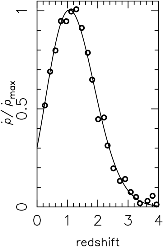
Figure 4: Comparison of Monte-Carlo results with Press-Schechter predictions of the halo formation rate at fixed final mass. Open symbols show Monte-Carlo results of the formation time of a halo of mass $1.3\times 10^{13}{\rm\,M_{\odot}}$ for a standard CDM power spectrum with shape parameter $\Gamma=0.25$ normalised to $\sigma_{8}=0.64$. The solid curve shows the prediction of equation 14 at this mass. The results are normalised to give a peak formation rate of 1.

As a check on the validity of equation 14 we have performed Monte-Carlo simulations to calculate random trajectories and determine the distribution of formation epochs. Approximately $10^{6}$ random walks were constructed, each consisting of $2^{11}$ uniform steps in $\sigma_{M}^{2}$ between 0 and $\sigma_{M}^{2}$ equivalent to a mass of $1.3\times 10^{13}{\rm\,M_{\odot}}$ for a standard CDM power spectrum with shape parameter $\Gamma=0.25$ normalised to $\sigma_{8}=0.64$. Of these walks, $10^{4}$ were recorded with first upcrossing points at the final value of $\sigma_{M}^{2}$. The distribution of these upcrossing points was recorded in uniform bins in time and is compared with the expected distribution given by equation 14 in Fig 4. Good agreement is demonstrated.

6 Comparison with results from N-body simulation

Figure 6: Comparison of N-body results with Press-Schechter predictions of the halo formation rate at fixed final mass. The solid symbols show the N-body results for groups of between 45 and 55 particles, corresponding to a mass of approximately $1.3\times 10^{13}{\rm\,M_{\odot}}$, see text for details. The solid curve shows the prediction of equation 14 at this mass with parameters as given in the text and normalised to the N-body values.

We present results from a simulation run using the Hydra N-body, hydrodynamics code [Couchman, Thomas & Pearce 1995]. The simulation used $128^{3}$ dark matter particles in a flat universe with $\Omega_{M}=1$, $\Omega_{\Lambda}=0$, $h=0.5$, and standard CDM power spectrum with shape parameter $\Gamma=0.25$. The power spectrum was normalised to $\sigma_{8}=0.64$. Groups of particles were found using a standard friends of friends (FOF) algorithm which links two particles together if the mean overdensity of a grid of particles with the same separation is greater than that predicted at the moment of virialisation for spherical top-hat collapse [Peebles 1980].

In order to calculate the rate at which halos form we analysed results from the N-body run at 104 different times, separated by equal intervals of time. By comparing the FOF results at each output time to results from earlier times we were able to build up a picture of the hierarchical growth of structure. Halos with at least half of the component particles not observed in a halo of equal or higher mass at an earlier time were recorded as being formed in the time interval between this output time and the previous one. There is a problem in this analysis that we may miss formation events - a halo formed in the time interval of interest may have already merged into a halo of higher mass when we analysed the simulation. However we can estimate the potential error caused by this effect by calculating the maximum amount of halos which could have been formed from the data on all new halos. The distribution of new halos of between 45 and 55 particles is shown in Fig. 6. The symbols mark the average of the minimum and maximum mass which could have been involved in mergers per unit time. The minimum is just the recorded mass in new halos of between 45 and 55 particles, the maximum is the mass in all new halos of greater than 45 particles which could have passed through the interval of interest. The error bars mark the positions of these maximum and minimum points. Note that these error bars only denote the error in measuring the mass formation rate from the N-body simulation results - they do not include errors intrinsic to the N-body simulation.

In order to count enough formation events we had to use a reasonably large interval in mass, corresponding to between 45 and 55 particles. However, the curve predicted from equation 14 is similar within this mass range, and the error caused by this effect will be small. In Fig. 6 we plot the prediction from equation 14 at a mass equivalent to 50 particles which shows remarkably good agreement with the results of the N-body simulation. Note that we have not renormalised any of the parameters of the PS models other than by the self-consistent method given in section 2. One caveat we should note, however, is that we have only been able to test the agreement between the PS result and N-body simulation at relatively high halo masses.

7 Comparison with previous results

We consider that the formation of a halo occurs when all of the mass in the halo is assembled. Blain & Longair [Blain & Longair 1993] and Sasaki [Sasaki 1994] also used the same definition of ‘formation’, and tried to calculate the rate of halo formation from the standard PS mass function (equation 3) and its derivative. However, they both made assumptions beyond standard PS theory. Blain & Longair [Blain & Longair 1993] calculated the formation rate empirically assuming a form for the distribution of mergers which occur. Sasaki [Sasaki 1994] obtained an equation for the formation rate assuming the destruction rate (from which they then calculate the formation rate) for a power-law spectrum has no characteristic mass scale. These assumptions lead to different forms for the formation rate from that derived above where we have not made any assumptions beyond those of standard PS theory.

Lacey & Cole (1993) defined the formation time as the time when the largest progenitor of a halo first contains at least half the mass of the halo. Using our definition of formation, we see that the distribution of such times is equivalent to the formation time distribution of progenitors of mass greater than M/2 given that they are the first such progenitors for a particular halo. The formation time distribution of progenitors of mass M given by equation 15 is only dependent on knowing that a progenitor of mass M is formed at some epoch. For instance by setting $M=M^{\prime}/2$ in equation 15 we can calculate the distribution of times at which progenitors of mass $M^{\prime}/2$ form, given that a progenitor of mass $M^{\prime}/2$ is formed at some time. However, we do not know that the first subclump has mass $M^{\prime}/2$, only that it lies in the range $M^{\prime}/2<M<M^{\prime}$ - this is a consequence of PS theory containing mass jumps. Lacey & Cole (1993) give a counting argument (their section 2.5.2) which converts from a probability density in mass to a distribution in the number of progenitors in order to set the condition that we are only interested in the first halo to contain at least half the mass of the final halo. Without such an argument it is difficult to see how to distinguish the first progenitor from subsequent ones and so the results of this paper are not directly comparable to those of Lacey & Cole.

model	$\Omega_{M}$	$\Omega_{\Lambda}$	$\Gamma$	$h$	$\sigma_{8}$
OCDM	0.3	0	0.15	0.5	0.85
$\Lambda$CDM	0.3	0.7	0.15	0.5	0.91
SCDM	1	0	0.5	0.5	0.60
$\Gamma$CDM	1	0	0.25	0.5	0.60

Table 2: Table of parameters used for each of the 4 cosmological models chosen. Here $h=H_{0}/100$ km s^-1 Mpc^-1, $\Omega_{M}\equiv\frac{8\pi G}{3H_{0}^{2}}\rho_{M0}$, $\Omega_{\Lambda}\equiv\frac{\Lambda}{3H_{0}^{2}}$, and $\Gamma$ is the CDM power spectrum shape parameter.

8 The predicted halo formation rate

We can now estimate the rate at which mergers occur to create halos of any particular mass for a number of cosmologies. We investigate 4 different cosmologies, based on those used by the Virgo consortium [Springel et al. 1998, Jenkins et al. 1998] summarised in Table 2.

Fig. 8 shows how the functions vary with halo mass for the $\Gamma$CDM model. Curves are plotted at 4 different values of halo mass, $10^{10.5}-10^{12}{\rm\,M_{\odot}}$. Here it is easy to see the hierarchical build up of structure - low mass halos predominantly form first, with their peak formation rate occurring at higher redshift than that for higher mass halos.

Figure 8: The formation rate of galaxy halos as calculated using equation 13 for the $\Gamma$CDM cosmological model. Curves are plotted for halo masses in the range $10^{10.5}-10^{12.0}{\rm\,M_{\odot}}$ and are normalised to give the same peak formation rate.

For each cosmology chosen, for a particular mass of halo, the redshift at which the formation rate peaks is highly dependent on the $\sigma_{8}$ normalisation chosen. High values of $\sigma_{8}$ lead to early formation and the peak in the formation rate is at higher redshift. However by choosing a higher halo mass we can recover the same shape of curve. This is easy to see in the SCDM and $\Gamma$CDM cosmologies, where equation 14 applies, and the curve shape is only dependent on the value of $\beta$ which can be kept constant by varying the halo mass with $\sigma_{8}$. Fig. 10 shows the mass merging rate for each of the cosmological models, but with halo masses chosen such that the models approximately agree on the redshift of the peak of halo formation. Viewed in this way, the OCDM model produces less evolution than the other models, but the other three have rather similar amounts of evolution.

Figure 10: Comparison of the 4 different cosmological models. Because of the differing normalisations of the models the formation rates are plotted for different values of the halo mass, chosen to provide the closest match between the models. The masses are: OCDM, $10^{12.7}{\rm\,M_{\odot}}$; $\Lambda$CDM, $10^{12.0}{\rm\,M_{\odot}}$; SCDM, $10^{12.1}{\rm\,M_{\odot}}$; $\Gamma$CDM, $10^{11.1}{\rm\,M_{\odot}}$. The curves are normalised to the same peak formation rate.

9 The Merger-Induced Star Formation Rate

A complete description of the formation of stars in hierarchically-forming galaxies requires us to understand mergers between dark halos, the fate of the baryonic matter in such mergers, and the processes of cooling, star formation and feedback and stellar evolution that all affect the observed luminosity of a galaxy and its time variation. Some recent attempts to explain specifically the strong evolution in star formation have used ad hoc models of the rate of generation of new galaxies as a source function, which have then been combined with models describing the remaining processes and tested against the observed data in sub-mm, infrared, optical and ultraviolet wavebands (Madau et al. 1996, 1998). An alternative method is to simulate the merger histories of galaxies based on the work of Lacey & Cole (1993, 1994), add heuristic recipes for the formation of stars and predict quantities such as the galaxy luminosity function or the cosmic evolution in star formation rate [Kauffmann, White & Guiderdoni 1993, Cole et al. 1994, Baugh et al. 1998]. The success of these latter models has been the broad general agreement between the observations and the models, in that evolution in the predicted star formation rate is seen, with a maximum rate at redshifts about unity (Madau et al. 1996, 1998; Baugh et al. 1998). But when considered in more detail, it is clear that those models do not reproduce the amount of evolution that is seen. That amount appears to be at least a factor of about ten (Lilly et al. 1996; Connolly et al. 1997; Madau et al. 1996, 1998), and the sub-mm data suggest that factors of about 30 may be required [Hughes et al. 1998]. Such large evolution in star formation rate would be consistent with the depletion of neutral gas that is inferred from the evolution in intervening absorption towards distant quasars [Pei & Fall 1995]. The models cited above appear to predict evolution only by a factor about 5. Semi-analytic models incorporating an additional evolving component of star-formation associated with short-lived starbursts have now been produced [Guiderdoni et al. 1998] in which cosmological evolution by a factor $(1+z)^{5}$ is assumed, and these models do appear to give a better representation of the observed SFR.

Our aim in this section is to provide a complementary analysis to the above work by considering only the role of the cosmological evolution in halo formation rate. Observed luminous starbursts at low redshifts are probably rather young, and simulations indicate that bursts of star formation associated with mergers between either disk or bulge/halo systems with a variety of relative masses all have lifetimes which are short ($<10^{8}$ years) (Mihos & Hernquist 1994, 1996). We have already argued that the rate of halo formation should have the same cosmological evolution as the rate of mergers between dark halos, and we should therefore expect any star-formation which is associated with mergers to have cosmological evolution consistent with the calculated evolution in halo formation rate. Similarity between the observed and calculated evolution would indicate that dark halo mergers are an important factor in star formation at high redshifts and we would then predict that most of the star formation in high redshift galaxies should be short-lived.

The inferred star formation rates shown in Fig. 12 are derived primarily from the observed luminosity density at a rest-frame wavelength of 280 nm. Models of an evolving galaxy after a burst of star formation [Bruzual & Charlot 1993] show that the ultraviolet light decays approximately exponentially with a timescale of about 0.6 Gyr and it is this timescale which therefore dominates the light curve of short-lived starbursts. Thus, to compare the cosmic evolution in formation rate with the observed evolution we convolve the rate of halo formation as derived above with an exponential function with this decay timescale. Note that this simple approach is not designed to provide a complete description of the physics of star formation in these galaxies: merely to test the relative importance of the cosmic variation in merger rate.

Figure 12: The observed mean comoving volume-averaged star formation rate as determined from the Canada-France redshift survey (Lilly et al. 1996; Madau et al. 1996) (solid circles), optical HDF data corrected for dust extinction (Madau et al. 1996; Pettini et al. 1997) (crosses) and Connolly et al. (1997) (solid stars), extinction-corrected Lyman break galaxies (Steidel et al. 1998c) (solid squares), sub-mm data (Hughes et al. 1998) (open circle) and the star formation rate inferred from H$\alpha$ surveys at zero-redshift (Gallego et al. 1995) (solid triangle) and at redshift 1 (Glazebrook et al. 1998) (open triangle). A Salpeter IMF and flat $\Omega_{M}=1$ cosmology has been assumed. The curves are the predictions of the $\Gamma$CDM model for masses of $10^{10.0},10^{10.5},10^{11.0},10^{11.5}{\rm\,M_{\odot}}$ normalised to the local star formation rate (see Section 9).

A sample of such curves are plotted with recent star formation rate data in Fig. 12: to be consistent with this previously-published data we adopt the $\Omega_{M}=1$, $\Omega_{\Lambda}=0$ cosmology and we show a range of halo masses for the $\Gamma$CDM model. Since the fraction of halo mergers which result in an observable starburst is unknown, we treat the normalisation of the models as being a free parameter and normalise the curves to the zero-redshift data-point.

We see excellent agreement between the data and the cosmic variation in halo formation rate for any of the dark halo masses considered at redshifts up to about 1. At higher redshifts the data are very uncertain, and will remain so until corrections for optical extinction in starbursts are better understood, but we expect the relative contributions from a range of halo masses to be important in influencing the observed form of the evolution at high redshift. As an illustration, we combine formation rates for halos of a range of final masses, weighting the contribution from each mass by a Gaussian distribution in dn/dlogM. The relative normalisation for each mass is determined at $z=0$ using equation 3. Fig. 14 shows the resulting evolution compared with the star formation data, for a Gaussian weighting function centred on $10^{10.6}{\rm\,M_{\odot}}$ with a logarithmic dispersion $\sigma=1.5$. Combining the curves in this way flattens the high redshift evolution as mergers creating lower mass halos become increasingly important. As expected, the $0<z<1$ evolution is the same as that shown in Fig 12, but there is now much better agreement with the high-redshift data. A thorough treatment of this issue is beyond the scope of this paper, and would require additional modelling such as may be obtained from the semi-analytic approach. The illustration presented here is sufficient to show that the observed high-redshift behaviour can be reproduced by considering the star-forming galaxies to be dominated by short-lived merger-induced starbursts, and that it is the cosmic variation in halo formation rate that drives the evolution in star formation.

Figure 14: The evolution predicted by combining the formation rate of different mass halos (convolved with an expected lifetime of 0.6Gyr) weighted by a Gaussian in dn/dlogM (solid line). The Gaussian is centred on a halo mass of $10^{10.6}{\rm\,M_{\odot}}$ and has $\sigma=1.5$. The evolution expected from halo formation events resulting in halos only of mass $10^{10.6}{\rm\,M_{\odot}}$ is also plotted (dotted line). Both curves are normalised to the data at $z=0$. Data are plotted as in Fig. 12.

10 Quasar Density Evolution

The comoving space density of quasars has also decreased by a factor of order 100 from a redshift of 2 to the present day [Boyle et al. 1990]. The quasar comoving space density appears to have a maximum at a redshift about 2–3 [Schmidt, Schneider & Gunn 1995, Shaver et al. 1996]. Fig. 16 shows a compilation of measurements of the comoving space density of quasars selected in one decade of luminosity, shown as a function of redshift. The compilation shows quasars selected in radio, optical and X-ray wavebands: the consistency in their evolution is a strong argument that the form of the observed evolution is intrinsic to the quasar population and not due to either observational selection effects or to intervening obscuration (see also Shaver et al. 1996). The luminosity range that has been chosen is that in which the greatest amount of cosmological evolution is seen in the range $0<z<2$, and this therefore provides the most stringent test of the model we discuss here. Previous authors have chosen instead to plot the comoving quasar luminosity density integrated over a wide range in luminosity (e.g. Boyle & Terlevich 1998): this produces a lower amount of evolution, in fact more comparable to the inferred evolution in SFR. We adopt the more pessimistic approach here.

Our knowledge of the physics of quasar activation is even worse than our knowledge of the activation of intense bursts of star formation. We follow on from work by Efstathiou & Rees [Efstathiou & Rees 1988] and Haehnelt & Rees [Haehnelt & Rees 1993] and assume that merger events activate quasars, although we are not concerned with the actual mechanism of the activation. As for the induced starbursts we wish to establish whether the cosmic evolution in halo formation rate can account for much of the evolution in quasar numbers.

Figure 16: The measured comoving space density of quasars is plotted for flat-spectrum radio-loud quasars(Shaver et al. 1996) with $P_{2.7GHz}>10^{27.04}$ Watt Hz^-1 sr^-1 (stars), optically-selected UVX quasars(Goldschmidt & Miller 1998; Boyle et al. 1990) with $-25.4>M_{B}>-27.9$ (open triangles), optically-selected high-redshift quasars(Schneider, Schmidt & Gunn 1994) with $10^{38}<P_{Ly-\alpha}{\rm Watt}<10^{39}$ (open circles), and a composite of ROSAT soft X-ray selected quasars(Boyle, Wilkes & Elvis 1998; Boyle et al. 1994; Read et al. 1999; Schmidt et al. 1998) with $10^{37.7}<P_{0.5-2keV}Watt<10^{38.7}$ (filled circles). The cosmological parameters of the $\Lambda$CDM model have been assumed: the shape of the evolution shows little variation between the three cosmologies parameterised in Table 1. As each waveband selects a different subset of the overall quasar population, and also covers a slightly different range of bolometric luminosity, the normalisation of each of the samples has been adjusted such that they lie on a consistent curve passing through all the data and then normalised to the X-ray data. The curve plotted is the predictions of the $\Lambda$CDM model for a halo mass of $10^{11.8}{\rm\,M_{\odot}}$ with normalisation of the curve adjusted to match the data (see Section 10).

We have little knowledge of the lifetime of quasars, but we can see that their lifetime must be short if the model is to reproduce the observed amount of evolution. The association of a few quasars with starbursts might be taken as evidence that their lifetimes are similar, and the ages of extended radio sources are also thought to be short ($<10^{8}$ years). We have therefore plotted the formation rate convolved with the same exponential lifetime as used to model starburst evolution with the quasar data in Fig. 16. The normalisation has again been treated as a free parameter. Recent observations of luminous quasars suggest that they live in massive host galaxies with a narrow range of host luminosities (McLeod & Rieke 1994a,b, 1995; Taylor et al. 1996; Hooper, Impey & Foltz 1997) and by inference a narrow range of host masses. Here we compare the model at a single halo mass to the data. In this case the OCDM model does not produce enough evolution for any mass of halo and does not fit the data well. Reasonable fits can be obtained for the remaining three models, although all of them have a deficit in the amount of evolution between $z=2$ and $z=0$ of about a factor 4. We have chosen to plot the $\Lambda$CDM model as, with its high $\sigma_{8}$, halos of masses $10^{11.8}{\rm\,M_{\odot}}$ peak at $z\sim 2.5$. The SCDM model also fits reasonably with a high value for halo mass, but can probably be excluded on other grounds [Gawiser & Silk 1998]. The $\Gamma$CDM model fits with a value for the halo mass of $10^{10.6}{\rm\,M_{\odot}}$: a value which is rather lower than would be implied by the observation that luminous quasars exist in massive host galaxies. The halo mass would be increased to $10^{11.8}{\rm\,M_{\odot}}$ if $\sigma_{8}$ were increased to 0.9: such high power-spectrum normalisations are indicated by the COBE data [Gawiser & Silk 1998]. Finally, we note that increasing $h$ from 0.5 to 0.7 decreases the inferred halo masses by a factor about 3.

11 Conclusions

We have derived a simple formula for the rate at which structure merges to form new halos within Press-Schechter theory. This formula has been tested and shown to be in good agreement with the results of numerical simulations.

We have also considered whether the strong cosmological evolution in star-formation is primarily driven by the cosmic variation in the rate of halo formation. In order to produce a complete model of the evolution of merger-induced star formation we need to know much more physics than we have used in this paper. However, it is expected that the evolution in the rate at which dark matter halos merge to form higher mass halos will have a large influence on the evolution of the merger-induced SFR. Examining Fig. 12 we saw that, although it is expected that a range of halo masses are important in producing star-bursts, for halo masses $10^{10}-10^{11.5}{\rm\,M_{\odot}}$ the observed drop in the SFR from redshifts $z\sim 1$ to $z\sim 0$ is independent of mass and the evolution predicted from any linear combination of these curves shows strong evolution. The similarity of this evolution to that observed is remarkable and, given that quiescent star formation predicted from semi-analytic models does not provide enough evolution in this redshift range [Guiderdoni et al. 1998], indicates that merger-induced starbursts are extremely important for star formation at $z\sim 1$ and are perhaps the principal mechanism leading to the observed star formation at high redshifts. This model does not preclude the undoubted existence of quiescent star-formation as well: it merely states that because the starburst component evolves so strongly it dominates at high redshift. At higher redshifts a more physically-motivated model is needed to deduce the relative contributions of a range of halo masses, but we have shown that a simple combination of such a range can produce evolution which is in good agreement with the data of Steidel et al. [Steidel et al. 1998c].

The evolution of the quasar population at optical absolute magnitudes $M_{B}\sim-26$ is larger than that of the star formation rate, although the evolution of the total quasar luminosity density is not [Boyle & Terlevich 1998]. We have shown that, provided that quasar lifetimes are finite but short (around 0.6 Gyr), then mergers to form the halos of massive galaxies can reproduce the principal features of the observed quasar evolution, consistent with the observation that luminous quasars consistently live in massive host galaxies. But whilst the curve predicts very well all the basic features of the observations, it fails by about a factor of $\sim$ 4 to produce enough evolution between redshifts of 0 and 2. In this sense the model does not provide a full explanation of the observed evolution, but as the PS theory does not include any non-linear dynamical effects we consider even this agreement to be surprisingly good. Previous work has suggested that the expected cosmic variation in galaxy velocity dispersion [Carlberg 1990] or in halo circular velocity [Haehnelt & Rees 1993] could contribute to the quasar evolution, and only a modest amount of additional evolution would be needed. In the latter case we should expect to see some cosmological evolution in the host masses associated with a given quasar luminosity. Some additional component of quasar luminosity evolution [Boyle et al. 1990, Goldschmidt & Miller 1998] would also have the desired effect. Quasar lifetimes significantly longer than about 1 Gyr would smooth out the evolution in these models and would produce worse agreement with the data.

From the above comparisons between observations and the calculated rate of dark halo formation we conclude that hierarchical merging is highly important for the strong cosmological evolution that is observed in both star formation and quasar activity. Determination of the masses of halos involved in star formation at high redshifts (e.g. Pettini et al. 1998) and quasars would provide good constraints on allowed cosmological models and their parameters, and estimation of the ages of the star-forming systems at high redshift would be a direct test of the proposition that short-lived starbursts account for much of the observed star formation.

12 Acknowledgements

We are grateful for the use of the Hydra N-body code [Couchman, Thomas & Pearce 1995] kindly provided by the Hydra consortium. WJP acknowledges a PPARC studentship.

References

- Adelberger et al. 1998 Adelberger K., Steidel C., Giavalisco M., Dickinson M., Pettini M., Kellogg M., 1998, ApJ, 505, 18.
- Barnes & Hernquist 1992 Barnes J.E., Hernquist L., 1992, ARA&A, 30, 705
- Baugh et al. 1998 Baugh C.M., Cole S., Frenk C.S., Lacey C.G., 1998, ApJ, 498, 504
- Blain & Longair 1993 Blain A.W., Longair M.S., 1993, MNRAS, 264, 509
- Bond et al. 1991 Bond J.R., Cole S., Efstathiou G., Kaiser N., 1991, ApJ, 379, 440
- Boyle et al. 1990 Boyle B.J., Fong R., Shanks T., Peterson B.A., 1990, MNRAS, 243, 1
- Boyle et al. 1994 Boyle B.J., Shanks T., Georgantopoulos I., Stewart G.C., Griffiths, R.E., 1994, MNRAS, 271, 639
- Boyle, Wilkes & Elvis 1998 Boyle B.J., Wilkes B.J., Elvis M., 1998, MNRAS, 285, 511
- Boyle & Terlevich 1998 Boyle B.J., Terlevich R.J., 1998, MNRAS, 293, L49.
- Brotherton et al 1999 Brotherton M.S. et al., 1999, in preparation.
- Bruzual & Charlot 1993 Bruzual A. G., Charlot S., 1993, ApJ, 405, 538
- Canalizo & Stockton 1997 Canalizo G., Stockton A., 1997, ApJ, 480, L5
- Carlberg 1990 Carlberg R.G., 1990, ApJ, 350, 505
- Cole et al. 1994 Cole S., Aragon-Salamanca A., Frenk C.S., Navarro J.F., Zepf S.E., 1994, MNRAS, 271, 781
- Connolly et al. 1997 Connolly A.J., Szalay A.S., Dickinson M., SubbaRao M.V., Brunner R.J., 1997, ApJ, 486, L11
- Couchman, Thomas & Pearce 1995 Couchman H. M. P., Thomas P.A., Pearce F.R., 1995, ApJ, 452, 797
- Dunlop 1997 Dunlop J., 1997, ‘Observational Cosmology with the New Radio Surveys’, eds. Bremer et al., Kluwer
- Efstathiou & Rees 1988 Efstathiou G., Rees M.J., 1988, MNRAS, 230, 5p
- Efstathiou et al. 1988 Efstathiou G., Frenk C.S., White S.D.M., Davis M., 1988, MNRAS, 235, 715
- Eke, Cole & Frenk 1996 Eke V.R., Cole S., Frenk C.S., 1996, MNRAS, 282, 263
- Gallego et al. 1995 Gallego J., Zamorano J., Aragon-Salamanca A., Rego M., 1995, ApJ, 455, L1
- Gawiser & Silk 1998 Gawiser E., Silk J., 1998, Sci, 280, 1405
- Glazebrook et al. 1998 Glazebrook K., Blake C., Economou F., Lilly S., Colless M., 1998, MNRAS submitted, astro-ph/9808276
- Goldschmidt & Miller 1998 Goldschmidt P., Miller L., 1998, MNRAS, 293, 107
- Gunn & Gott 1972 Gunn J.E., Gott J.R., 1972, ApJ, 176, 1
- Guiderdoni et al. 1998 Guiderdoni B., Hivon E., Bouchet F.R., Maffei B., 1998, MNRAS, 295, 877
- Haehnelt & Rees 1993 Haehnelt M.G., Rees M.J., 1993, MNRAS, 263, 168
- Hooper, Impey & Foltz 1997 Hooper E.J., Impey C.D., Foltz C.B., 1997, ApJ, 480, L95
- Hughes et al. 1998 Hughes D. et al., 1998, Nat, 394, 241
- Jedamsik 1995 Jedamsik K., 1995, ApJ, 448, 1
- Jenkins et al. 1998 Jenkins A. et al., 1998, ApJ, 499, 20
- Karlin & Taylor 1975 Karlin S., Taylor H.M., 1975, A first course in stochastic processes, 2nd ed. London Academic Press
- Kauffmann, White & Guiderdoni 1993 Kauffmann G., White S.D.M., Guiderdoni B., 1993, MNRAS, 264, 201
- Lacey & Cole 1993 Lacey C., Cole S., 1993, MNRAS, 262, 627
- Lacey & Cole 1994 Lacey C., Cole S., 1994, MNRAS, 271, 676
- Lilly et al. 1996 Lilly S.J., Le Fevre O., Hammer F., Crampton D., 1996, ApJ, 460, L1
- Madau et al. 1996 Madau P., Ferguson H.C., Dickinson M.E., Giavalisco M., Steidel C.C., Fruchter A., 1996, MNRAS, 283, 1388
- Madau, Pozzetti & Dickinson 1998 Madau P., Pozzetti L., Dickinson M., 1998, ApJ, 498, 106
- Mihos & Hernquist 1994 Mihos J.C., Hernquist L., 1994, ApJ, 425, L13
- Mihos & Hernquist 1996 Mihos J.C., Hernquist L., 1996, ApJ, 464, 641
- McLeod & Rieke 1994a McLeod K.K., Rieke G.H., 1994a, ApJ, 420, 58
- McLeod & Rieke 1994b McLeod K.K., Rieke G.H., 1994b, ApJ, 431, 137
- McLeod & Rieke 1995 McLeod K.K., Rieke G.H., 1995, ApJ, 454, L77
- Peacock & Heavens 1990 Peacock J. A., Heavens A. F., 1990, MNRAS, 243, 133
- Peebles 1980 Peebles P.J.E., 1980, The large-scale structure of the universe. Princeton University Press
- Pei & Fall 1995 Pei Y.C., Fall S.M., 1995, ApJ, 454, 69
- Pettini et al. 1997 Pettini M., Steidel C.C., Adelberger K.L., Kellogg M., Dickinson M., Giavalisco M., 1997, ‘Origins’, Astron. Soc. Pacific Conference Series
- Pettini et al. 1998 Pettini M., Kellogg M., Steidel C.C., Dickinson M., Adelberger K.L. & Giavalisco M., 1998. ApJ, 508, 539
- Press & Schechter 1974 Press W., Schechter P., 1974, ApJ, 187, 425
- Read 1999 Read M.A. et al. in preparation.
- Sasaki 1994 Sasaki Shin, PASJ, 1994, 46, 427
- Schmidt, Schneider & Gunn 1995 Schmidt M., Schneider D.P., Gunn J.E., 1995, AJ, 110, 68
- Schmidt et al. 1998 Schmidt M. et al., 1998, A&A, 329, 495
- Schneider, Schmidt & Gunn 1994 Schneider D.P., Schmidt M., Gunn J.E., 1994, AJ, 107, 1245
- Shaver et al. 1996 Shaver P.A., Wall J.V., Kellermann K.I., Jackson C.A., Hawkins M.R.S., 1996, Nat, 384, 439
- Somerville et al. 1998 Somerville R.S., Lemson G., Kolatt T.S., Dekel A., 1998, MNRAS in press, astro-ph/9807277
- Springel et al. 1998 Springel V. et al., 1998. MNRAS 298, 1169
- Steidel et al. 1998a Steidel C.C., Adelberger K.L., Dickinson M., Giavalisco M., Pettini M., Kellogg M., 1998a, ApJ, 492, 428
- Steidel et al. 1998b Steidel C., Adelberger K., Giavalisco M., Dickinson M., Pettini M., Kellogg M., 1998b, Phil Trans. R. Soc. Lond. A, 1750.
- Steidel et al. 1998c Steidel C., Adelberger K., Giavalisco M., Dickinson M., Pettini M., 1998c, ApJ submitted, astro-ph/9811399
- Stockton, Canalizo & Close 1998 Stockton A., Canalizo G., Close L.M., 1998, ApJ, 500, L121
- Taylor et al. 1996 Taylor G.L., Dunlop J.S., Hughes D.H., Robson E.I., 1996, MNRAS, 283, 930
- Yano, Nagashima & Gouda 1996 Yano T., Nagashima M., Gouda N., 1996, ApJ, 466, 1