Evidence for the stratification of Fe in the photosphere of G191$-$B2B

Abstract

The presence of heavy elements in the atmospheres of the hottest H-rich DA white dwarfs has been the subject of considerable interest. While theoretical calculations can demonstrate that radiative forces, counteracting the effects of gravitational settling, can explain the detections of individual species, the predicted abundances do not accord well with observation. However, accurate abundance measurements can only be based on a thorough understanding of the physical structure of the white dwarf photospheres, which has proved elusive. Recently, the availability of new non-LTE model atmospheres with improved atomic data has allowed self-consistent analysis of the EUV, far UV and optical spectra of the prototypical object G191$-$B2B. Even so, the predicted and observed stellar fluxes remain in serious disagreement at the shortest wavelengths (below $\approx 190$Å), while the inferred abundances remain largely unaltered. We show here that the complete spectrum of G191$-$B2B can be explained by a model atmosphere where Fe is stratified, with increasing abundance at greater depth. This abundance profile may explain the difficulties in matching observed photospheric abundances, usually obtained by analyses using homogeneous model atmospheres, to the detailed radiative levitation predictions. Particularly as the latter are only strictly valid for regions deeper than where the EUV/far UV lines and continua are formed. Furthermore, the relative depletion of Fe in the outer layers of the atmosphere may be evidence for radiatively driven mass loss in G191$-$B2B.

1 Introduction

Following the first discovery of the presence of heavy elements in the photospheres of H-rich (DA) white dwarfs with IUE (Bruhweiler &  Kondo 1981, 1983), it is now well established that they are ubiquitous in the group of hottest objects, with effective temperatures in excess of 55000K (e.g. Marsh et al. 1997b; Barstow et al. 1993). Extensive further studies in the far UV have eventually revealed the presence of absorption lines from C, N, O, Si, S, P, Fe and Ni in a number of objects (e.g. Vennes et al. 1992; Sion et al. 1992; Holberg et al. 1994; Vennes et al. 1996).

Apart from the detectable far UV absorption lines, these heavy elements have important effects on other spectral regions. For example, they systematically alter the flux level and shape of the optical Balmer line profiles, from which $T_{eff}\>$ and log g can be determined. The effect is to lower the measured value of $T_{eff}\>$ by several thousand degrees, compared to that determined under the assumption that the star has a pure H envelope (Barstow et al. 1998). In the extreme ultraviolet (EUV), the heavy element opacity dramatically blocks the emergent flux, yielding a much steeper short wavelength cutoff than is seen in a star with a pure H atmosphere. While, the general shape of the EUV spectrum of metal-containing hot DA white dwarfs has been understood qualitatively, since Vennes et al. (1988) first successfully interpreted the EXOSAT spectrum of Feige 24 with an arbitrary mixture of elements, quantitative agreement between the observations and the predictions of theoretical model atmospheres has proved much more elusive. For example, initial attempts failed to match either the flux level or even the general shape of the continuum of one of the best studied white dwarfs, G191$-$B2B (e.g. Barstow et al. 1996). This was eventually perceived to be due to inclusion of an insufficiently large number of heavy element lines (mainly Fe and Ni). Improved non-LTE calculations, containing some 9 million predicted Fe and Ni lines, rather than just the 300,000 or so observed experimentally, were able to provide a self-consistent model which could accurately reproduce the EUV, UV and optical spectra (Lanz et al. 1996). Subsequently, other authors have obtained similar results with both LTE and non-LTE models (e.g. Wolff et al. 1998; Koester et al. 1997; Chayer et al. 1997). Interestingly, Wolff et al. (1998) obtained a lower Fe abundance from their far UV analysis than did Lanz et al. (1996; $Fe/H=2\times 10^{-6}$ and $1\times 10^{-5}$ respectively), while agreeing with the amount of Fe ($1\times 10^{-5}$) required by the EUV spectra. However, we note that Wolff et al. (1998) only study the restricted wavelength range available from the GHRS spectra, confining their analysis to only a few, relatively weak FeV lines. In contrast, Lanz et al. (1996) considered the best match to all the Fe lines visible in the IUE spectrum. Furthermore, the far UV lines are much less sensitive to the Fe abundance than the EUV continuum. Consequently, it is likely that the apparent discrepancy is not significant.

Despite these advances important problems remain. First, the good agreement between the observed EUV spectrum of G191$-$B2B and latest model predictions can only be obtained by inclusion of a significant quantity of helium, either in the photosphere or in the form of an interstellar/circumstellar $\rm{He\,{\sc ii}}\>$ component (see Lanz et al. 1996). At the comparatively limited $\approx 0.5$Å resolution of EUVE in the region of the $\rm{He\,{\sc ii}}\>$ Lyman series, and the consequent blending of these lines with features from heavier elements, the inferred He contribution cannot be directly detected. If He is really present, two alternative interpretations arise. Either there is an interstellar/circumstellar component or the material resides predominantly in the stellar photosphere. If the former explanation holds, the amount of $\rm{He\,{\sc ii}}\>$ required implies an extremely high ionization fraction (80% ) when compared with the measured $\rm{He\,{\sc i}}\>$ column density. This is a much higher value than appears to be typical of the local interstellar medium (ISM) in general (Barstow et al. 1997a). On the other hand, if there is a significant photospheric component the implied abundance of He/H=$5.5\times 10^{-5}$ is in disagreement with the upper limit of $2\times 10^{-5}$ imposed by the absence of a detectable 1640Å feature in the UV.

A partially successful attempt has been made to resolve these issues by adopting a physically more realistic model, where the helium is gravitationally stratified rather than homogeneously distributed within the atmosphere (Barstow &  Hubeny 1998). The required interstellar He ionization fraction remains high (59% ), compared to that of the local ISM, but the predicted strength of the 1640Å $\rm{He\,{\sc ii}}\>$ line becomes consistent with observation. Unfortunately, with the stratified model, the predicted $\rm{He\,{\sc ii}}\>$ Lyman series lines are somewhat stronger than can be accommodated by the EUVE spectrum. In the end, the issue of the $\rm{He\,{\sc ii}}\>$ component will only be solved when a much higher resolution spectrum is obtained, capable of resolving any $\rm{He\,{\sc ii}}\>$ lines from those of heavier elements. The J-PEX sounding rocket spectrometer, with an expected flight in early 1999, should provide such data (Bannister et al. 1999).

The second major difficulty in understanding the spectrum of G191$-$B2B has received considerably less attention. Indeed, to some extent, with the recent successes in dealing with the optical, UV and medium-long wavelength EUVE simultaneously, it has been specifically ignored. All the results of Lanz et al. 1996, Barstow &  Hubeny (1998) and others, discussed above, only consider the EUV spectral data longward of $\approx 180$Å. Nevertheless, there is significant flux detected shortward of this, in the EUVE short wavelength channel and in the soft X-ray. Furthermore, the flux level predicted by the most successful current models is between five and ten times that observed.

A complete understanding of the atmosphere of G191$-$B2B requires that we also explain the short wavelength spectrum as well as the longer wavelength spectral ranges. We show here that the entire spectrum of G191$-$B2B, from the short wavelength EUV to the optical, can be explained if the Fe known to be present in the atmosphere is not homogeneously mixed but stratified, with a decreasing abundance towards the outer layers of the stellar envelope. Such a heavy element distribution may be an indication of ongoing mass loss from the star, which has important consequence for the spectral evolution of G191$-$B2B and hot DA white dwarfs in general.

2 EXAMINATION OF THE SHORT WAVELENGTH FLUX PROBLEM

2.1 Observations

As in our earlier papers on G191$-$B2B, we utilised the ‘dithered’ EUVE spectrum obtained on 1993 December 7-8 (see Lanz et al. 1996) and the coadded IUE echelle spectrum of Holberg et al. (1994). The EUVE ‘dither’ mode consists of a series of pointings slightly offset in different directions from the nominal source position to average out flat field variations. As these data have been extensively described elsewhere, we just give a brief summary here. The EUVE exposure times were 58,815s, 49239s and 60,816s in the SW, MW and LW ranges respectively. We assume that the residual efficiency variation, after the effect of the ‘dither’, is 5% , as observed for HZ43 (e.g. Barstow Holberg and Koester 1995; Dupuis et al. 1995), quadratically adding a systematic error of this magnitude to the statistical errors of the data. As one of the brightest EUV sources in the sky, the spectrum of G191$-$B2B is well-exposed across most of the wavelength range, achieving the maximum signal-to-noise possible with EUVE (limited by the residual fixed pattern efficiency variation) at the maximum spectral resolution. Since the raw spectra oversample the true resolution by a factor $4$, we have generally chosen to bin the data by this factor during the spectral analysis. However, in the SW range, the heavy element opacity causes a dramatic reduction in the observed stellar brightness. Consequently, in an exposure optimised for the MW and LW ranges, the signal-to-noise at shorter wavelengths is very low. To approach the signal-to-noise achieved at longer wavelengths and produce a data set with no bins containing zero counts, it was necessary to rebin the data below $\approx 190$Å by a further factor 8 (32 in total). Inevitably, detailed spectral line information is lost but the data can otherwise constrain the model spectra. Figure 1 shows the complete EUVE spectrum of G191$-$B2B, comparing it to best fit model of Lanz et al. (1996).

Recent work (Barstow Hubeny &  Holberg 1998) has shown that the value of $T_{eff}\>$ determined from an analysis of the optical Balmer lines is sensitive to a combination of non-LTE effects and heavy element line blanketing. In their analysis, Lanz et al. (1996) adopted an effective temperature of 56000K, after taking these effects into account. However, their work was carried out using a model grid with a fixed value of the surface gravity (log g=7.5). The more complete analysis of Barstow et al. (1998) spans the log g range from 7.0 to 8.0 and yields a slightly lower temperature of 53720K, from a combined Balmer and Lyman line analysis. For this study we adopt $T_{eff}\>$=54000K and log g=7.5 in the model calculations.

2.2 Non-LTE spectral models with heavy elements

The homogeneous non-LTE heavy element rich calculations used here originate in the work of Lanz et al. (1996) and Barstow et al. (1998) and have been described extensively in those papers. Briefly, the models include a total of 26 ions of H, He, C, N, O, Si, Fe and Ni in calculations with the programme $\rm{\sc tlusty}\>$(Hubeny 1988; Hubeny &  Lanz 1992, 1995). Radiative data for the light elements have been extracted from TOPBASE, the database of the opacity project (Cunto et al. 1993), except for extended models of carbon atoms (K. Werner, private communication). For iron and nickel, all the levels predicted by Kurucz (1988) are included, taking into account the effect of over 9.4 million lines.

Barstow et al. (1998) computed a model grid over a range of $T_{eff}\>$ from 52000K to 68000K and log g from 7.0 to 8.0 but only considered a single representative value of the Fe abundance. These calculations have also been extended to deal with helium stratification by Barstow &  Hubeny (1998). As part of our continuing study of G191$-$B2B-like hot DA white dwarfs we have extended the stratified computations to match the grid of Barstow et al. (1998) in $T_{eff}\>$ and log g while enlarging the range of Fe abundances considered (see table 1).

Table 1: Physical parameters adopted for model calculations with a homogeneous mixture of Fe

Parameter	Grid point values
$T_{eff}\>$ (K)	52000, 54000, 56000, 63000, 68000
log g	7.0, 7.5, 8.0
log $M_{H}$ ($M_{\odot}$)	-14.0, -13.42, -12.92
log(Fe/H)	-5.5, -5.0, -4.5

In addition to the calculation of the intrinsic stellar EUV spectrum, it is necessary to take account of the effect of the intervening interstellar medium. The basic model that deals with $\rm{H\,{\sc i}}\>$, $\rm{He\,{\sc i}}\>$ and $\rm{He\,{\sc ii}}\>$ opacity is now well-established (Rumph Bowyer &  Vennes 1994) and we apply the modifications described by Dupuis et al. (1995) to treat the converging line series near the $\rm{He\,{\sc i}}\>$ and $\rm{He\,{\sc ii}}\>$ edges.

2.3 Spectral analysis

The analysis technique used to compare models and data has been described extensively in several earlier papers (e.g. Lanz et al. 1996; Barstow et al. 1997a,b etc.). Hence, we just give a brief resumé here. We utilise the programme $\rm{\sc xspec}\>$ to fold model spectra through the EUVE instrument response, taking into account the overlapping higher spectral orders in the instrumental effective area and applying the long wavelength corrections described by Dupuis et al. (1995). Goodness of fit is determined using a $\chi^{2}$ statistic and the best agreement between model and data is achieved by seeking to minimise the value of that parameter. While visually, good agreement can be achieved between model and data disagreements in some details of the line strengths often lead to high values of the reduced $\chi^{2}$ ($\chi^{2}/\nu$, where $\nu$ is the number of degrees of freedom). Formally, a good fit should have $\chi^{2}_{red}\approx 2$ or less and if it is much greater than this, estimates on the parameter uncertainties cannot be evaluated from the change in $\chi^{2}$ according the usual values of $\Delta\chi^{2}$ (e.g. $\Delta\chi^{2}=5.89$ for $1\sigma$ uncertainty and 5 degrees of freedom, see Press et al. 1992).

An alternative way to estimate such uncertainties is to make use of the F test, which calculates the significance of differences in the values of $\chi^{2}$ determined from separate fits. The F parameter is simply the ratio of the two values of $\chi^{2}_{red}$. The significance of its value depends on the number of degrees of freedom and can be determined from standard tables. This can be used to determine whether or not one model might provide a significantly better fit than another. Uncertainties are then estimated by tracking the value of F as an individual parameter is varied until it reaches a predetermined value corresponding to a particular significance.

2.4 Comparison of models and data

The work of Lanz et al. (1996) and Barstow &  Hubeny (1998) has been very successful in explaining the spectrum of G191$-$B2B at wavelengths longward of $\approx 180$Å. However, taking the models that best match that spectral region and extending the comparison to shorter wavelengths reveals a significant discrepancy, with the observed flux falling well below that predicted (figure 1). The largest difference is nearly an order of magnitude. Closer inspection of figure 1 reveals that, while the onset of the disagreement is quite sudden, at $\approx 190$Å, the fit is not perfect at the longer wavelengths. Agreement is very good above 260Å, but there are some significant differences between model and data between 190Å and 260Å.

Figure 1: Comparison of the complete EUVE count spectrum of G191$-$B2B (error bars) with a single model (separate histograms for SW, MW and LW channels running left to right) that gives the optimum match to the $\lambda>180$Å range ($\rm{H\,{\sc i}}\>$$=2.1\times 10^{18}$, $\rm{He\,{\sc i}}\>$$=1.9\times 10^{17}$, $\rm{He\,{\sc ii}}\>$$=3.5\times 10^{17}$, $M_{H}=1.2\times 10^{-13}M_{\odot}$, Fe/H$=8.5\times 10^{-6}$, log g$=7.5$, $T_{eff}\>$$=54000$K). The discontinuities near 170Å and 320Å, where the short wave (SW), medium wave (MW) and long wave (LW) spectrometer channels overlap, arises from the differing spectrometer effective area for which these data are not corrected.

Interestingly, the match of the MW and LW data to the model can be much improved by restricting further the wavelength range under consideration. For example, ignoring the data shortward of 210Å delivers a large improvement in the fit, changing the value of $\chi^{2}$ by more than a factor 2, from 4827 (530 degrees of freedom) to 2064 (491 dof). Applying the F-test to these values shows that the improvement is hugely significant. Furthermore, this is coupled with a reduction in the required Fe abundance to Fe/H$=3.8\times 10^{-6}$. The quality of agreement with the long wavelength data, already very good with the current generation of models, remains more or less unchanged. Therefore, nearly all the improvement in the fit lies between 210Å and $\approx 300$Å, as illustrated in figure 2. Here, we highlight the most interesting spectral range, between 100Å and 300Å, below which the source is barely detectable with EUVE. As expected from the above discussion, the agreement between model and data is excellent above 210Å, but there is an increasing discrepancy to shorter wavelengths.

Figure 2: Comparison of the 100–300Å region of the EUVE count spectrum of G191$-$B2B with a model (upper pair of histograms; SW range left, MW range right) that gives the optimum match to the $\lambda>210$Å range ($\rm{H\,{\sc i}}\>$$=2.1\times 10^{18}$, $\rm{He\,{\sc i}}\>$$=1.7\times 10^{17}$, $\rm{He\,{\sc ii}}\>$$=3.6\times 10^{17}$, $M_{H}=1.2\times 10^{-13}M_{\odot}$, Fe/H$=3.8\times 10^{-6}$, log g$=7.5$, $T_{eff}\>$$=54000$K). Also shown is the higher Fe abundance model (lower pair of histograms, Fe/H$=4\times 10^{-5}$) which best matches the shorter wavelength data (in the short wavelength region only). Some of the overlapping MW data points have been removed for clarity.

The difference between the model prediction and observation (see figure 2) is characterised mainly by a difference in slope. A clue as to the possible explanation of the short wavelength flux discrepancy can be found by considering the region below 180Å separately from the rest of the spectrum. An improved match to the observed flux level is obtained by allowing the Fe abundance to vary freely, also shown in figure 2, after fixing the interstellar columns at the values determined from the longer wavelength fit. However, this exercise yields a Fe/H ratio of $4\times 10^{-5}$, much higher than either the values obtained in the analyses of Lanz et al. (1996) and Barstow &  Hubeny (1998) or with the more restricted short wavelength limit considered here.

Figure 3 shows the mass depth ($\rm\Delta M$, total mass above the point of interest) of the EUV line and continuum at monochromatic optical depth $\tau_{\nu}=2/3$ as a function of wavelength computed for the model that gives the best overall fit to the data. It can be seen that there is a steep change in the depth at which both the continuum and lines are formed at $\approx 180$Å, just where short wavelength discrepancy begins (see figures 1 and  2). The sharp decrease in the depth of the continuum formation between 190 and 160Å is a combined result of a number of intervening continuum edges, mostly of FeV ($\lambda$ 165.5, 173.1, 176.1, 180.2, 184.3), and partly NiV ($\lambda$ 163.2, 171.3, 174.9, 177.0, 180.0). There are also edges of light ions, namely CIV ground-state (192.2), NIV (160.1, 179.4) and OIV (160.3, 181.1), which are less important than the FeV features. Coupling this with the larger Fe abundance required to match the short wavelength data leads us to suggest that the Fe is not homogeneously mixed in the atmosphere but has a depth dependent abundance. We examine this possibility in the rest of this paper.

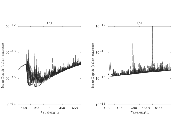
Figure 3: Mass depth ($\rm\Delta M$, total mass above the point of interest) of the line (upper, dashed curve) and continuum (lower, solid curve) formation at monochromatic optical depth $\tau_{\nu}=2/3$ as a function of wavelength in the EUV and far UV.

3 Non-LTE heavy element-rich models with a stratified Fe component

Barstow &  Hubeny (1998) have already reported on the effects of helium stratification in heavy element-rich model atmospheres. They utilised the programme $\rm{\sc tlusty}\>$ (Hubeny 1988; Hubeny &  Lanz 1992, 1995; Lanz et al. 1996) including modifications to allow the abundance of any element at any depth point within an atmosphere to be a completely free parameter. However, to generate a physically realistic model it would be necessary to carry out diffusion calculations for every element. In the case of helium, this is comparatively straightforward. As pointed out by Vennes et al. (1988), the radiation pressure on helium is insufficient to counteract the downward force of gravity to a degree yielding a photospheric helium abundance large enough to explain the observed EUV/soft X-ray flux deficiency, due to the comparatively small number of lines in the EUV waveband. Hence, Vennes et al. (1988) proposed a model where the the relative abundance of He is determined by the equilibrium between ordinary diffusion and gravitational settling and depends on effective temperature, surface gravity and the mass of the overlying H layer. Barstow &  Hubeny (1998) adopted the approach of Vennes et al. (1988) to calculate the depth dependent abundance profile of He for their stratified models and this is also the case in the models used in this work.

For heavier elements, the number of lines found in the EUV is much greater than for helium and radiative forces become important. In these circumstances, simple diffusive equilibrium is no longer an adequate treatment of the relative abundances of the elements. Detailed models dealing with the effects of radiative levitation have been constructed by several workers. Most recently, Chayer, Fontaine &  Wesmael (1995a) and Chayer et al. (1994) have carried out calculations that include all the heavy elements so far found in the atmosphere of G191$-$B2B. Unfortunately, for our purposes, the range of mass depth considered by them, running from $\rm\Delta M/M\approx 10^{-4}$ upto $\approx 10^{-15}$, correponds to a region of the envelope below that of the line/continuum formation depths in the $\rm{\sc tlusty}\>$ models. We note that Chayer et al. (1994) consider the fractional mass depth $\rm\Delta M/M$, whereas we deal with the total mass $\rm\Delta M$, independent of the mass of the star. However, it is a simple matter to convert our scale to theirs by dividing $\rm\Delta M$ by the known mass of G191$-$B2B ($\approx 0.5M_{\odot}$, Marsh et al. 1997a). Hence, with line/continuum formation depths above $\rm\Delta M\approx 3\times 10^{-16}-1\times 10^{-15}$ (corresponding to $\rm\Delta M/M\approx 6\times 10^{-16}-2\times 10^{-15}$), there is little information in the Chayer et al. (1994, 1995a) work that could be usefully incorporated into the $\rm{\sc tlusty}\>$ models.

Since, we have no a priori information on the possible depth dependent abundance of Fe, either from observation or a detailed physical model, we have taken two somewhat arbitrary approaches in an attempt to produce one or more atmosphere models that can match the complete EUVE spectrum of G191$-$B2B. First, we looked at a series of simple ‘slab’ models, where we divide the atmosphere into two or three discrete regions and fix the Fe abundance at a constant value within these depth ranges but allow it to vary from region to region. As starting points we used the nominal Fe abundances determined from the best fit models to the short wavelength and medium wavelength EUVE spectra and placed the slab divisions near the continuum formation depth. We consider models with two and three layers, but it is important to note that the resulting discontinuities are unphysical and that this choice is only a rough attempt to mimic the true depth dependence of the Fe abundance that might be expected from diffusion equilibrium. Table 2 lists the details of the slab models, giving Fe abundances and depth ranges, the quoted depth representing the lower limit of the given abundance for each layer. We note that the abundances of all other elements were constant, as specified in Barstow &  Hubeny (1998; C/H$=2.0\times 10^{-6}$, N/H$=1.6\times 10^{-7}$, O/H$=9.6\times 10^{-7}$, Si/H$=3.0\times 10^{-7}$, Ni/H$=1.0\times 10^{-6}$).

Table 2: Fe abundances and depth structure of slab models computed using $\rm{\sc tlusty}\>$. Depths are in units of $M_{\odot}$.

Model index	Depth top zone	Fe/H	Depth (optional) mid zone	Fe/H	Depth deep zone	Fe/H
fe1	$6.2\times 10^{-16}$	$2\times 10^{-5}$	$1.1\times 10^{-15}$	$1\times 10^{-5}$	$8.3\times 10^{-13}$	$4\times 10^{-6}$
fe2	$6.2\times 10^{-16}$	$2\times 10^{-5}$			$8.3\times 10^{-13}$	$1\times 10^{-6}$
fe3	$6.2\times 10^{-16}$	$3\times 10^{-6}$			$8.3\times 10^{-13}$	$2\times 10^{-5}$
fe4	$6.2\times 10^{-16}$	$3\times 10^{-6}$			$8.3\times 10^{-13}$	$4\times 10^{-5}$
fe5	$6.2\times 10^{-16}$	$1\times 10^{-6}$			$8.3\times 10^{-13}$	$2\times 10^{-5}$
fe6	$6.2\times 10^{-16}$	$1\times 10^{-6}$			$8.3\times 10^{-13}$	$4\times 10^{-5}$
fe9	$6.2\times 10^{-16}$	$5\times 10^{-7}$			$8.3\times 10^{-13}$	$6\times 10^{-5}$
fe10	$6.2\times 10^{-16}$	$1\times 10^{-7}$			$8.3\times 10^{-13}$	$4\times 10^{-5}$
fe11	$6.2\times 10^{-16}$	$1\times 10^{-7}$			$8.3\times 10^{-13}$	$1\times 10^{-4}$
fe12	$4.6\times 10^{-16}$	$1\times 10^{-7}$	$1.4\times 10^{-15}$	$3\times 10^{-6}$	$8.3\times 10^{-13}$	$6\times 10^{-5}$
fe13	$4.6\times 10^{-16}$	$1\times 10^{-7}$	$1.1\times 10^{-15}$	$3\times 10^{-6}$	$8.3\times 10^{-13}$	$6\times 10^{-5}$
fe14	$4.6\times 10^{-16}$	$1\times 10^{-7}$	$8.5\times 10^{-16}$	$3\times 10^{-6}$	$8.3\times 10^{-13}$	$6\times 10^{-5}$
Diffusion/levitation	$M_{H}$	log $\rm g_{rad}$	Reservoir Fe/H
fe7	$10^{-14}$	7.4	$2\times 10^{-4}$
fe8	$10^{-15}$	7.45	$2\times 10^{-4}$

A second approach to modelling the Fe abundance was to modify the diffusion calculation for gravitational settling of helium to deal with Fe (see Vennes et al. 1988; Barstow &  Hubeny 1998). This is straightforward, since the atomic mass and effective charge are free parameters in the calulation and can be adjusted. However, in dealing with helium, it is realistic to assume that there is an infinite reservoir overlaid by a thin H shell, a useful boundary condition. As Fe is not a product of nuclear burning in a white dwarf of normal mass, such as G191$-$B2B, it can only exist as a trace element and the Fe reservoir cannot be specified in the same way. In this case it is necessary to assume that there is some limiting Fe abundance in the deeper layers of the atmosphere. Irrespective of any assumptions about this limiting abundance, what is clear from a range of test diffusion calulations for Fe is that the rate of change of the abundance profile is very steep. That is, for a sensible abundance of Fe at the continuum formation depth, the outer layers are completely depleted of Fe while the Fe abundance in the deeper regions is so high that the emergent EUV flux is negligible. This is not too suprising, as the atomic mass of Fe is fourteen times that of He, and highlights the already well documented fact that radiative levitation effects are necessary to explain the presence of photospheric Fe.

We have not developed a complete radiative levitation calculation for this work but the possible effects can be examined, to first order, by applying a reverse acceleration term in the diffusive equilibrium calculation. Examination of radiative acceleration predictions for Fe (see figure 12 of Chayer et al. 1995a) shows that the value of $\rm g_{rad}$ reaches a plateau-like maximum near the stellar surface. Consequently, we can adopt a constant value for the radiative acceleration term in our calculations. It is important to stress that our choice of log $\rm g_{rad}$ and the reservoir Fe abundance are entirely empirical, based on achieving Fe abundances that approximately correspond to those included in the slab models and which also match the range observed in the homogeneous analysis of section 3 (see table 2).

4 Stratified analysis of the EUV spectrum of G191$-$B2B

In principle, a detailed study of any individual star requires a grid of models to be calculated spanning the possible range of values of all parameters. In practice, this is not feasible for a star like G191$-$B2B because of the number of free parameters that must be considered. A heavy element-rich atmospheric model is specified by $T_{eff}\>$ and log g, plus the abundance of each element included in addition to hydrogen - seven in the models used here. For G191$-$B2B and similar stars, determination of the values of all the parameters is a multi-stage process. Temperature and gravity are estimated from the Balmer lines while abundances can be determined from an analysis of the far UV absorption line strengths. Abundance determinations are typically iterative, with initial estimates made using a first guess at the composition refined by recalculation of a fully converged model. We now know that, to achieve a completely consistent interpretation of the data, it is also necessary to redetermine $T_{eff}\>$ and log g in the light of the measured heavy element abundances (Barstow et al. 1998).

Most analyses performed have made the reasonable simplifying assumption that the stellar envelopes are homogeneous. Once it is necessary to consider depth dependent abundances, the number of possible variables increases dramatically, since it is then necessary to specify the element abundances at each depth point. Since, the models constructed for this work have 70 depth points, this could mean that it is necessary to deal with $\approx 70$ times the number of variables handled in the homogeneous work unless the problem is restricted in some sensible way. The dominant opacity source in the EUV is Fe, therefore, we have chosen to confine the analysis to the study of Fe stratification and assume that all other heavy elements are homogeneously mixed, with the exception of helium which is also stratified as described above and by Barstow &  Hubeny (1998).

Even dealing with a single element it is necessary to define the abundance at 70 depth points and the problem can be reduced further by dividing the atmosphere into a smaller number of discrete regions or slabs or trying to specify a smooth abundance profile with a smaller number of diffusion/levitation parameters, as described in section 3 above. Even so, there is no single variable that can be adjusted to yield the desired result in terms of matching both short and longer wavelength EUVE spectra at the same time. However, from the discussion of the short wavelength problem (section 2), it is at least possible to express the goal as one of steepening the short wavelength region of the spectrum below $\approx 200$Å compared to the longward flux level.

Taking as a starting point the Fe abundances determined from separate fits to short and long wavelength EUV spectra, the model grid listed in table 2 has been constructed in an incremental way, in response to the results of a fit to an earlier model. In each new model, only one or two small changes were made from the previous example, devised to bring the predicted spectrum into closer agreement with that observed (but not always successfully). We consider the results of all these analyses together in table 3, together with the best-fit homogeneous model, for reference. The probability that the best fit model (fe6) is a significant improvement on each of the other models is calculated and listed in table 3. In each case, the entire useful EUV spectrum of G191$-$B2B from 120Å to 600Å was considered. The interstellar column densities were allowed to vary completely freely while H layer mass (for H and He stratification), $T_{eff}\>$ and log g were fixed at their nominal values of $M_{H}=1.2\times 10^{-13}$, 54000K and 7.5 respectively.

Table 3: Best fit values of the interstellar columns and the value of $\chi^{2}_{red}$ (with 584 degrees of freedom)for the grid of models with stratified Fe abundances. The final column gives the probability that model fe6 is a better match to the data than the other model, determined using the F-test. Figures in brackets ($\chi^{2}_{red}$ and F test probability) are the results of fitting the models to two of the strongest FeV lines (1373 and 1376Å) in the IUE spectrum.

Model index	$\rm{H\,{\sc i}}\>$ ($\times 10^{18}$$\rm cm^{-2}\>$)	$\rm{He\,{\sc i}}\>$ ($\times 10^{17}$$\rm cm^{-2}\>$)	$\rm{He\,{\sc ii}}\>$ ($\times 10^{17}$$\rm cm^{-2}\>$)	$\chi^{2}_{red}$	F test probability (% )
Homogeneous	2.15	2.18	1.18	21.0	$>99.99$
fe1	2.02	1.76	7.78	28.2	$>99.99$
fe2	2.09	1.84	5.20	45.4	$>99.99$
fe3	1.96	1.76	4.92	15.8 (1.62)	89.5 (95)
fe4	2.09	2.06	2.21	14.3 (1.75)	31.5 (97)
fe5	1.92	1.67	5.52	17.0 (1.02)	98.6 (42)
fe6	2.05	2.00	2.57	13.8 (1.00)	– (38)
fe9	2.08	2.11	1.22	15.7 (0.89)	87.6 (10)
fe10	2.06	2.11	1.51	15.6 (0.85)	84.8 (–)
fe11	2.14	2.30	0.00	20.3	$>99.99$
fe12	1.73	1.39	16.2	34.0	$>99.99$
fe13	1.76	1.44	7.86	23.8	$>99.99$
fe14	1.87	1.65	4.46	17.0 (1.32)	98.7 (82)
fe7	1.53	1.16	15.1	28.3	$>99.99$
fe8	2.40	2.76	0.00	69.8	$>99.99$

Most of the stratified models offer a significant improvement over that homogeneous model which gives the best match to the EUV spectrum of G191$-$B2B. However, some are rather more successful than others. We examined two different types of slab model, first where the upper layers of the photosphere have the greater Fe abundance and second with this situation reversed. Model fe1, which falls into the former category gives a worse agreement overall, in comparison with the homogeneous case (figure 4). The predicted MW flux clearly falls below the observed level while there is an opposite discrepancy in the SW range. Those slab models where the deeper Fe abundance is greater than that in the outer layers give the best agreement in most cases. The very best of these, model fe6, is a good match to the observed spectrum throughout the complete EUV range (figure 5). Any residual differences are of similar magnitude to those obtained with the homogeneous models when those deal with the more restricted wavelength range above $\approx 180$Å. Neither of the two models which have Fe abundance profiles determined from the balance of radiative levitation and gravitational settling are in good agreement with the observations. For example, the better of these, fe7, requires a very high $\rm{He\,{\sc ii}}\>$ column density to force agreement with the short wavelength flux level. This leaves an unacceptably high flux decrement at and below the 228Å $\rm{He\,{\sc ii}}\>$ Lyman series limit (figure 6).

Figure 4: Comparison of the complete EUVE count spectrum of G191$-$B2B with stratified model fe1 and best-fit interstellar parameters ($\rm{H\,{\sc i}}\>$$=2.02\times 10^{18}$, $\rm{He\,{\sc i}}\>$$=1.76\times 10^{17}$, $\rm{He\,{\sc ii}}\>$$=7.78\times 10^{17}$, $M_{H}=1.3\times 10^{-13}M_{\odot}$, log g$=7.5$, $T_{eff}\>$$=54000$K).

Figure 5: Comparison of the complete EUVE count spectrum of G191$-$B2B with model fe6 that gives the optimum match to the entire wavelength range ($\rm{H\,{\sc i}}\>$$=2.05\times 10^{18}$, $\rm{He\,{\sc i}}\>$$=2.00\times 10^{17}$, $\rm{He\,{\sc ii}}\>$$=2.57\times 10^{17}$, $M_{H}=1.3\times 10^{-13}M_{\odot}$, log g$=7.5$, $T_{eff}\>$$=54000$K).

Figure 6: Comparison of the complete EUVE count spectrum of G191$-$B2B with model fe7 ($\rm{H\,{\sc i}}\>$$=1.53\times 10^{18}$, $\rm{He\,{\sc i}}\>$$=1.16\times 10^{17}$, $\rm{He\,{\sc ii}}\>$$=15.1\times 10^{17}$, $M_{H}=1.3\times 10^{-13}M_{\odot}$, log g$=7.5$, $T_{eff}\>$$=54000$K).

Thus far, the analysis has only addressed the level of agreement between model predictions and observations in the EUV spectral range. However, as the Fe abundances are adjusted at different depths to force agreement with the EUV observations, it is important to consider the effect this has on the predicted Fe line strengths in the far UV. At this point, we can discard those stratified models which do not work and limit the analysis to the selected few that do. Using the F-test, we define this group by assessing which model fits have values of $\chi^{2}_{red}$ which indicate that the probability the fit is significantly worse than the best model (fe6) lies below 99%  (see table 3). The models included are fe3, fe4, fe5, fe6, fe9, fe10 and fe14. Figure 7 shows the a region of the IUE NEWSIPS coadded spectrum of G191$-$B2B spanning the range $\approx 1370$ to 1380Å and including several of the strongest FeV lines. Also shown, in decreasing order of predicted line strength are synthetic spectra computed for models fe4, fe3, fe6, fe9 and fe14. Models fe4 and fe3 are a very good match, with the fe6 and fe9 FeV line strengths being slightly weaker than observed. To assess quantitatively the level of agreement, we have carried out a further analysis, fitting the models predictions to the two strongest FeV lines seen in figure 7 (at 1373.8 and 1376.5Å). The resulting values of $\chi^{2}_{red}$ are listed (in brackets) in table 3, showing that all models are in good agreement with the data and that none can be excluded on the basis of the F test. While model fe6 is the best in the EUV range, fe10, which is not significantly different gives the best match to the far-UV FeV lines.

Figure 7: Coadded IUE echelle spectrum of G191$-$B2B (histogram) spanning the range $\approx 1370$ to 1380Å. Synthetic spectra calculated for models fe4, fe3, fe6, fe9 and fe14 (listed in order of decreasing line strength) are shown for comparison.

5 Discussion

We have been able to provide the first consistent explanation of the complete spectral flux distribution of the hot DA white dwarf G191$-$B2B, including the short wavelength EUV region ($<190$Å) which has previously been problematic, using a grid of atmosphere models with a depth dependent abundance of Fe. Potentially, this is an important breakthrough in our understanding of this and related DAs with significant photospheric heavy element abundances. However, the choice of model structures is somewhat arbitrary, even artificial, in the absence of any a priori physical constraints that we might apply. Hence, it is necessary to re-examine the justification for this approach, question its physical reality and assess the uniqueness of the models before consideration of the possible implications of the results.

In comparison with the homogeneous atmosphere models used in the earlier studies of G191$-$B2B (see figure 1), the stratified models described here seek to suppress the level of the short wavelength ($<190$Å) flux compared to the longer wavelengths, also steepening the spectral slope towards short wavelengths in this region. A number of the models tried were successful, but there may be other mechanisms that might yield a similar effect. Probably the most important question concerns the atomic data included in the models. It is well-known that there are large uncertainties in the continuum and line opacities of the Fe group elements. As the dominant EUV opacity source, the Fe data will be the most critical. However, there are two arguments againts this possibility. First, it seems unreasonable to suppose that any errors should be concentrated in a particular wavelength range. Second, where the greatest uncertainties lie, below $\approx 160$Å, there are very few Fe lines (or of any other species). This might suggest that, in fact, there should be less problem in the short wavelength region. However, we cannot ignore this potential problem completely. Bautista (1996) and Bautista and Pradhan (1997) have computed photoionization cross-section and oscillator strengths for FeIV and FeV, expanding the Opacity Project database by and appreciable number of new transitions. Their calculations take account of transitions between states lying below the first ionization threshold and states lying above. As Bautista and Pradhan note, these transitions can make an important contribution to the total photoabsorption, even though they do not appear as resonances in the photoionisation cross-sections. An alternative explanation for the short wavelength flux decrement is that extra EUV opacity may be present in the form of species, different elements or ionization stages, that have not been taken into account in the models. Again, this seems unlikely, as the few detected elements that we have not included (S and P) are only present in traces too small to have any noticeable effet in the EUV (Vennes et al. 1996). Any elements not yet detected will have still lower abundances.

The choice of stratified models is really determined by the level of complexity that can be accomodated in the modelling process and by the availability of information to determine the abundance depth profile of a given element. The two layer slab models calculated, therefore, represent the simplest possible development of the idea of a depth dependent abundance. Extending this to deal with three layers (models fe1, fe12, fe13, fe14) is a modest increase in complexity, adding two further unknowns (position of the lower layer boundary and the layer abundance) to the three required for two layers. In this work, the additional, narrow layer (2-4 depth points) is used to make a smoother transition between the two main slabs. Generation of a smooth abundance profile is also a result of the diffusion/levitation calculations included in models fe7 and fe8.

It is rather striking that it is the simplest two region slab models that give the best agreement with the data. Of the three layer models, only fe14, where the intermediate layer is reduced to one depth point is in reasonable agreement and the diffusion/levitation models are the worst as a group. One conclusion we could draw from this is that the transition region for the change in Fe abundance is indeed narrow. In addition, the evidence seems to indicate that the Fe abundance is greatest in the deeper layers of the atmosphere but with the abundance in the outer regions being finite and the contrast between the two values being limited to a factor $\approx 50$. For example, the best fit fe6 model (to the EUV data) has a layer abundance ratio of 40, and predicts far UV Fe line strengths that are consistent with the observed spectrum. In comparison, the fe14 model (layer abundance ratio 60), which also gives a good match in the EUV, yields far UV Fe line strengths that are much weaker than observed. This also indicates that the abundance of Fe in the outer layer cannot be less than $\approx 5\times 10^{-7}$.

It is interesting to note that models fe9 and fe10, which are not significantly worse than the best model (fe6), have a lower $\rm{He\,{\sc ii}}\>$ column than any of the other successful models. The resulting He ionization fractions, 37%  and 42%  respectively, are much closer to the 27%  mean value typical of the local ISM (Barstow et al. 1997), compared with either the homogeneous analysis of Lanz et al. (1996; $\approx 80$% ), the stratified H/He work of Barstow &  Hubeny (1998; $\approx 50$%) or the good models considered here (52%  for fe6). On the basis of achieving the lowest He ionization fraction we might favour model fe9 over the others.

However, we must be cautious in taking any of these results too literally, since there are an enormous number of possible, more complex, abundance profiles that we have not yet tested and which might give an equally good or better result. Furthermore, we have only examined the stratification of Fe. There is no reason to assume that this is the only element that might be stratified. Indeed, there is good evidence to show that nitrogen is stratified in the slightly cooler, less heavy element-rich, DA white dwarf REJ1032+532 (Holberg et al. in preparation).

Ideally, we should investigate all these possibilities with new calculations but there is a major problem in producing the large number of models needed. We must seek ways of confining the problem. It may be possible to provide some constraints by measuring abundances using lines that are formed at different depths within the envelope. However, this approach will be particularly sensitive to any uncertainties in the oscillator strengths. Furthermore, as any effects are likely to be quite subtle and the range of uncertainty in determining abundances from far UV line strengths is typically a factor 2, it will be necessary to obtain data of considerably higher signal-to-noise than that currently available. Even then, as examination of the EUV and far UV line formation depths shows (figure 3), it will only be possible to investigate a narrow region of the photosphere, occupying 1 dex in mass depth. Interestingly, there is much more contrast in line formation depth within the EUV and between the EUV and far UV than in the far UV range alone.

If we accept at face value the evidence this work presents, that the Fe in G191$-$B2B is stratified in two main layers with abundances of $\approx 4\times 10^{-5}$ (lower layer) and $\approx 1\times 10^{-6}$ (upper layer), it is interesting to explore the possible implications. A relative depletion of Fe in the outer layers of the envelope may be an indication of ongoing mass-loss in the star. The effects of mass-loss in white dwarf atmospheres has hardly been examined, although there is evidence for this occuring in the hot DO white dwarf REJ0503$-$289 (Barstow &  Sion, 1994). A preliminary study of this problem by Chayer et al. (1993) shows that the outer layers of the envelope will become depleted over time. However, the mass loss rate used in the calculation ($10^{-16}M_{\odot}$/yr) was sufficient to eliminate the reservoir of the heavy elements completely within a few thousand years. On this basis, to see any heavy elements at all, the mass loss rate in G191$-$B2B must be considerably lower. There is clearly a need for new radiative levitation calculations coupled with mass-loss to evaluate this problem properly.

6 Conclusion

We have demonstrated that the complete spectrum of G191$-$B2B can be explained by a model atmosphere where Fe is stratified, with increasing abundance at greater depth. The abundance profile appears to be sharply stepped and may explain the difficulties in matching observed photospheric abundances, usually obtained by analyses utilising homogeneous model atmospheres, to the detailed radiative levitation predictions. Particularly as the latter are only strictly valid for regions deeper than where the EUV/far UV lines and continua are formed. Chayer et al. (1993) show that the outer layers of the envelope will become depleted over time if a weak wind is present. Hence, if found to be the only explanation of the observed spectrum, the relative depletion of Fe in the outer layers of the atmosphere could be the first evidence for radiatively driven mass loss in the star.

In addition, the work presented here may contribute to the resolution of the issue of the possible presence of $\rm{He\,{\sc ii}}\>$ along the line of sight to the star, discussed by Lanz et al. (1996) and Barstow &  Hubeny (1998), and its likely location, in the photosphere or ISM. We find that two of our best stratified models yield an $\rm{He\,{\sc ii}}\>$ column density and He ionization fraction closer to the local ISM values than results obtained in the earlier studies. However, this particular problem will only be completely solved when a much higher resolution spectrum is obtained, capable of separating $\rm{He\,{\sc ii}}\>$ lines from those of heavier elements. We anticipate that the J-PEX spectrometer will provide such data in early 1999 (Bannister et al. 1999). Through its ability to study individual lines, this instrument may also be able to deliver new information on the stratification of Fe and other elements.

References

- [19] Bannister N.P., Cruddace, R.G., Kowalski, M., Fritz, G., Barstow M.A., Fraser G.W., Barbee, T., Lapington J.S., Tandy J., 1999, in the proceedings of the 11th European Workshop on White Dwarfs, ed. J-E. Solheim, ASP Conference Series, in press
- [19] Barstow M.A. et al., 1993, MNRAS, 264, 16
- [19] Barstow M.A., Dobbie, P.D., Holberg J.B., Hubeny I., Lanz T., 1997a, MNRAS, 286, 58
- [19] Barstow M.A., Holberg J.B., Hubeny I., Lanz T., 1997b, in White Dwarfs, eds. J. Isern, M. Hernanz and E. Garcia-Berro, Kluwer, in press
- [19] Barstow M.A., Holberg J.B., Koester D., 1995, MNRAS, 274, L31
- [19] Barstow M.A., Hubeny I., 1998, MNRAS, 299, 379
- [19] Barstow M.A., Hubeny I., Holberg J.B., 1998, MNRAS, in press
- [19] Barstow M.A., Hubeny I., Lanz T., Holberg J.B., Sion E.M., 1996, in Astrophysics in the Extreme Ultraviolet, eds. S. Bowyer and R.F. Malina, Kluwer, 203
- [19] Barstow M.A. Sion E.M., 1994, MNRAS, 271, L52
- [19] Bautista M.A., 1996, A& ASS, 199, 105
- [19] Bautista M.A., Pradhan A.K., 1997, A& ASS, 126, 365
- [19] Bruhweiler F.C., Kondo Y. 1981, ApJ, 248, L123
- [19] Bruhweiler F.C., Kondo Y. 1983, ApJ, 269, 657
- [19] Chayer P., LeBlanc F., Fontaine G., Wesemael F., Michaud G., Vennes S., 1994, ApJ, 436, L161
- [19] Chayer P., Fontaine G., Wesemael F., 1995a, ApJS, 99, 189
- [19] Chayer P., Pelletier C., Fontaine G., Wesemael F., 1993, in ‘White Dwarfs: Advances in Observation and Theory’, ed M.A. Barstow, Kluwer, Dordrecht, 261.
- [19] Chayer P., Vennes S., Dupuis J., Pradhan A.K., 1997, in ‘White Dwarfs’, eds. J. Isern, M. Hernanz and E. Garcia-Berro, Kluwer, Dordrecht, 273
- [19] Chayer P., Vennes S., Pradhan A.K., Thejll P., Beauchamp A., Fontaine G., Wesemael F., 1995b, ApJ, 454, 429
- [19] Cunto W., Mendoza C., Ochsenbein F., Zeippen C.J., 1993, A& A, 275, L5
- [19] Dupuis J., Vennes S., Bowyer S., Pradhan A.K., Thejll P., 1995, ApJ, 455, 574
- [19] Koester D., Wolff B., Jordan S., Dreizler S., 1997, in “Proceedings of the 3rd Conference on Faint Blue Stars”, in press.
- [19] Holberg J.B., Hubeny I., Barstow M.A., Lanz T., Sion E.M., Tweedy R.W., 1994, ApJ, 425, L105
- [19] Hubeny I., 1988, Comp.Phys.Comm., 52, 103
- [19] Hubeny I., Lanz T., 1992, A& A, 262, 501
- [19] Hubeny I., Lanz T., 1995, ApJ, 439, 875
- [19] Kurucz R.L., 1988, in IAU Trans., ed. M. McNally, VolXXB, Kluwer, Dordrecht, 168
- [19] Lanz T., Barstow M.A., Hubeny I., Holberg J.B., 1996, ApJ, 473, 1089
- [19] Marsh, M.C. et al., 1997a, MNRAS, 286, 369
- [19] Marsh, M.C. et al., 1997b, MNRAS, 287, 705
- [19] Press W.H., Teulosky S.A., Vetterling W.T., Flannery B.P., 1992, Numerical Recipes (2nd edition), p687ff, Cambridge
- [19] Rumph T., Bowyer S., Vennes S., 1994, AJ, 107, 2108
- [19] Sion, E.M., Bohlin, R.C., Tweedy, R.W., Vauclair, G.P. 1992, ApJ, 391, L29
- [19] Vennes S., Chayer P., Hurwitz M., Bowyer S., 1996, ApJ, 468, 989
- [19] Vennes S., Chayer P., Thorstensen J.R., Bowyer S., Shipman H.L., 1992, ApJ, 392, L27
- [19] Vennes S., Pelletier C., Fontaine G., Wesmael F., 1988, ApJ, 331, 876
- [19] Wolff B., Koester D., Jordan S., Haas S., 1998, A& A, 329, 1045
- [19]