Nonradial and nonpolytropic astrophysical outflows
IV. Magnetic or thermal collimation of winds into jets?

Abstract

An axisymmetric MHD model is examined analytically to illustrate some key aspects of the physics of hot and magnetized outflows which originate in the near environment of a central gravitating body. By analyzing the asymptotical behaviour of the outflows it is found that they attain a variety of shapes such as conical, paraboloidal or cylindrical. However, non cylindrical asymptotics can be achieved only when the magnetic pinching is negligible and the outflow is overpressured on its symmetry axis. In cylindrical jet-type asymptotics, the outflowing plasma reaches an equilibrium wherein it is confined by magnetic forces or gas pressure gradients, while it is supported by centrifugal forces or gas pressure gradients. In which of the two regimes (with thermal or magnetic confinement) a jet can be found depends on the efficiency of the central magnetic rotator. The radius and terminal speed of the jet are analytically given in terms of the variation across the poloidal streamlines of the total energy. Large radius of the jet and efficient acceleration are best obtained when the external confinement is provided with comparable contributions by magnetic pinching and thermal pressure. In most cases, collimated streamlines undergo oscillations with various wavelengths, as also found by other analytical models. Scenarios for the evolution of outflows into winds and jets in the different confinement regimes are shortly outlined.

Key words MHD – plasmas – solar wind – stars: mass loss – stars: pre-main sequence – ISM: jets and outflows – Galaxies: jets

1 Introduction

Nonuniform plasma outflows seem to be ubiquitous in astrophysics on galactic and extragalactic scales. The closest example is the solar wind itself which shows strong heliolatitudinal velocity gradients as recently observed by Ulysses (Lima & Tsinganos 1996, McComas et al. 1998). Further away collimated outflows are observed in association with several galactic objects, such as young and evolved stars, planetary nebulae, X-ray binaries and collapsed objects (for reviews see Ray 1996, Kafatos 1996, Mirabel & Rodriguez 1996, Brinkmann & Müller 1998, Livio 1998). Finally, on extragalactic scales jets are observed to originate in many Active Galactic Nuclei and Quasars (Biretta 1996, Ferrari et al. 1996).

Yet, despite their abundance the basic questions on the formation, acceleration and propagation of nonuniform winds and jets have not been fully answered. Nevertheless, observations seem to indicate that the basic ingredients for producing astrophysical outflows are some sort of heating to launch thermally the wind at the axis plus a rotating central gravitating object and/or an accretion disk threaded with magnetic fields to accelerate magnetocentrifugally and collimate the outflow.

1.1 Drivers of the collimated plasma outflow

Several mechanisms have been investigated for accelerating and collimating astrophysical outflows in galactic and extragalactic scales. Magnetic rotator forces seem to play a rather dominant and crucial role (Lynden-Bell 1996) but they are probably not the only relevant mechanism.

First, thermally driven models are based on the de Laval nozzle analogy of the solar wind (Parker 1963, Liffman & Siora 1997). This requires the presence of a hot corona around the central body of the YSO or the AGN. X-ray emission detected in several of these objects may imply that thermal effects contribute to the general acceleration mechanism at the base of the flow but they are probably not the only ingredient. Furthermore, if the wind is associated to a very bright object, the flow can be effectively accelerated by the photon flux (radiatively driven winds, Cassinelli 1979). Parallely note also that collimation of bipolar outflows from YSOs and Planetary Nebulae by external thermal pressure gradients have been extensively studied in the frame of the Generalized Wind Blown Bubble scenario (GWBB, Frank 1998). It has demonstrated successfully that magnetic processes may not be the only way to achieve collimated outflows.

Second, magnetic pressure driven models are based on the uncoiling spring analogy and have been examined by Draine (1983), Uchida & Shibata (1985) and Contopoulos (1995). There, it is assumed that a toroidal magnetic field $B_{\phi}$ is created and highly amplified by the winding-up of its field lines by a radially collapsing and non-Keplerian rotating disk. Plasma is then accelerated from the disk in the poloidal direction by the action of the resulting torsional Alfvén waves.

Third, magnetocentrifugally driven outflow models are based on the classical bead on a rotating rigid wire analogy. There, the magnetized cold fluid is flung out (even to relativistic velocities) from the surface of the Keplerian accretion disk, provided that the poloidal field lines are inclined enough with respect to the disk axis (Blandford & Payne 1982, Pelletier & Pudritz 1992, Contopoulos & Lovelace 1994, Cao 1997). This approach is suitable to model winds from accretion disks, but is not valid around the symmetry axis. Moreover it has been pointed out recently (Ogilvie & Livio 1998) that, even if the lines are sufficiently inclined, a potential barrier still exists that can be overcome only by the presence of an extra source of energy (e.g. a hot corona).

In all the above treatments the effects of the combination of gas pressure and magnetic fields in accelerating, collimating and confining jets have not been discussed adequately, despite the fact that the role of the gas pressure has been recognized for a long time, i.e., that jets are not moving in a vacuum (molecular clouds around YSO’s, or host galaxies in AGN) and hence they must have some interaction with the external medium (Ferrari et al. 1996; Frank 1998). This approach may also highlight the transition from fully thermally driven to fully magnetocentrifugally driven collimated winds.

1.2 Radially self-similar models

As with any fully MHD approach and despite of the simplifications of steadiness and axisymmetric geometry, several approximations are still unavoidable in order to obtain exact solutions useful for an understanding of the MHD mechanism for the initial acceleration and final collimation. Thus, one simple analytical way out is the use of self-similarity. This hypothesis allows an analysis in a 2-D geometry of the MHD equations which reduce then to a system of ordinary differential equations. The basis of the self-similarity treatment is the assumption of a scaling law of one of the variables as function of one of the coordinates. The choice of the scaling variable depends on the specific astrophysical problem.

Several models self-similar in the radial direction have been investigated to analyze the structure of winds from accretion disks (Blandford & Payne 1982, Contopoulos & Lovelace 1994, Li et al. 1992, Li 1995, 1996, Ferreira 1997, Ostriker 1997). In these models the driving force and the collimation derive from a combination of the magnetic and centrifugal forces. Moreover, as disc-winds are associated with jets, these studies usually do not consider under which parametric conditions full collimation is obtained. Exceptions are given in Pelletier & Pudritz (1992) and Contopoulos & Lovelace (1994) where the collimation efficiency is linked to a current flowing in agreement with the Heyvaerts & Norman (1989) general analysis. However, the absence of an exact crossing of all the existing critical points in the solutions presented in these papers prevents from considering their conclusions as definitive. Nevertheless, it has been shown that within the frame of self-similar disc-wind assumptions, it is possible to cross all critical points thus getting meaningful solutions (Tsinganos et al. 1996, Vlahakis 1998). Moreover, the role of the inhomogeneity in the pressure distribution has not been taken into account until recently in these models (Ferreira 1997) and a full parametric study of this extra variable is yet to be performed.

1.3 Meridionally self-similar models

In a series of studies, solutions of the MHD equations that are self-similar in the meridional direction have been also analyzed (Tsinganos & Trussoni 1990, 1991, Tsinganos & Sauty 1992a,b, Papers I and II of this series, Trussoni & Tsinganos 1993, Sauty & Tsinganos 1994, Paper III of this series, Trussoni et al. 1997, henceforth TTS97). Such a treatment allows to study the physical properties of the outflow close to its rotational axis. As in this region the contribution to acceleration of the magnetocentrifugal forces is small, the effect of a thermal driving force is essential. This implies also that the structure of the gas pressure in the flow is essential.

Two main classes of such self similar solutions have been investigated depending on whether the components of the pressure gradient along the radial and meridional directions are related or not. In the second case the shape of the streamlines and fieldlines is prescribed ‘a priori’, and the main features of the dynamical variables are self-consistently deduced from the integration. In particular, it has been shown that acceptable solutions for magnetized flows with asymptotic superAlfvénic velocity exist only when rotation is included (Tsinganos & Trussoni 1991, Trussoni & Tsinganos 1993, TTS97). As a consequence of this study it seems that even pressure confined jets from slow magnetic rotators need magnetic fields and rotation.

In the other case, in which the two components of the gas pressure are related, the structure of the streamlines is deduced as a self-consistent solution of the MHD equations. It has been shown (Papers I and II) that hydrodynamical and nonrotating magnetized winds are always radially expanding from the source. On the other hand, rotating magnetized flows with a spherically symmetric structure for the pressure gradient can have final superAlfvénic velocities with either radial or collimated asymptotically streamlines, depending on the values of the parameters (Paper III). This allows to deduce a criterium to select conically expanding winds from cylindrically collimated jets (Sauty et al. 1996).

1.4 Plan of this paper

We extend here the analysis of Paper III to the more general case of solutions for rotating magnetized winds with a nonspherically symmetric gas pressure. In the present paper we concentrate on the asymptotic analysis and its link to the initial boundary conditions: this allows us to derive a general criterion for the collimation of winds into jets. The analysis of the properties of the complete numerical solutions deserves a separate study which is postponed to a following paper.

In Sec. 2 we summarize the properties of the meridional self-similar MHD equations while in Sec. 3 we discuss the energetic structure of the outflow. In particular we show that an energy integral exists that links the asymptotic regime to the boundary conditions at the base, allowing to formulate a general criterion for the collimation of the wind. The different physical conditions for asymptotic confinement (magnetic or thermal) are discussed in detail in Sec. 4, and in Sec. 5 we show that oscillating configurations can be present in cylindrically collimated jets. In Sec. 6 the equilibrium asymptotic properties of non collimated flows are outlined, while in Sec. 7 we summarize the results and shortly discuss the astrophysical implications of our analysis.

2 Meridionally self-similar MHD model

2.1 Steady axisymmetric ideal MHD outflows

The global dynamical properties of cosmic winds and jets are usually analyzed by assuming that they represent outflows of a fully ionized plasma with a bulk speed $\vec{V}$ and carrying a magnetic field $\vec{B}$ in the gravitational field of a central body of mass $\cal M$. The familiar MHD equations are employed for a physical description of these phenomena. In particular, under steady and axisymmetric conditions ($\partial/\partial t=\partial/\partial\varphi=0$), the MHD equations are known to admit certain free integrals, i.e., functions which remain constant on the magnetic surfaces generated by the revolution around the magnetic/flow symmetry axis of the system of a poloidal magnetic line $A(r,\theta)$ = constant (Tsinganos 1982). Specifically, on the surface of such a flux tube $A$ = const., the following physical quantities remain invariant throughout the extent of these surfaces from the base to infinity:

• $\Psi_{A}$(A), the ratio of the magnetic and mass fluxes,

• $L(A)$, the total specific angular momentum carried by the flow and the magnetic field,

• $\Omega(A)$, the corotation frequency or angular velocity of each streamline at the base of the flow.

Furthermore, it is well known that the poloidal ($p$) and azimuthal (toroidal, $\varphi$) components of the magnetic field and the velocity can be expressed in terms of these free integrals and the poloidal Alfvén Mach number, using spherical ($r,\theta,\varphi$) or cylindrical ($\varpi,\varphi,z$) coordinates (for details see Paper III). In particular, the poloidal Alfvén Mach number (or Alfvén number) $M$ is,

$$M^{2}=4\pi\rho{{V^{2}_{p}}\over{B^{2}_{p}}}={{\Psi^{2}_{A}}\over{4\pi\rho}}\,.$$

On the other hand, the two integrals $L(A)$ and $\Omega(A)$ are not independent if the flow is transalfvénic. In such a case, at the cylindrical distance $\varpi_{a}$ of the Alfvén point ($M=1$) from the field/flow axis of a flux tube labeled by $A$ they are related as $\varpi_{a}^{2}(A)=({r_{*}\,{\sin}\theta_{a}})^{2}=L/\Omega$.

2.2 Generalized Bernoulli integral

A fourth constant of the motion expresses the conservation of energy along streamlines. Thus, by projecting the momentum equation along a streamline, taking into account the first law of thermodynamics for energy conservation, we obtain the generalized classical Bernoulli integral (Paper III),

$$E(A)={1\over 2}V_{\rm p}^{2}+{1\over 2}V_{\varphi}^{2}-{{\cal G}{\cal M}\over r}-{\Omega\,\over\Psi_{A}}\varpi B_{\varphi}+h-\Theta_{r_{o}}^{r}(A)\,,$$

where

$$\Theta_{r_{o}}^{r}(A)=\int_{r_{o}}^{r}{q(r^{\prime},A)\over\rho(r^{\prime},A)V_{r}(r^{\prime},A)}{\rm d}r^{\prime}\,,$$

$h$ is the enthalpy of the perfect monoatomic gas ($\Gamma=5/3$), $q$ is the net local volumetric heating/cooling rate, and ${\cal G}$ the gravitational constant. Thus, at a given radial distance $r$ along the streamline labeled by $A$, the conserved energy $E(A)$ represents the sum of the kinetic, gravitational, Poynting and ideal thermal energy flux densities per unit of mass flux density, minus the extra heat received by the flow between the anchored footpoint at a basal radial distance $r_{o}$ and the point $r$ under consideration, $\Theta_{r_{o}}^{r}(A)$.

2.3 Self-similarity: scaling laws for the variables

The model analysed in this paper belongs to the wide class of meridionally self-similar MHD equilibria (see also Trussoni et al. 1996; Tsinganos et al. 1996; TTS97; Vlahakis & Tsinganos 1998, henceforth VT98). In the following we briefly summarize the main steps for the construction of such a model (see Appendix A for more technical details).

For convenience, first of all the variables are normalized to their respective values at the Alfvén surface along the axis of rotation, $r=r_{*}$. In particular, we define the dimensionless radial distance $R=r/r_{*}$ and the Alfvén speed $V^{2}_{*}=B^{2}_{*}/4\pi\rho_{*}$, where $B_{*}$, $V_{*}$ and $\rho_{*}$ are the poloidal magnetic field, poloidal velocity and density along the polar axis at the characteristic radius $r_{*}$. For the magnetic flux function $A$ we define its dimensionless form by

$$\alpha(R,\theta)={A(r,\theta)\over 2r^{2}_{*}B_{*}}\,.$$

Note that along the polar axis $\alpha(R,0)=0$. To obtain the final expressions for the physical variables, we make the following crucial assumptions:

• First, we assume that the Alfvén surface is spherical, $M=M(R)$. Then, according to Eq. (2.1), the density can be expressed as the product of a function of $R$ [i.e. $1/4\pi M^{2}(R)$] and a function of $\alpha$ [i.e. $\Psi_{A}^{2}(\alpha)$]. Furthermore, we Taylor expand the function $\Psi^{2}_{A}(\alpha)$ to the first order in $\alpha$ such that the variation of the density on a spherical surface of given radius $R$ is proportional to the magnetic flux $\alpha$.

• Second, we assume that the magnetic flux function $\alpha$ is expressed as the product of a function of $R$ and a function of $\theta$. Furthermore, for the function of $\theta$ we take a dipolar dependence with the colatitude $\theta$. This immediately implies that the Alfvén cross sectional area $\pi\varpi_{a}^{2}$ of a flux surface is proportional to the corresponding magnetic flux $\alpha$. Also, the ratio $G^{2}=\varpi^{2}/\varpi_{a}^{2}$ of the cross sectional area of the flux tube to the Alfvén cross sectional area of the same flux tube depends solely on the radial distance $R$.

• Third, we assume that the total axial current $I_{z}$ enclosed by a flux tube $\alpha$ = const. is proportional to the corresponding magnetic flux. This assumption fixes the angular momentum integral $L$ (Paper III). Note that at once the integral of the corotation frequency $\Omega$ follows from its relation with $L$ at the Alfvén distance, $L=\Omega\varpi_{a}^{2}$. Note also that the integrals $L$ and $\Omega$ are chosen such that $L\Psi_{A}$ and $L\Omega\Psi_{A}^{2}$ contain only first order $\alpha$-terms, in analogy with the previous assumptions.

• Fourth, we assume that the $\alpha$-dependence of the gas pressure is similar to that of the density distribution. This means that the pressure is ultimately a function of the density along a given magnetic surface, a situation analogous to the often used polytropic assumption. However, this implicit relationship between pressure and density is much more general than the somehow artificial polytropic assumption. Contrary to the polytropic relation, its exact form is not imposed a priori but is determined by the full solution.

Altogether, the four main assumptions of this meridionally self-similar model can be summarized as follows,

$$\rho(R,\alpha)={\rho_{*}\over M^{2}(R)}(1+\delta\alpha)\,,\;\Psi_{A}^{2}=4\pi\rho_{*}(1+\delta\alpha)\,,$$

$$\varpi^{2}(R,\alpha)=r^{2}_{*}G^{2}(R)\alpha\,,\qquad\varpi_{a}^{2}(\alpha)=r^{2}_{*}\alpha\,,$$

$$L\Psi_{A}=\lambda r_{*}B_{*}\alpha\,,\qquad L\Omega\Psi_{A}^{2}=\lambda^{2}B_{*}^{2}\alpha\,,$$

$$P(R,\alpha)={1\over 2}\rho_{*}V^{2}_{*}\Pi(R)(1+\kappa\alpha)\,.$$

The introduced parameters $\delta$, $\kappa$ and $\lambda$ measure the variation with the colatitude of the density, pressure and rotation, respectively. A fourth parameter $\nu$ enters from the momentum equation as the ratio, at the Alfvén distance along the polar axis, of the escape speed to the flow speed there,

$$\nu^{2}={2{\cal G}{\cal M}\over r_{*}V^{2}_{*}}\,.$$

2.4 Magnetic rotator energy

An important physical quantity in magnetized outflows is the so called magnetic rotator energy (Michel 1969, Belcher & McGregor 1976),

$$E_{\rm MR}=\Omega L\,.$$

The basal Poynting energy $E_{{\rm Poynt.},o}$, defined as the ratio of the Poynting flux density $S_{z}$ per unit of mass flux density $\rho V_{z}$, is roughly equal to the magnetic rotator energy $\Omega L$ if at the base the radius of the jet is much smaller than the Alfvén radius ($G_{o}\ll 1)$ and the Alfvén number there is also negligibly small ($M_{o}\ll 1$),

$$E_{{\rm Poynt.},o}={S_{z}\over\rho V_{z}}\Bigl{|}_{o}=\Omega L{1-G_{o}^{2}\over 1-M_{o}^{2}}\approx\Omega L\,.$$

Let $E_{o}$ be the sum of the kinetic, gravitational and thermal energies per unit mass at the base of the outflow. Then the total available energy for the outflow at the base is $E\approx E_{o}+\Omega L$. Accordingly, we have an outflow from a Fast Magnetic Rotator (FMR) when $E_{o}\ll\Omega L$ and an outflow from a Slow Magnetic Rotator (SMR) in the opposite case of $E_{o}\gg\Omega L$.

2.5 Solving the self-similar MHD equations

In order to solve the resulting MHD equations, it is useful to introduce an extra function $F(R)$ (Papers II and III),

$$F(R)=2\left(1-{{\rm d}\,\ln G(R)\over{\rm d}\,\ln R}\right)\,.$$

Evidently, while $G(R)$ defined in Eq. (2.3b) measures the dimensionless cylindrical radius of a flux tube at the distance $R$, $F(R)$ is simply giving the expansion factor of the streamlines. The limiting case $F(R)=0$ corresponds to conical expansion and radial fieldlines, while for $F(R)=2$ we have cylindrical expansion parallel to the axis (collimation). In between these two regimes the flow is paraboloidal.

The above assumptions, Eqs. (2.3), immediately give the components of the velocity and magnetic fields (Eqs. A.3 in Appendix A). On the other hand, the momentum conservation law in combination with the above assumptions gives four ordinary differential equations for the four variables $M^{2}(R)$, $F(R)$, $\Pi(R)$ and $G(R)$ (see Appendix A for details).

The complete solution of these equations, from the base of the outflow to infinity, with the required crossing of all appropriate critical points, is indeed an interesting undertaking and worth of a separate paper. Here instead, we shall concentrate on some novel results obtained solely by solving the equations asymptotically far from the Alfvén surface ($R\gg 1$) and taking into account the boundary conditions on the source.

3 The energy integral and collimation criterion

3.1 The generalized Bernoulli integral

A nonadiabatic flow of a monoatomic gas with ratio of specific heats $\Gamma=5/3$ is always heated at a net volumetric rate $q$

$$q=\rho\vec{V}\cdot\left(\nabla h-{{\nabla P}\over{\rho}}\right)\,,\quad h={\Gamma\over\Gamma-1}{P\over\rho}\,.$$

With expressions (2.3a) and (2.3d) for the gas density and pressure, it follows immediately that this heating can be written as (see Sec. 5 in Paper III for details of the derivation),

$${q(R,\alpha)\over\rho(R,\alpha)V_{r}(R,\alpha)}={V_{*}^{2}\over 2r_{*}}{1+\kappa\,\alpha\over 1+\delta\,\alpha}{\cal Q}(R)\,,$$

where the dimensionless specific heating rate per unit of radial length along a given streamline is,

$${\cal Q}(R)={1\over\Gamma-1}\left[M^{2}{\hbox{d}\Pi\over\hbox{d}R}+\Gamma\Pi{\hbox{d}M^{2}\over\hbox{d}R}\right]\,.$$

Hence, the generalized classical Bernoulli integral (2.2) takes the simpler form

$$E(\alpha)={1\over 2}V_{*}^{2}{{\cal E}+\alpha\Delta{\cal E}\over 1+\delta\alpha}\,,$$

where the two constants ${\cal E}$ and $\Delta{\cal E}$ represent the polar specific energy and the variation across a streamline of the specific energy, respectively (in Paper III ${\cal E}$ was denoted by ${\cal F}_{1}$, $\Delta{\cal E}$ by ${\cal F}_{2}$ and ${\cal Q}$ by ${\cal Q}_{1}$).

It is straightforward to show from Eqs. (2.2), (2.3), (A.3) and (3.1)–(3.2) that ${\cal E}$ and $\Delta{\cal E}$ have the following analytical expressions (Paper III)

$${\cal E}={M^{4}\over G^{4}}-{\nu^{2}\over R}+{\Gamma\over\Gamma-1}\Pi M^{2}-\int_{R_{o}}^{R}{\cal Q}(R)dR\,,$$

$$\Delta{\cal E}={M^{4}\over R^{2}G^{2}}\left[{F^{2}\over 4}-1\right]-{\delta\,\nu^{2}\over R}+{\lambda^{2}\over G^{2}}\left[M^{2}-G^{2}\over 1-M^{2}\right]^{2}$$

$$+2\lambda^{2}\left[1-G^{2}\over 1-M^{2}\right]+\kappa\left[{\Gamma\over\Gamma-1}\Pi M^{2}-\int_{R_{o}}^{R}{\cal Q}(R)dR\right]\,.$$

It is worth to digress for a moment and try to get some insight into the physical meaning of these two conserved components of the specific energy, ${\cal E}$ and $\Delta{\cal E}$.

3.1.1 Polar specific energy

In the first expression, Eq. (3.3a), the polar energy flux $\cal E$ is composed of four terms which are successively the poloidal (i.e. radial here) kinetic and gravitational energies, the enthalpy and the heating along the polar axis.

The polar specific energy ${\cal E}$ can be evaluated at both the base of the wind $R_{o}$ and far from it as $R\longrightarrow\infty$,

$${\cal E}=-{\nu^{2}\over R_{o}}+{\Gamma\over\Gamma-1}\Pi_{o}M_{o}^{2}\,$$

$$={M_{\infty}^{4}\over G_{\infty}^{4}}+{\Gamma\over\Gamma-1}\Pi_{\infty}M_{\infty}^{2}-\int_{R_{o}}^{\infty}{\cal Q}(R)dR\,.$$

At the base, wherein the kinetic energy of the outflow is negligible, Eq. (3.4a) shows that the polar energy has basically two terms: the gravitational energy and the initial input of thermal energy in the form of enthalpy. On the other hand, at infinity, Eq. (3.4b), the conserved polar specific energy is composed of the final kinetic energy along the polar axis and the terminal enthalpy minus the additional extra heating which the flow has received during its propagation from $R_{o}$ to infinity.

Note that if the wind is cylindrically collimated, $M_{\infty}$, $G_{\infty}$ and $\Pi_{\infty}$ have finite values. In all other cases, $M_{\infty}$ and $G_{\infty}$ may be unbounded, although their ratio, which is the polar speed in units of the Alfvén speed, should remain finite,

$${M_{\infty}^{2}\over G_{\infty}^{2}}={V_{\infty}\over V_{*}}\,.$$

Moreover the terminal pressure $\Pi_{\infty}$ vanishes unless the integral of the heating diverges, a rather unphysical situation corresponding to an infinite input of heat.

The conservation of the polar energy simply expresses the fact that the flow along the polar axis is thermally driven. Furthermore, from Eqs. (3.4a,b) it becomes evident how the conversion of the heat content of the plasma into kinetic and gravitational energy maintains the outflow,

$${\Gamma\over\Gamma-1}(\Pi_{o}M_{o}^{2}-\Pi_{\infty}M_{\infty}^{2})+\int_{R_{o}}^{\infty}{\cal Q}(R)dR$$

$$={\nu^{2}\over R_{o}}+{M_{\infty}^{4}\over G_{\infty}^{4}}\,.$$

In other words, the decrease of the enthalpy at infinity together with the external heat input integrated along the polar streamline, on one hand lifts the gas out of the gravitational potential well and on the other, gives to it a finite terminal speed. Of course, this is nothing more than the classical picture of the Parker thermally driven wind.

3.1.2 Variation of the specific energy across streamlines

The second conserved component $\Delta{\cal E}$ of the specific energy gives the excess or deficit of the volumetric total energy $E$ at a nonpolar streamline as compared to the corresponding energy at the polar axis and the same spherical distance, normalized to the volumetric energy of the magnetic rotator. Thus, $\Delta{\cal E}$ has five contributions which correspond to the five different terms appearing successively in the RHS of Eq. (3.3b). Each one represents the variation – in units of the volumetric energy of the magnetic rotator – between any streamline and the polar axis of (i) the poloidal kinetic energy, (ii) the volumetric gravitational energy, (iii) the azimuthal kinetic energy (which is zero along the polar axis), (iv) the Poynting flux (which is also zero along the polar axis) and (v) the thermal content (enthalpy plus heating; see Appendix B for details).

In a more compact way we may write $\Delta{\cal E}$ as follows,

$${\Delta{\cal E}\over 2\lambda^{2}}={\rho(R,\alpha)E(\alpha)-\rho(R,{\rm{pole}})E({\rm{pole}})\over\rho(R,\alpha)L(\alpha)\Omega(\alpha)}\,.$$

Evidently, ${\Delta{\cal E}/2\lambda^{2}}$ represents the variation across the flow of the total volumetric energy in units of the volumetric energy of the magnetic rotator. Therefore, the sign of $\Delta{\cal E}$ determines whether there is a deficit of energy per unit volume (and not per unit mass) along the polar streamline as compared to the other streamlines (case $\Delta{\cal E}>0$) or an excess of energy in the polar streamline as compared to the other nonpolar streamlines (case $\Delta{\cal E}<0$).

Furthermore, $\Delta{\cal E}/2\lambda^{2}$ can be expressed (see Appendix B for more comments) in terms of the conditions at the source boundary $R_{o}$ where the cylindrical radius is $\varpi_{o}(\alpha)$, the escape speed $V_{esc,o}$, the polar density $\rho_{o}({\rm{pole}})$ and the density at any other streamline $\rho_{o}(\alpha)$:

$${\Delta{\cal E}\over 2\lambda^{2}}={\Delta\left[\rho_{o}(E_{{\rm Poynt.},o}+E_{{\rm R},o}+h_{o}+E_{\rm G,o})\right]\over\Delta(\rho E_{\rm{MR}})_{o}}\,,$$

where $\Delta(\rho E_{\rm{MR}})_{o}$ is the variation of the energy of the magnetic rotator, $\Delta(\rho E_{\rm Poynt.})_{o}$ is the variation of the Poynting energy, $\Delta(\rho E_{\rm R})_{o}$ is the variation of the rotational energy at the base, $\Delta(\rho E_{\rm G})_{o}$ is the variation of the volumetric gravitational energy at the base and $\Delta(\rho h)_{o}$ is the variation of the volumetric thermal flux at the base, respectively,

$$\Delta(\rho E_{\rm{Poynt}})_{o}=\rho_{o}(\alpha)E_{{\rm Poynt},o}(\alpha)=\rho_{o}(\alpha)(\Omega L-\Omega^{2}\varpi_{o}^{2})\,,$$

$$\Delta(\rho E_{\rm R})_{o}=\rho_{o}(\alpha)E_{{\rm R},o}(\alpha)=\rho_{o}(\alpha){V_{\varphi,o}^{2}\over 2}=\rho_{o}(\alpha){\varpi_{o}^{2}\Omega^{2}\over 2}\,,$$

$$\Delta(\rho E_{\rm G})_{o}=-{{\cal G}{\cal M}\over r_{o}}\left[\rho_{o}(\alpha)-\rho_{o}({\rm{pole}})\right]\,,$$

$$\Delta(\rho h)_{o}={\Gamma\over\Gamma-1}[P_{o}(\alpha)-P_{o}({\rm{pole}})]\,,$$

$$\Delta(\rho E_{\rm MR})_{o}=\rho_{o}(\alpha)E_{\rm MR}(\alpha)=\rho_{o}(\alpha)L(\alpha)\Omega(\alpha)\,.$$

In this notation, $\Delta$ always denotes a variation across the fieldlines at a given radial distance $R$, i.e. $\Delta y=y(R,\alpha)-y(R,{\rm pole})$ for every function $y(R,\alpha)$.

In Eq. (3.7a) note that (see also Eqs. 2.5)

$$E_{{\rm Poynt.},o}+E_{{\rm R},o}=E_{\rm{MR}}-E_{{\rm R},o}>0\,.$$

The Poynting flux plus the rotational energy is simply the energy of the magnetic rotator minus the rotational energy. This last form is the one used in Paper III. In other words, and even in the slow magnetic rotator limit, the rotational energy never exceeds the energy of the magnetic rotator.

3.2 Energetic definition of Efficient/Inefficient Magnetic Rotators

At this point we inevitably note that ${\cal E}$ and $\Delta{\cal E}$ are two inconvenient constants because their absolute values depend on the integration of the total heating supply and so they can be evaluated only after the problem has been solved and the required heating can be calculated. However these two constants are related to each other. In fact, the last two terms in the expression of $\Delta{\cal E}$ in Eq. (3.3b), which correspond to the transverse variations of enthalpy and heating, are identical to the last two terms of ${\cal E}$ within a factor of $\kappa$. Evidently, this is due to the assumptions on the pressure and density distribution, Eqs. (2.3a,d). These initial assumptions imply the existence of an implicit relationship between the latitudinally normalized pressure and density,

$${P(R,\alpha)\over P(R,0)}=1+{\kappa\over\delta}\left[{\rho(R,\alpha)\over\rho(R,0)}-1\right]\,.$$

The situation is akin to the more familiar polytropic ansatz, although there the relationship between pressure and density is explicit. In TTS97 the generalized Bernoulli integral has indeed a form similar to Eq. (3.2), but the two constants ${\cal E}$ and $\Delta{\cal E}$ are not related to each other as in Eqs. (3.3), because the spherically symmetric part of the pressure is not related to the corresponding nonspherical part. For this reason, it was impossible to find a relationship between $P$ and $\rho$ of the form of Eq. (3.9) and therefore any convenient form of the Bernoulli integral.

With this in mind, we can eliminate from the expressions of ${\cal E}$ and $\Delta{\cal E}$ in (Eqs. 3.3) the inconvenient enthalpy and heating terms (Paper III) by defining the new constant

$$\epsilon=\Delta{\cal E}-\kappa{\cal E}\,.$$

Now this quantity $\epsilon$, in addition of being a constant for all streamlines,

$$\epsilon={M^{4}\over(GR)^{2}}\left[{F^{2}\over 4}-1\right]-\kappa{M^{4}\over G^{4}}-{(\delta\,-\kappa)\nu^{2}\over R}$$

$$+{\lambda^{2}\over G^{2}}\left({M^{2}-G^{2}\over 1-M^{2}}\right)^{2}+2\lambda^{2}{1-G^{2}\over 1-M^{2}}\,,$$

can be calculated a priori from the conditions at the base of the outflow, without a need to know the total input of heating along each line.

A careful look at Eq. (3.11) shows that all the transverse variations of the total energy, simply reproducing, within a scaling factor $\kappa$, the effect of thermally driven winds along the pole (Eq. 3.4), have been removed (see Eq. B.7 in Appendix B).

In fact, comparing Eq. (3.11) to Eq. (3.3b), we see that $\epsilon$ contains the same terms as $\Delta{\cal E}$ except the heat content, but with two extra terms proportional to $\kappa$. The first of these two terms ($\kappa M^{4}/G^{4}$) represents simply the transverse variation of the heat content which is converted into kinetic energy in a thermally driven wind, as seen by Eq. (3.5). The second term ($\kappa\nu^{2}/R$) is the variation with the latitude of the thermal energy which along the pole supports the plasma against gravity.

Let’s assume for a moment $\delta=\kappa>0$, such that the enthalpy and the temperature ($\propto P/\rho$) are spherically symmetric. Since the pressure is larger on a nonpolar streamline, we have higher heating rate $q$ there: the extra heating converted into kinetic energy is $\kappa M^{4}/G^{4}$ (Eq. 3.5). In the total energy variation budget it represents the efficiency of thermal confinement. Therefore it must be removed from the energy variation in order to form the constant $\epsilon$. The same holds if $\kappa<0$ except that this $\kappa$ term will tend to decollimate the outflow.

Now, if $\kappa=0$ and $\delta>0$ we see that there is an excess of gravitational potential $-\delta\nu^{2}/R$ because the plasma is heavier on a nonpolar streamline. In order to achieve equilibrium, part of the Poynting flux and part of the centrifugal energy must compensate this term. This reduces the energy available for magnetic confinement. If $\delta>\kappa$, we need to correct the previous argument because part of the weight of the plasma is supported on a non polar streamline by an increase of the pressure gradient. This compensation is exactly $\kappa\nu^{2}/R$. Thus the term $-(\delta-\kappa)\nu^{2}/R$ is the effective increase of the gravitational potential that must be compensated by some non thermal drivers, the magnetic driver for instance. It reduces the efficiency of the magnetic rotator to collimate the flow. Similar arguments hold if $\delta<0$ or $\delta<\kappa$.

As in Eqs. (3.7) let’s express $\epsilon/2\lambda^{2}$ in terms of the conditions at the source boundary $r_{o}$ (assuming again that the velocity is negligible there, see Appendix B for details of the derivation),

$${\epsilon\over 2\lambda^{2}}={E_{{\rm{Poynt.}},o}+E_{{\rm R},o}+\Delta E_{\rm G}^{*}\over E_{\rm{MR}}}\,,$$

where $E_{\rm{Poynt.}}$ and $E_{{\rm R},o}$ have been already defined. $\Delta E_{\rm G}^{*}$ is the excess or the deficit on a nonpolar streamline compared to the polar one of the gravitational energy (per unit mass) which is not compensated by the thermal driving,

$$\Delta E_{\rm G}^{*}=-{{\cal G}{\cal M}\over r_{o}}\left[1-{T_{o}(\alpha)\over T_{o}({\rm{pole}})}\right]=-{{\cal G}{\cal M}\over r_{o}}{(\delta-\kappa)\alpha\over 1+\delta\alpha}\,.$$

It is indeed the term proportional to $(\delta-\kappa)\nu^{2}$ in Eq. (3.11) and the symbol $\Delta$ keeps the same meaning as previously (see Appendix B).

It is worth to remark that this corrected gravitational term plays an important role in thermally accelerating the flow (Tsinganos & Vlastou 1988; Paper I) because it is proportional to the relative variation of the temperature. We know from previous numerical studies that $(\kappa-\delta)$ ought to be negative in order that we have efficient initial acceleration along the polar axis. This amounts to say that the temperature along the polar axis must be larger than the temperature along a non polar line. Then, the corrected gravitational term in Eq. (3.12a) is always negative such that it must be compensated with part of the initial input of the magnetocentrifugal terms (Poynting and rotational) at the base of the flow.

Hence, $\epsilon>0$ means that the magnetocentrifugal terms are dominating the variation of gravity and that there is some energy left from the magnetic rotator to collimate the wind. While $\epsilon<0$ means that the magnetic rotator cannot collimate the wind by itself. Of course the collimating efficiency of the magnetic rotator may be eventually lowered if there is further pressure gradient acting outwards in the wind ($\kappa<0$) but $\epsilon/2\lambda^{2}$ really quantifies the original strength of the magnetic rotator to support the collimation of the flow.

As a conclusion of this subsection, we may define as Inefficient Magnetic Rotators (IMR) the magnetic rotators which are not able to confine the flow through magnetic processes alone and have $\epsilon<0$. Conversely we shall call Efficient Magnetic Rotators (EMR) the magnetic rotators potentially able to magnetically confine the flow and which have $\epsilon>0$. We shall further illustrate this definition at the end of the next subsection. Within this definition the classical Slow Magnetic Rotators (SMR) and Fast Magnetic Rotators (FMR) correspond respectively to (IMR) and (EMR) but only in the limit where all other energies are distributed in a spherically symmetric manner at the source base.

3.3 Energetic criterion for cylindrical collimation

The collimation of an outflow can be either of magnetic, or of thermal origin. In the following, we discuss how to measure the distribution of the thermal content along and across the flow, before reaching some conclusions on the collimation itself.

In a thermally driven wind, all thermal input (internal enthalpy plus external heating provided along the flow) is not necessarily fully converted into other forms of energy, unless the terminal temperature is exactly zero. There always remains some asymptotic thermal content in the form of enthalpy. Conversely, we can define the heat content that is really used by the flow by defining the converted enthalpy

$$\tilde{h}(r,A)=h(r,A)+\Theta_{r}^{\infty}(A)-h(\infty,A)\,.$$

Along a fieldline $A$ and some radius $r$, the converted enthalpy $\tilde{h}$ is simply the sum of the enthalpy of the gas at this point and the external heat which it will receive on its way to infinity, $\Theta_{r}^{\infty}(A)$ (Eq. 2.2b), minus the enthalpy that will still remain in the gas asymptotically. Note that in the polytropic case this converted enthalpy is simply the variation along the flow of the effective enthalpy $\bar{h}_{o}-\bar{h}_{\infty}$, where the adiabatic index $\Gamma$ is replaced by some effective $\gamma<\Gamma$, as explained in Paper III. Then we can define a constant along each streamline

$$\tilde{E}(A)={1\over 2}V_{\rm p}^{2}+{1\over 2}V_{\varphi}^{2}-{{\cal G}{\cal M}\over r}-{\Omega\,\over\Psi_{A}}\varpi B_{\varphi}+\tilde{h}\,.$$

We may also redefine the variation across fieldlines of the volumetric energy normalized with the energy of the magnetic rotator, but including the converted enthalpy which will indeed be used by the flow, instead of the enthalpy. In other words, we may define a new quantity $\epsilon^{\prime}$ in the way we defined $\Delta{\cal{E}}$ in Eq. (3.7a), but using the converted enthalpy instead of the enthalpy,

$${\epsilon^{\prime}\over 2\lambda^{2}}={\rho(R,\alpha)\tilde{E}(\alpha)-\rho(R,{\rm{pole}})\tilde{E}({\rm{pole}})\over\rho(R,\alpha)L(\alpha)\Omega(\alpha)}\,.$$

Thus we have at the base

$${\epsilon^{\prime}\over 2\lambda^{2}}={\Delta\left[\rho_{o}(E_{{\rm Poynt.},o}+E_{{\rm R},o}+\tilde{h}_{o}+E_{\rm G,o})\right]\over\Delta(\rho E_{\rm{MR}})_{o}}\,,$$

where all the terms have the same meaning as in Eq. (3.7a) except the transverse variation of the total converted enthalpy of the flow which is simply

$$\Delta(\rho\tilde{h})_{o}=\rho_{o}(\alpha)\tilde{h}_{o}(\alpha)-\rho_{o}({\rm{pole}})\tilde{h}_{o}({\rm{pole}})\,.$$

Working out this definition together with Eqs. (3.7), (3.3) and (B.5.), we find the following relation

$$\epsilon^{\prime}={\Delta{\cal E}}-\kappa{\Gamma\over\Gamma-1}\Pi_{\infty}M_{\infty}^{2}+\kappa\int_{R_{o}}^{\infty}{\cal Q}(R)dR\,.$$

Thus $\epsilon^{\prime}$ is simply the difference of $\Delta{\cal{E}}$ and the total heat content of the flow at infinity. As a consequence, in our model $\epsilon^{\prime}$ is a constant which can be evaluated a priori at any $r$ using Eq. (3.15). In the particular case of a flow which is asymptotically cylindrically collimated ($F_{\infty}=2$), this parameter can be evaluated at infinity in a simple way (cf. Eqs. 3.3b - 3.15),

$${\epsilon^{\prime}\over 2\lambda^{2}}={{(M^{2}_{\infty}-G^{2}_{\infty})^{2}}\over 2G^{2}_{\infty}(M^{2}_{\infty}-1)^{2}}+{G^{2}_{\infty}-1\over M^{2}_{\infty}-1}\,.$$

Note that now in $\epsilon^{\prime}$ there are left only the magnetocentrifugal terms: variation of the azimuthal kinetic energy and Poynting flux. The important result is that this new parameter is always positive in a cylindrical jet, if the jet is asymptotically superAlfvénic, $M_{\infty}>1$, and transalfvénic so the asymptotic radius is larger than the Alfvén radius, $G_{\infty}>1$. In other words, a necessary condition for achieving cylindrical collimation is that $\epsilon^{\prime}>0$.

The criterion for cylindrical collimation is thus explicitly equivalent to the criterion given in Paper III, except that now we have included the thermal contributions: cylindrical collimation can be achieved only if there is an excess of energy on a non polar line compared to the polar one. However, it is not the variation across the lines of the total thermal energy input that enters in the definition of the criterion, but the variation of the thermal energy that is effectively converted into some other form of energy between the base and the asymptotics (Eq. 3.13).

Two contributions may arise to give a positive value for $\epsilon^{\prime}$: either because the energy of the magnetic rotator dominates as in Paper III, or because the thermal contribution converted to non thermal energy in the flow is higher outside the polar axis. This last point may be better realized if we note that

$$\epsilon^{\prime}\equiv\epsilon+\kappa{V_{\infty}^{2}\over V_{*}^{2}}\,.$$

Thus, $\epsilon^{\prime}$ splits into two parts. The first is $\epsilon$ which is essentially positive when the energy of the magnetic rotator dominates (see Paper III and the previous subsection). The second corresponds to the variation with colatitude of the thermal energy that has been converted to kinetic energy (see Eqs. 3.5 and 3.4c).

Altogether, there are two ways to have $\epsilon^{\prime}>0$:

Either, when the outflow is magnetically dominated, which means that $\epsilon$ is positive and $\kappa$ may be either positive (which adds some extra pressure confinement), or negative (which corresponds to pressure support of the jet) within some limits.

Or, conversely, when there is a significant contribution of the variation of the enthalpy+heating term that is converted into kinetic poloidal energy, then $\kappa{V_{\infty}^{2}/V_{*}^{2}}$ is large enough which implies $\kappa>0$ while $\epsilon$ may be negative. This does not necessarily implies that the flow is pressure confined as we shall see later.

4 Asymptotic confinement

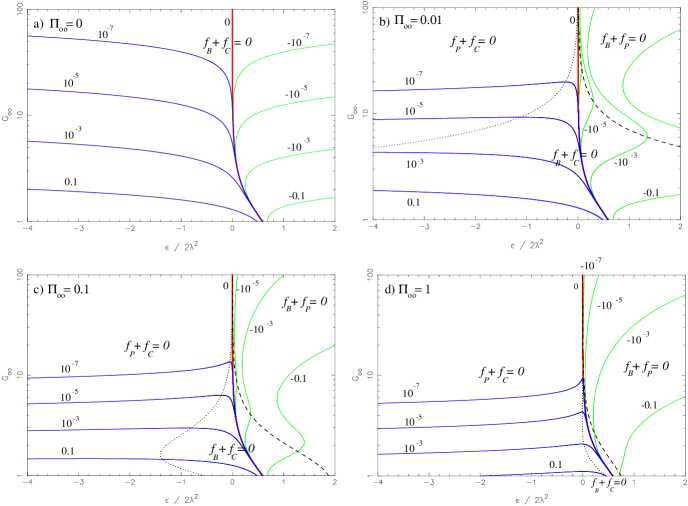
Figure 1: Plots of the asymptotic cylindrical radius normalized to the cylindrical radius at the Alfvén surface $G_{\infty}$ vs. $\epsilon/2\lambda^{2}$ for various values of the final pressure: $\Pi_{\infty}=0$ (panel a), $=0.01$ (panel b), $=0.1$ (panel c) and $=1$ (panel d). Each curve is drawn for a constant value of $\kappa/2\lambda^{2}$ between $-0.1$ and $0.1$ which labels the curve. On the left of the dotted line is the domain of pressure confined jets while on the right of the dashed line is the domain of pressure supported jets and in between is the domain of magnetocentrifugal jets.

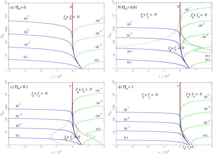
Figure 2: Plots of the asymptotic Alfvén number $M_{\infty}$ vs. $\epsilon/2\lambda^{2}$ for the same values of $\Pi_{\infty}$ and $\kappa/2\lambda^{2}$ as in Fig. 1. On the left of the dotted line is the domain of pressure confined jets while on the right of the dashed line is the domain of pressure supported jets, in between is the domain of magnetocentrifugal jets (except for a small overlap around the dashed line of panel b).

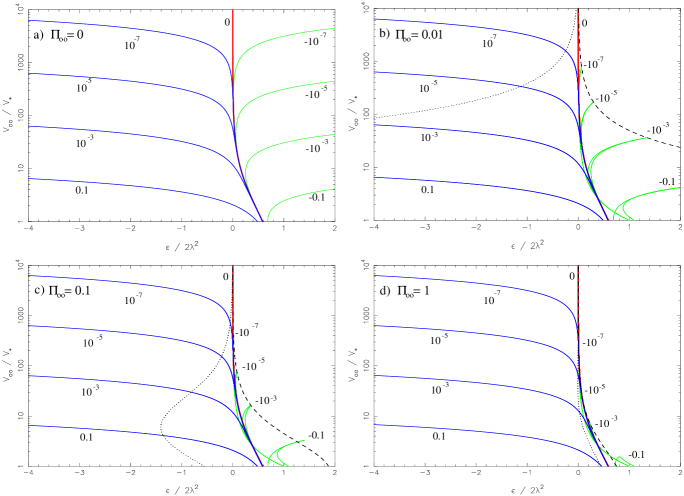
Figure 3: Plots of the asymptotic axial velocity normalized to the polar Alfvén velocity $V_{\infty}/V_{*}$ vs. $\epsilon/2\lambda^{2}$ for the same values of $\Pi_{\infty}$ and $\kappa/2\lambda^{2}$ as in Fig. 1. The domain of pressure confined jets is clearly on the left side of the dotted line and the magnetocentrifugal one in between the dotted and dashed line. However the pressure supported domain overlaps the magnetocentrifugal one.

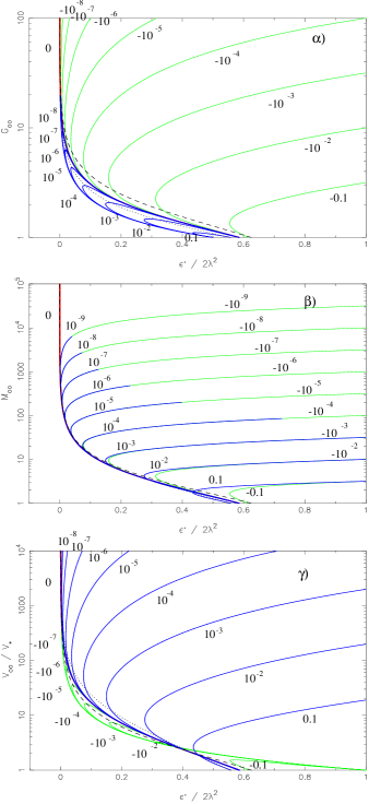
Figure 4: Plots of the asymptotic cylindrical radius (panel $\alpha$), Alfvén number (panel $\beta$) and axial velocity (panel $\gamma$) vs. $\epsilon^{\prime}/2\lambda^{2}$. $G_{\infty}$ and $V_{\infty}$ are normalized to the cylindrical radius and the polar Alfvén velocity at the Alfvén surface, respectively. Each curve is drawn for a constant value of $\kappa\Pi_{\infty}/2\lambda^{2}$ (and not $\kappa/2\lambda^{2}$) between $-0.1$ and $0.1$ which labels the curve. Curves labeled with $0$ correspond to all curves of panels (a) in Figs. 1–3, curves labeled with an even power of 10 correspond to curves drawn in panels (c) of Figs. 1–3, while curves labeled with an odd power of 10 correspond to curves drawn in panels (b) and (d) of Figs. 1–3.

We proceed now towards an asymptotic analysis of the equations of motion, in particular in the case of cylindrical collimation.

4.1 Asymptotic equilibrium in cylindrically collimated outflows

When the equilibrium is asymptotically cylindrical $\epsilon^{\prime}>0$ as discussed above. Taking the dominant terms in the $\theta$-component of the momentum equation or, equivalently by expressing force balance across the cylindrical fieldlines, we obtain the condition of MHD equilibrium in the cylindrical radius direction ${\hat{\varpi}}$ expressed by the equation,

$$\vec{f}_{C}+\vec{f}_{B}+\vec{f}_{P}=0\,.$$

In the asymptotic regime, the centrifugal ($\vec{f}_{C}$), magnetic ($\vec{f}_{B}$) and gas pressure gradient ($\vec{f}_{P}$) forces have the familiar expressions,

$$\vec{f}_{C}={\rho V^{2}_{\varphi}\over\varpi}{\hat{\varpi}}\,,$$

$$\vec{f}_{B}=-\left[{\hbox{d}\over\hbox{d}\varpi}\left(B^{2}_{\varphi}\over 8\pi\right)+{B^{2}_{\varphi}\over 4\pi\varpi}\right]{\hat{\varpi}}\,,$$

$$\vec{f}_{P}=-{\hbox{d}P\over\hbox{d}\varpi}{\hat{\varpi}}\,.$$

In our notation, they can be written as,

$$\vec{f}_{C}={\rho_{*}V_{*}^{2}\over r_{*}}{\lambda^{2}\over G^{3}_{\infty}M^{2}_{\infty}}\left({M^{2}_{\infty}-G^{2}_{\infty}\over M^{2}_{\infty}-1}\right)^{2}\sqrt{\alpha}{\hat{\varpi}}\,,$$

$$\vec{f}_{B}=-{\rho_{*}V_{*}^{2}\over r_{*}}{2\lambda^{2}\over G^{3}_{\infty}}\left(G^{2}_{\infty}-1\over M^{2}_{\infty}-1\right)^{2}\sqrt{\alpha}{\hat{\varpi}}\,,$$

$$\vec{f}_{P}=-{\rho_{*}V_{*}^{2}\over r_{*}}{\kappa\Pi_{\infty}\over G_{\infty}}\sqrt{\alpha}{\hat{\varpi}}\,.$$

Note that always the centrifugal force acts outwards while the total magnetic force (pinching plus pressure) inwards. On the other hand, the last term (not appearing in the Paper III study) is the pressure gradient that acts outwards if the flow is overpressured ($\kappa<0$, i.e. the pressure decreases away from the axis). In this case the jet is necessarily magnetically confined but either centrifugally supported or pressure supported. Conversely, the pressure gradient acts inwards if the flow is underpressured ($\kappa>0$, i.e. the pressure increases away from the axis). In this case the flow is centrifugally supported but may be either magnetically confined or pressure confined.

By combining the asymptotic transverse force balance (Eqs. 4.1 - 4.3),

$$-{1\over 2G^{2}_{\infty}M^{2}_{\infty}}\left({M^{2}_{\infty}-G^{2}_{\infty}\over M^{2}_{\infty}-1}\right)^{2}+{1\over G^{2}_{\infty}}\left({G^{2}_{\infty}-1\over M^{2}_{\infty}-1}\right)^{2}$$

$$+{\kappa\over 2\lambda^{2}}{\Pi_{\infty}}=0\,,$$

with the expression of $\epsilon$ calculated at infinity (Eq. 3.11)

$${\epsilon\over 2\lambda^{2}}=-{\kappa\over 2\lambda^{2}}{M^{4}_{\infty}\over G^{4}_{\infty}}+{1\over{(M^{2}_{\infty}-1)^{2}}}\times$$

$$\left[{(M^{2}_{\infty}-G^{2}_{\infty})^{2}\over 2G^{2}_{\infty}}+(G^{2}_{\infty}-1)(M^{2}_{\infty}-1)\right]\,,$$

we obtain the asymptotic jet radius and Alfvén number as functions of the parameters $\epsilon/2\lambda^{2}$, $\kappa/2\lambda^{2}$ and the asymptotic pressure $\Pi_{\infty}$. Plots of the resulting values of $G_{\infty}$, $M_{\infty}$ and the axial terminal speed $V_{\infty}/V_{*}$ vs. $\epsilon/2\lambda^{2}$ for four representative values of $\Pi_{\infty}$ (0, 0.01, 0.1 and 1) are shown in Figs. 1–3. In each of these panels the values of $G_{\infty}$, $M_{\infty}$ and $V_{\infty}$ are plotted for a range of values of the pressure parameter $\kappa/2\lambda^{2}$ between $-0.1$ and $0.1$ which label the curves.

In parallel we also plot (Fig. 4) $G_{\infty}$, $M_{\infty}$ and $V_{\infty}/V_{*}$ vs. $\epsilon^{\prime}/2\lambda^{2}$ using Eq. (3.17) to determine $\epsilon^{\prime}/2\lambda^{2}$. Note that (see Eqs. 4.4) $G_{\infty}$, $M_{\infty}$ and $V_{\infty}/V_{*}$ depend only on $\epsilon^{\prime}/2\lambda^{2}$ and $\kappa\Pi_{\infty}/2\lambda^{2}$. So conversely to Figs. 1–3 where each curve is drawn for given values of $\Pi_{\infty}$ and $\kappa/2\lambda^{2}$ independently, the curves of Fig. 4 are drawn for a constant and unique value of $\kappa\Pi_{\infty}/2\lambda^{2}$ which labels the curve. In Fig. 5 we make an explicit comparison of the plot $G_{\infty}$ vs. $\epsilon/2\lambda^{2}$ of Fig. 1a and the corresponding curve $G_{\infty}(\epsilon^{\prime}/2\lambda^{2})$ for $\kappa\Pi_{\infty}/2\lambda^{2}=0$.

In these plots we may find three different regimes for the asymptotic state of the collimated outflow according to the various confinement and support conditions across the jet.

4.2 Magnetocentrifugal jets with $f_{C}=|f_{B}|$

This is the case when the pressure gradient is exactly zero $f_{P}=0$ i.e., the pinching magnetic force is balanced by the inertial (centrifugal) force alone. The two following cases correspond to this situation.

4.2.1 Spherically symmetric pressure, $\kappa=0$

The pressure is everywhere spherically symmetric. The terminal value of the pressure does not affect the asymptotic equilibrium in the jet, regardless if it is finite ($\Pi_{\infty}\neq 0$) or zero ($\Pi_{\infty}=0$). This situation corresponds to the thick solid curve labeled 0 in Figs. 1–3. This special and simplest case has been already discussed in detail in Paper III where it was found that the outflow collimates into a cylindrical jet only for $\epsilon>0$, because in this case $\epsilon=\epsilon^{\prime}$. For a given $\lambda$, if the flow remains superAlfvénic, $M_{\infty}>1$, an upper limit exists for $\epsilon$. For $\epsilon/2\lambda^{2}\longrightarrow\epsilon_{\rm max}/2\lambda^{2}=(2-\sqrt{2})\approx 0.586$, then $M_{\infty}\longrightarrow 1$ and $G^{2}_{\infty}\longrightarrow 1$ (see Figs. 1 and 2). As $\epsilon$ decreases from $\epsilon_{\rm max}$ the jet’s radius, Alfvén number and terminal speed increase. Finally, as $\epsilon\longrightarrow 0$, $G_{\infty}\longrightarrow\infty$, $M_{\infty}\longrightarrow\infty$ and $V_{\infty}\longrightarrow\infty$. The streamlines become conical and the asymptotic speed diverges. No collimated solutions at all exist for $\epsilon<0$, as is evident from the plots.

4.2.2 Vanishing asymptotic pressure, $\Pi_{\infty}=0$

The asymptotic gas pressure is zero such that we have again $f_{P}=0$, even though $\kappa\neq 0$. This is the case shown in Figs. 1a–3a where, besides the collimated solutions of the Paper III case obtained for $\epsilon>0$ and $\kappa=0$ (the thick solid branch), we have now collimated solutions for practically all values of $\epsilon$, $-\infty<\epsilon<+\infty$. More specifically, collimated solutions are found to the left of the thick solid branch for $\kappa>0$ (mainly for $\epsilon<0$) and to the right of the thick solid branch for $\kappa<0$.

All branches converge for positive $\epsilon$ and small $G_{\infty}$ towards the thick solid line. Physically this corresponds to the limit (see Eqs. 4.4b and 3.17) where $\kappa V^{2}_{\infty}/V^{2}_{*}$ becomes negligible and the magnetocentrifugal collimation arises because of the central EMR as in Paper III ($\epsilon^{\prime}\approx\epsilon$). Thus we can compare Figs. 1a–3a to the related curve $\kappa\Pi_{\infty}/2\lambda^{2}=0$ of Figs. 4 and 5b. As $\Pi_{\infty}=0$, $G_{\infty}$, $M_{\infty}$ and $V_{\infty}/V_{*}$ depend only on $\epsilon^{\prime}$, namely

$$M_{\infty}=\sqrt{2}\left[{2\lambda^{2}\over\epsilon^{\prime}}-1\right]\,,\quad G^{2}_{\infty}={4\lambda^{2}\over\epsilon^{\prime}}\left[{2\lambda^{2}/\epsilon^{\prime}}-1\over{4\lambda^{2}/\epsilon^{\prime}}-1\right]\,.$$

This is identical to Eqs. (5.13) and (5.14) in Paper III with $\epsilon^{\prime}$ replacing $\epsilon$.

However, even with $\epsilon<0$, we have $\epsilon^{\prime}>0$ provided that $\kappa V^{2}_{\infty}/V^{2}_{*}$ is larger than $|\epsilon|$. In fact with $M_{\infty}>G_{\infty}$ ($\Leftrightarrow V_{\infty}>V_{*}$), the ratio ${V^{2}_{\infty}/V^{2}_{*}}$ is large and positive and can compensate all negative values of $\epsilon$ even for small values of $\kappa$. In this way, even as $\epsilon\longrightarrow-\infty$, $\epsilon^{\prime}>0$ and collimated solutions are obtained, albeit with rather large radii $G_{\infty}$. In physical terms, this corresponds to a situation where the central source is an IMR and cannot collimate the flow through magnetic processes alone. Nevertheless, first it is possible that the conversion of thermal energy into kinetic energy is very efficient ${M^{4}_{\infty}/G^{4}_{\infty}}\gg 1$. Second, it can be more efficient on a non polar streamline than on the polar one if there is more thermal energy in the nonpolar streamlines than in the polar one ($\kappa>0$). In this case then as the flow expands it will build up pressure gradients that will force the lines to bent towards the axis. Once the thermal energy is converted into kinetic energy and the pressure is becoming negligible the magnetocentrifugal forces will dominate. However the collimation is obviously less efficient (larger $G_{\infty}$) than that produced by a central EMR (Fig. 1a). Therefore, this excess of thermal energy induces the collimated character of the solution through the energy integral, even though the corresponding pressure force $f_{P}$ does not enter directly into the asymptotic force balance condition. The term “magnetocentrifugal confinement” can be used for all $(\epsilon/2\lambda^{2},\kappa/2\lambda^{2})$ values of Figs. 1a–3a.

For $\kappa<0$, in order to keep $\epsilon^{\prime}>0$, larger values of $\epsilon$ are required, in comparison to the simple $\kappa=0$ case. In physical terms this is so because now there is a deficit of thermal energy along the nonpolar streamlines in comparison to the polar one and therefore the star has to be a more efficient magnetic rotator (larger values of $\epsilon>0$) in order to have a collimated outflow. This trend is shown by the grey branches to the right of the thick solid branch corresponding to $\kappa=0$ (Figs. 1a–3a).

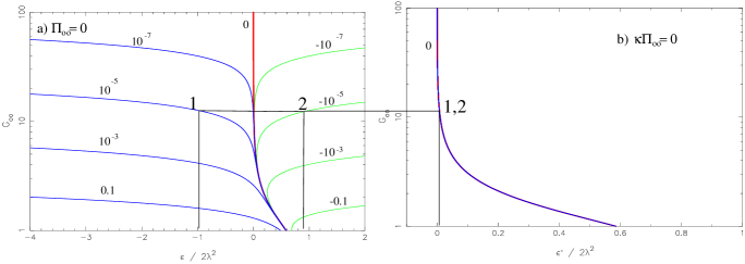
Figure 5: Comparison of the plots of the asymptotic cylindrical radius normalized to the cylindrical radius at the Alfvén surface $G_{\infty}$ vs. $\epsilon/2\lambda^{2}$ (panel a) and vs. $\epsilon^{\prime}/2\lambda^{2}$ (panel b). Each curves on the left panel (a) are drawn for a constant value of $\kappa/2\lambda^{2}$ which labels the curve. All these curves correspond to a unique curve on the right panel (b) because they all have the same value $\kappa\Pi_{\infty}/2\lambda^{2}=0$. We see that for each value of $\epsilon^{\prime}/2\lambda^{2}$, we can find the same value for $G_{\infty}$ for a pair of values of $\epsilon/2\lambda^{2}$ and $\kappa/2\lambda^{2}$ which have approximately the same magnitude but opposite sign (points 1 and 2).

Note that for $\kappa>0$, for each value of $\epsilon/2\lambda^{2}$ there exists a single value of $G_{\infty}$, $M_{\infty}$ and $V_{\infty}$. On the other hand for $\kappa<0$, more values of $G_{\infty}$, $M_{\infty}$ and $V_{\infty}$ correspond to the same value of $\epsilon$. However the lower value of $G_{\infty}$ is practically coincident with that of $\kappa=0$: in other words, thermal decollimation is negligible, similarly to the case $\kappa=0$ and $\epsilon^{\prime}\approx\epsilon$. The upper values of the branches correspond to efficient conversion of thermal energy into polar acceleration but with a deficit along non polar lines. It induces a more drastic conversion of the Poynting flux into acceleration along non polar lines thus reducing the efficiency of the collimation (Fig. 1, $G_{\infty}$ larger) despite the fact that the central object is an EMR ($\epsilon>0$).

This is illustrated in Fig. 5 where the asymptotic cylindrical radius $G_{\infty}$ is plotted versus $\epsilon/2\lambda^{2}$ and $\epsilon^{\prime}/2\lambda^{2}$ for various $\kappa/2\lambda^{2}$ and $\Pi_{\infty}=0$. The higher value of $G_{\infty}$ corresponds to a higher conversion of thermal energy that decollimates the wind which is balanced by a strong EMR as we explained. For some value of $\epsilon^{\prime}=\epsilon+\kappa{V_{\infty}^{2}/V^{2}_{*}}$, we can find the same value for $G_{\infty}$ for a pair of values of $\epsilon$ and $\kappa$ which have approximately the same magnitude but opposite sign (see Fig. 5, points 1 and 2).

Note that a situation with $\Pi_{\infty}=0$ corresponds to very specific initial conditions of integration that may not be easily fulfilled for a cylindrically collimated flow. In particular $\Pi_{\infty}=0$ would imply $T_{\infty}=0$ and the existence of some efficient cooling.

4.3 Magnetocentrifugal jets with $f_{C}\approx|f_{B}|$

In addition to the case wherein $\Pi_{\infty}=0$ shown in Figs. 1a–3a, where we have an exact magnetocentrifugal equilibrium everywhere, approximate magnetocentrifugal equilibrium conditions also exist for $\Pi_{\infty}\neq 0$. This is shown in Figs. 1b–d, 2b–d, 3b–d and 4, in a region adjacent to the thick solid curve obtained for $\kappa=0$, between the dashed and the dotted lines.

4.3.1 Underpressured jets, $\kappa>0$

Following a branch of $\kappa>0$ on the left side of the limiting curve $\kappa=0$, we see from the plots of the various forces shown in Fig. 6, that as $\epsilon/2\lambda^{2}$ decreases the magnetic confinement of the jet is replaced by a pressure confinement, as expected. This transition from magnetic confinement to pressure confinement can be found by writing $f_{P}=f_{B}$, or equivalently, $|f_{B}|=f_{C}/2$ which gives

$$G_{\infty}^{2}={M_{\infty}^{2}+2M_{\infty}\over 1+2M_{\infty}}\,.$$

By inserting this relation in Eq. (4.4b), we obtain the dotted line of Figs. 1–4. Thus, for some finite value of $\Pi_{\infty}$, for each positive value of $\kappa/2\lambda^{2}$, there exists a single value of $\epsilon/2\lambda^{2}=\epsilon_{P-B}/2\lambda^{2}$ located on the dotted line where there is an equal contribution by the magnetic and gas pressure forces in confining the jet against the outwards inertial (centrifugal) force. On the left side of the dotted line the jet enters the regime of gas pressure confinement, which we shall further discuss in the next subsection.

We note that the limit between the two confinement regimes is close to the maximum of the cylindrical radius $G_{\infty}$ as a function of $\epsilon/2\lambda^{2}$, for each value of $\kappa/2\lambda^{2}$ (Figs. 1b–1d). The limit is also very close to the minimum value that $\epsilon^{\prime}/2\lambda^{2}$ can achieve for a given value of $\kappa/2\lambda^{2}$ (Fig. 4$\alpha$, thick solid lines). On the other hand, $M_{\infty}$ and $V_{\infty}$ are monotonic functions of $\epsilon/2\lambda^{2}$.

This maximum radius of the jet can be calculated formally from Eq. (4.4b),

$$G_{\infty}^{2}=M_{\infty}^{2}\,{2M_{\infty}^{2}+\sqrt{4M_{\infty}^{6}-11M_{\infty}^{4}+10M_{\infty}^{2}-3}\over 4M_{\infty}^{4}-3M_{\infty}^{2}+1}\,,$$

which can be combined with Eq. (4.4a) to give the radius as a function of the parameters $\epsilon/2\lambda^{2}$, $\kappa/2\lambda^{2}$ and $\Pi_{\infty}$.

It is interesting to note that, in the limit of large Alfvén numbers ($M_{\infty}\gg 1$) the two values of $G_{\infty}$ given by Eqs. (4.6) and (4.7) coincide and to first order we have

$$G_{\infty}^{2}\approx{M_{\infty}\over 2}\approx\left(\lambda^{2}\over 8\kappa\Pi_{\infty}\right)^{1/3}\,.$$

Then the asymptotic velocity along the polar axis is (see Eq. 3.4c)

$${V_{\infty}\over V_{*}}\approx\left(8\lambda^{2}\over\kappa\Pi_{\infty}\right)^{1/3}\,,\quad\lambda={\Omega({\rm pole})r_{*}\over V_{*}}\,.$$

The terminal speed has the same dependence on the dimensionless rotational speed $\lambda$ with Michel’s minimum energy solution for cold magnetic rotators wherein $V_{\infty}/V_{*}=\lambda^{2/3}$. In the present case however, the asymptotic speed is enhanced by the factor $[8/\kappa\Pi_{\infty}]^{1/3}$. For small values of $\kappa$ and $\Pi_{\infty}$ of the order of 1, this is indeed a rather large enhancement. This increased terminal speed simply reflects the transformation to asymptotic kinetic energy of the enthalpy and added thermal energies. Note also that when $\Pi_{\infty}\longrightarrow 0$, $V_{\infty}\longrightarrow\infty$. This is expected and the situation is similar to the radial outflow studied in Tsinganos & Trussoni (1991) where the terminal speed is

$${V_{\infty}\over V_{*}}\approx 6\left(\lambda^{2}\ln R\right)^{1/3}\,.$$

4.3.2 Overpressured jets, $\kappa<0$

The regime of magnetocentrifugal equilibrium extends also to the right of the thick solid line $\kappa=0$ and up to the dashed line in Figs. 1 and 2. Beyond this line the jet enters in the regime of gas pressure support which we shall discuss later.

Figure 6: Asymptotic transversal forces vs. $\epsilon/2\lambda^{2}$ for a positive value of $\kappa$, $\kappa/2\lambda^{2}=0.001$: centrifugal force ($f_{C}$, solid line), magnetic force ($f_{B}$, dashed line) and pressure gradient ($f_{P}$, dotted line). The asymptotic pressure is $\Pi_{\infty}=0$ (panel a), $=0.01$ (panel b), $=0.1$ (panel c) and $=1$ (panel d). The bullet marks the value of the centrifugal force $f_{C}$ for which $f_{P}=f_{B}$.

Figure 7: The same as Fig. 6, for a negative value of $\kappa$, $\kappa/2\lambda^{2}=-0.001$ but the magnetic force ($f_{B}$) corresponds to the solid line, the centrifugal force ($f_{C}$) to the dashed one and the pressure gradient ($f_{P}$) to the dotted one. The bullet marks the value of the magnetic force $f_{B}$ for which $f_{P}=f_{C}$.

Following a branch of $\kappa<0$ on the right side of the limiting curve $\kappa=0$, Fig. 7 illustrates how the centrifugal force decreases and is progressively dominated by the pressure gradient. The transition from centrifugal support to pressure support can be estimated by writing $f_{P}=f_{C}$, or equivalently, $|f_{C}|=f_{B}/2$ which gives

$$G_{\infty}^{2}=M_{\infty}\,.$$

This relation can be combined with Eq. (4.4b) to give the dashed limiting line (Figs. 1–4) where $\epsilon/2\lambda^{2}=\epsilon_{P-C}/2\lambda^{2}$. For $G_{\infty}\gg 1$ this limit coincides also approximately with the maximum of the velocity on an assumed $\kappa/2\lambda^{2}$ branch (Fig. 3), given by

$${V_{\infty}\over V_{*}}\biggr{|}_{\rm max}={1\over{2G^{2}_{\infty}}}\times\left[G_{\infty}^{4}-4G_{\infty}^{2}+5\right.$$

$$\left.+\sqrt{G_{\infty}^{8}-8G_{\infty}^{6}+26G_{\infty}^{4}-40G_{\infty}^{2}+21}\right]\,,$$

(in this domain the curves of the jet radius $G_{\infty}$ and Alfvén number $M_{\infty}$ are monotonic with $\epsilon/2\lambda^{2}$). We remark that the curve of maximum velocity (d̃ashed line) also corresponds to the minimum value of $\epsilon^{\prime}/2\lambda^{2}$ for a given value of $\kappa/2\lambda^{2}$, in the limit of large Alfvén number (see Fig. 4$\gamma$, thin solid lines).

For $G_{\infty}\gg 1$ we have from Eqs. (4.10):

$${V_{\infty}\over V_{*}}\biggr{|}_{\rm Max}\approx\left({{2\lambda^{2}}\over{|\kappa|\Pi_{\infty}}}\right)^{1/3}\,,$$

i.e. the same scaling law with $|\kappa|/2\lambda^{2}$ and $\Pi_{\infty}$ holds for the maximum velocity as for the asymptotic velocity at maximum radius for $\kappa>0$ (Eq. 4.8b).

4.3.3 $\epsilon_{P-B}<\epsilon<\epsilon_{P-C}$

In the intermediate region bounded by the two curves $\epsilon_{P-B}$ and $\epsilon_{P-C}$, the jet is magnetocentrifugal. Solutions very close to the thick solid line correspond to an efficient collimation by the EMR with negligible thermal contributions, as we already discussed. For small values of $\Pi_{\infty}$ (e.g., Figs. 1b–3b) this area is surrounded by solutions with important thermal energy conversion but small asymptotic pressure gradients similar to the extended branches of Figs. 1a–3a. However, for larger $\Pi_{\infty}$ the jets can be in magnetocentrifugal regime only for a narrow range of values of $\epsilon/2\lambda^{2}$, around the line $\kappa=0$ (see Figs. 1c–3c and 1d–3d: the region between the dotted and dashed lines shrinks by increasing $\Pi_{\infty}$).

4.4 Pressure confined jets $f_{C}\approx|f_{P}|$

The more negative $\epsilon/2\lambda^{2}$ becomes, the weaker are the magnetic pinching forces (the less efficient is the magnetic rotator). Thus, for $\epsilon<\epsilon_{P-B}$ (left of the dotted line on Figs. 1b–1d, 2b–2d, 3b-3d and 4$\alpha$) the magnetic pinching force has dropped to very small values in comparison to the gas pressure force $f_{P}$, such that now $f_{P}$ alone confines the jet against the inertial force (Fig. 6). The situation is similar to the case of the prescribed streamlines studied in TTS97 ($q>0$, in the upper branch of curves in the right panel of Fig. 1 in this paper).

The asymptotic radius of the jet and its Alfvén number are sensitive to the nature of the asymptotic confinement. They strongly depend on the value of $\Pi_{\infty}$ (e.g., Figs. 1–2). At the same time, the terminal speed $V_{\infty}/V_{*}$ is almost independent of the value of the terminal gas pressure $\Pi_{\infty}$ (e.g., Fig. 3) for strongly negative values of $\epsilon/2\lambda^{2}$. This can be understood from Eq. (4.4b) where we see that in the limit of negative $\epsilon/2\lambda^{2}$ the first term of the right hand side dominates and thus the square of the terminal speed is roughly given by the ratio $|\epsilon|/\kappa$.

For $\epsilon\ll\epsilon_{P-B}$ we are basically entering the hydrodynamic regime studied in Paper I. In the limit of $\epsilon\rightarrow-\infty$ and finite asymptotic pressure, the jet is strongly pressure confined such that $G_{\infty}(\epsilon\rightarrow-\infty)<1$ (cf. Figs. 1b–1d, 2b–2d, 3b–3d), i.e., the solution becomes unphysical. As in Paper I we find that the most physically interesting hydrodynamic solution is obtained for vanishing terminal pressure with conical asymptotics wherein $G_{\infty}(\epsilon\rightarrow-\infty)\rightarrow\infty$ (e.g., Fig. 1a – 3a).

We may see the hydrodynamical limit as the most extreme one. Nevertheless, even with a non vanishing magnetic field, we note that the more efficient is the pressure confinement of the jet (the more negative is $\epsilon/2\lambda^{2}$) the larger is the gap between the value of the jet radius $G_{\infty}$ obtained for $\Pi_{\infty}=0$ and the one obtained for $\Pi_{\infty}\mathbin{\raise 2.0pt\hbox{$>$}\hskip-9.0pt\lower 4.0pt\hbox{$\sim$}}0$ (Figs. 1a and 1b), for a given value of $\kappa/2\lambda^{2}$. The difference is even larger when $\kappa/2\lambda^{2}$ takes small values. In such a case the magnetocentrifugal forces are very weak (Fig. 6) and the equilibrium is very sensitive to small changes in the pressure gradient.

4.5 Pressure Supported Jets with $f_{P}\approx|f_{B}|$

This last case occurs when the centrifugal forces are negligible i.e., the jet is confined by magnetic forces and is supported by the gas pressure gradient (for $\epsilon>\epsilon_{P-C}$, right side of dashed line, but only in Figs. 1b–d, 2b–d and 4$\alpha$).

Now the inertial force has dropped to very small values in comparison to the gas pressure gradient force such that $f_{P}$ alone supports the jet against the magnetic pinching force (see Fig. 7). In this domain, for a given value of $\kappa/2\lambda^{2}$, the centrifugal force exactly vanishes for $M_{\infty}=G_{\infty}$ (Eq. 4.3a), when $V_{\infty}=V_{*}$. It simply states that a jet with zero asymptotic centrifugal force has no net acceleration between the Alfvén surface and infinity. At this particular point $\epsilon/2\lambda^{2}=(\epsilon/2\lambda^{2})_{0}$ where the asymptotic centrifugal force is exactly zero and $V_{\infty}=V_{\star}$, we obtain from Eq. (4.4b),

$$\left(\epsilon\over 2\lambda^{2}\right)_{0}+{\kappa\over 2\lambda^{2}}=1\,.$$

Since $\kappa/2\lambda^{2}$ is usually rather small, it follows that $(\epsilon/2\lambda^{2})_{0}\approx 1$. There, we can say that the jet is exactly supported by the pressure gas gradient alone. If we start at $(\epsilon/2\lambda^{2})_{0}$ and move toward larger values of $\epsilon/2\lambda^{2}$, along the branch $\kappa/2\lambda^{2}=const<0$, $M_{\infty}$ and $G_{\infty}$ increase, rotation changes sign (See Eq. A.3f) and the asymptotic velocity is less than the velocity at the Alfvén point (Fig. 3) which means that the outflow is decelerated though it remains superAlfvénic (we do not consider in the present analysis “breeze” solutions that are always subAlfvénic).

By starting at $(\epsilon/2\lambda^{2})_{0}$ and moving in the opposite direction toward smaller values of $M_{\infty}$ and $G_{\infty}$ along the branch $\kappa/2\lambda^{2}=const<0$, the inertial force remains negligible in comparison to the gas pressure gradient, up to the dashed line wherein we enter the magnetocentrifugal domain.

5 Oscillations in the jet’s width

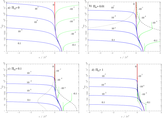
Figure 8: Plots of the wavelength of the oscillations $\Lambda_{\rm osc.}$ in units of $r_{*}/\lambda$ vs. $\epsilon/2\lambda^{2}$ for the same values of $\Pi_{\infty}$ and $\kappa/2\lambda^{2}$ as in Figs. 1–3. On the left of the dotted line is the domain of pressure confined jets while on the right of the dashed line is the domain of pressure supported jets and in between is the domain of magnetocentrifugal jets.

The previous analysis giving the asymptotic equilibrium for confined jets can be pushed one step further to the first order terms in the bending of the lines (Paper III, Vlahakis & Tsinganos 1997, henceforth VT97). We also assume there that the jet becomes asymptotically cylindrical. An expansion of $G$ and $M$ can be made then to get an idea of the fluctuations that exist far from the region of the initial acceleration of the wind,

$$G^{2}=G^{2}_{\infty}(1+\vartheta)\,,$$

$$M^{2}=M^{2}_{\infty}(1+\mu)\,,$$

where $\vartheta,\,\mu\ll 1$. Conversely to Paper III, we must also expand the pressure as

$$\Pi=\Pi_{\infty}(1+p)\,.$$

Thus we obtain the harmonic oscillator equation for the perturbed jet radius (see Appendix C for details):

$$\ddot{\vartheta}+\left(2\pi r_{*}/\Lambda_{\rm osc.}\right)^{2}\vartheta=0\,,$$

where $\Lambda_{\rm osc.}$ is the wavelength of the oscillations. We can write the wavelength of the oscillations in the form of VT97, Eq. (28), namely

$$\left(2\pi r_{*}\over\Lambda_{\rm osc.}\right)^{2}={2\lambda^{2}\over(1-M_{\infty}^{2})^{2}}\left[2+{\mu\over\vartheta}{(2M_{\infty}^{2}-1)G_{\infty}^{4}-M_{\infty}^{4}\over M^{2}_{\infty}(1-M_{\infty}^{2})}\right]$$

with in the present case

$${\mu\over\vartheta}={\displaystyle{\kappa\over\lambda^{2}}-{G_{\infty}^{2}\over M_{\infty}^{4}}{M_{\infty}^{4}+G_{\infty}^{4}(1-2M_{\infty}^{2})\over 2(1-M_{\infty}^{2})^{2}}\over\displaystyle{\kappa\over\lambda^{2}}-G^{2}_{\infty}{(1-G_{\infty}^{2})^{2}\over(1-M_{\infty}^{2})^{3}}}\,.$$

Plots of the asymptotic wavelength $\Lambda_{\rm osc.}$ vs. $\epsilon/2\lambda^{2}$ for four representative values of $\Pi_{\infty}$ are shown in Fig. 8. In each of these plots, the values of $\Lambda_{\rm osc.}$ are plotted for the range of the pressure parameter $\kappa/2\lambda^{2}$ as in Figs. 1 to 3.

In the domain of magnetocentrifugal jets the wavelength behaviour is very similar to the one found in Paper III as expected. In the case of $\kappa=0$ studied in Paper III, Eq. (5.4) takes the very simple form (Vlahakis, private communication)

$$\left(2\pi r_{*}/\Lambda_{\rm osc.}\right)^{2}={4\lambda^{2}\over M_{\infty}^{2}(M_{\infty}^{2}-1)}$$

In the domain of pressure confined jets (which corresponds always to underpressured jets, $\kappa>0$), the wavelength of the oscillations behaves like the Alfvén number despite of the decrease of the cylindrical radius. In particular, as the rotator slows down ($\epsilon/2\lambda^{2}$ decreasing) the wavelength increases very slowly. Nevertheless in the limit $\epsilon/2\lambda^{2}\rightarrow-\infty$ where we enter the hydrodynamic regime the wavelength must eventually diverge. The similarity of the curves of Figs. 2 and 8 on logarithmic scales, which reflects the similar behaviour of $M_{\infty}$ and $\Lambda_{\rm osc}$, can be easily understood in the limit of large values of $M_{\infty}$ and $V_{\infty}/V_{*}$. In this limit – which is by the way expected to be the case for most observed jets – we get that the wavelength is just proportional to the square of the Alfvén number, $\Lambda_{\rm osc}\sim M^{2}_{\infty}\,.$ Note also that, if the wavelength of the oscillations can be related to the observed morphology of the jets, we may have here an indirect estimate of the magnitude of the poloidal Alfvén number.

For overpressured jets ($\kappa<0$), the behaviour of $\Lambda_{\rm osc.}$ is similarly following the increase of the Alfvén number as the pressure becomes more important, but as it enters the domain of pressure supported jets after the maximum velocity, the oscillations disappear. In fact in this last case we can see that the pressure gradient supporting the jet cannot restore equilibrium against the confining magnetic pinch. This could imply that the solutions of this class are unstable.

We must notice finally that oscillations in collimated winds are quite a general result, not restricted to our class of meridional self-similar solutions. In fact oscillating structures have been found not only in other self-similar flows (Chan & Henriksen 1980, Bacciotti & Chiuderi 1992, Del Zanna & Chiuderi 1996, Contopoulos & Lovelace 1994, Contopoulos 1995, VT98), but also in more general analyses of axisymmetric outflows (see e.g. Pelletier & Pudritz 1992).

6 Asymptotic equilibrium for non collimated flows

6.1 Existence of asymptotically non collimated flows

If the flow is not cylindrical asymptotically, then $F_{\infty}$ must take a value in the interval $0\leq F_{\infty}<2$, with $F_{\infty}=0$ corresponding to conical asymptotics. Assuming that this value of $F_{\infty}$ and the corresponding shape may be achieved rather slowly, at large distances $R$ from the central object the analytic expression of $F(R)$ can be written as

$$F(R\rightarrow\infty)=F_{\infty}+{c\over\ln R}+\sum_{n=1}^{n\rightarrow\infty}{c_{n}\over R^{n}}\,,$$

where $c$ and $c_{n}$ are constants. As $R\longrightarrow\infty$ the dominant term is the logarithmic one and thus we may keep only this term in the expansion, such that from Eq. (2.6) and (3.4c) we obtain

$$G^{2}(R\rightarrow\infty)={R^{2-F_{\infty}}\over f_{\infty}\ln^{c}(R)}\,,$$

$$M^{2}(R\rightarrow\infty)={R^{2-F_{\infty}}\over f_{\infty}\ln^{c}(R)}{V_{\infty}\over V_{*}}\,,$$

where $f_{\infty}$ is a constant (TTS97, Paper III). By substituting these expressions in the definition of the integral $\epsilon$ of Eq. (3.11) and keeping the dominant terms we get

$${\epsilon\over 2\lambda^{2}}=-{1\over 2\lambda^{2}}{V_{\infty}^{2}\over V_{*}^{2}}\left[\kappa+{1-F_{\infty}^{2}/4\over R^{F_{\infty}}f_{\infty}\ln^{c}(R)}\right]+{V_{*}\over V_{\infty}}$$

$$+{f_{\infty}\ln^{c}(R)\over 2R^{2-F_{\infty}}}\left(1-{V_{\star}\over V_{\infty}}\right)^{2}\,.$$

Assuming $\kappa\neq 0$, Eq. (6.3) shows clearly a rather general result: a diverging asymptotic velocity is inconsistent with the constancy of $\epsilon$. The cylindrical radius and Alfvén number may be unbounded, but the terminal flow speed cannot, no matter what is the exact value of $F_{\infty}$. This is also in agreement with the fact that the fraction of the heating term converted to kinetic energy and $\propto\kappa$ cannot diverge (see Sec. 3.1).

Further insight in the general behaviour of the asymptotics can be gained by considering the dominant terms in the transverse momentum equation which gives a relation for the pressure (see Eq. A.4c in Appendix A),

$$-{\kappa\Pi(R\rightarrow\infty)\over 2\lambda^{2}}=f_{\infty}{V_{*}^{2}\over V_{\infty}^{2}}{\ln^{c}(R)\over R^{2-F_{\infty}}}\,.$$

The first conclusion from this relation is that the asymptotic pressure must vanish because the r.h.s. term (due to the magnetocentrifugal terms) always vanishes for non cylindrically collimated outflows.

A second conclusion is that, independently of the value of $\epsilon$, underpressured flows ($\kappa>0$) must be cylindrically collimated, as found in Sec. 4. This can be explained taking into account that, when the streamlines try to expand, then pinching by both magnetic forces and pressure gradient will dominate over all other forces (Eq. 6.4). To maintain the forces equilibrium a strong bending of the lines towards the axis is required, $R{\hbox{d}F/\hbox{d}R}>0$, such that the system must relax towards a collimated configuration. Then only overpressured outflows ($\kappa<0$) may be non collimated.

6.2 Asymptotically paraboloidal or radial overpressured flows

Assuming $\kappa<0$, we discuss separately the case of paraboloidal ($F_{\infty}>0$) and radial asymptotics ($F_{\infty}=0$).

6.2.1 Paraboloidal asymptotics, $F_{\infty}>0$

Independently on the value of $c$, Eq. (6.3) further simplifies as follows

$${\epsilon\over 2\lambda^{2}}=+{|\kappa|\over 2\lambda^{2}}{V_{\infty}^{2}\over V_{*}^{2}}+{V_{*}\over V_{\infty}}\,,$$

which implies that paraboloidal shapes can exist only for $\epsilon>0$. In other words, only overpressured outflows from an efficient magnetic rotator may eventually achieve a paraboloidal shape. This can be physically understood because such a structure implies some collimation that can be achieved only through magnetic forces in the present case.

We remark that in the case $\kappa=\epsilon=0$ Eq. (6.5) can be fulfilled only for diverging asymptotic velocity (Paper III). However, as we have seen before, such a case would require an infinite heating rate, so that such kind of solutions should be considered as unphysical.

6.2.2 Radial asymptotics, $F_{\infty}=0$

If $c\neq 0$, Eq. (6.5) and the previous remarks still hold. For $c=0$, Eq. (6.3) becomes

$${\epsilon\over 2\lambda^{2}}={1\over 2\lambda^{2}}{V_{\infty}^{2}\over V_{*}^{2}}\left(|\kappa|-{1\over f_{\infty}}\right)+{V_{*}\over V_{\infty}}\,,$$

and radial asymptotics can exist a priori for both negative and positive values of $\epsilon$.

This simple analysis shows that overpressured flows ($\kappa<0$) can attain only radial streamlines if they are IMR ($\epsilon<0$), while they can have cylindrical, paraboloidal or radial asymptotics if they are associated with an EMR ($\epsilon>0$).

We point out finally a common feature for winds with parabolic or radial asymptotics. From Eq. (6.4) we see that temperature goes to a constant value along each fieldline

$$T(R\rightarrow\infty,\alpha)\propto{P\over\rho}={1\over 2}V_{*}^{2}{1+\kappa\alpha\over 1+\delta\alpha}\left(-{2\lambda^{2}\over\kappa}\right){V_{*}\over V_{\infty}}\,,$$

i.e. all uncollimated solutions are isothermal asymptotically. This is consistent with the results of Tsinganos & Trussoni (1991), who analyzed solutions with prescribed radial streamlines [$F(R)=0$]. More in general, we can expect that in non collimated outflows some heating is always necessary in the asymptotic regions. Conversely in a cylindrical jet, where the pressure and density are constant, the temperature is also constant but the heating rate in the flow vanishes (Eq. 3.1b,c).

7 Discussion and astrophysical implications

7.1 Summary of the main results

We have presented here the asymptotic properties of superAlfvénic outflows which are self-similar in the meridional direction. The terminal Alfvén number, $M_{\infty}$, the dimensionless asymptotic radius of the jet, $G_{\infty}$ and velocity, $V_{\infty}/V_{*}$ depend only on three parameters (see Eqs. 4.4). Besides the terminal pressure $\Pi_{\infty}$, the two other crucial parameters are:

$\bullet$ $\kappa/2\lambda^{2}$, connecting the radial and longitudinal components of the gradient of the gas pressure. Thus, the outflow can be either overpressured ($\kappa<0$), or underpressured ($\kappa>0$) with respect to the rotational axis.

$\bullet$ $\epsilon/2\lambda^{2}$, which measures the magnetic contribution to the collimation of the outflow. Thus, we may divide the sources of outflows into two broad classes : Efficient Magnetic Rotators (EMR) corresponding to positive values of $\epsilon$ and a strong magnetic contribution to collimation, and Inefficient Magnetic Rotators (IMR) which have negative $\epsilon$ and can collimate outflows only with the help of the gas pressure.

The absolute criterion for cylindrical collimation is given by the sign of a combination of the two parameters $\kappa/2\lambda^{2}$ and $\epsilon/2\lambda^{2}$. This new parameter

$\bullet$ $\epsilon^{\prime}/2\lambda^{2}$ is related to the variation across the streamlines of the various energy contributions which govern the flow dynamics (magnetocentrifugal, thermal, etc). Thus, a positive value of $\epsilon^{\prime}$ provides cylindrical asymptotics while negative values are required for having uncollimated flows.

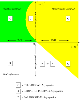
Figure 9: A sketch of the various confinement regimes and asymptotical shapes of the flow in the plane [$\kappa/2\lambda^{2},\,\epsilon/2\lambda^{2}$]. The pressure confined regime corresponds to the area filled with dark grey while the magnetically confined regime corresponds to the light grey filled area. In the remaining area only uncollimated solutions are found.

Despite this simple criterion, the asymptotic behaviour of the outflow still depends on the value of each parameter taken separately as shown in Fig. 9 [see also Figs. (1–3)].

$\bullet$Underpressured outflows. For $\kappa>0$ the wind always obtains cylindrical asymptotics. The jet is supported by the centrifugal force, while collimation can be provided either by the magnetic pinching or the gas pressure, depending on $\epsilon$ and the value of the asymptotic gas pressure $\Pi_{\infty}$. We repeat however that for IMR the state of asymptotic magnetic confinement can be achieved only through the strong pressure gradients occurring between the base of the flow and infinity. If $\Pi_{\infty}$ does not vanish, the jet radius has a maximum when moving from the magnetic to the thermal regime (by reducing $\epsilon/2\lambda^{2}$).

$\bullet$Overpressured outflows. When $\kappa<0$ the jet can be confined by the magnetic pinch only, and is supported either by the centrifugal force or by the thermal pressure gradient. If $\Pi_{\infty}$ does not vanish, the jet terminal velocity has a maximum when moving from the centrifugal to the thermal regime. Moreover, in overpressured outflows, cylindrical configurations are attained only for values of $\epsilon/2\lambda^{2}$ higher than some threshold depending on the pressure parameters, $\Pi_{\infty}$ and $\kappa$. Below this positive threshold value the outflow reaches conical or paraboloidal asymptotics if $\epsilon>0$ (EMR) or only purely conical asymptotics if $\epsilon<0$ (IMR).

Cylindrical collimation seems to be quite a natural end state for superAlfvénic outflows with non vanishing asymptotic pressure, as also found by other studies based on the radial self-similar approach (Li 1995, 1996, Ferreira 1997, Ostriker 1997), or on the full asymptotic treatment of the MHD equations (Heyvaerts & Norman 1989). However in the present case the collimation can be provided not only by the magnetic pinch, but also by the thermal pressure gradient. This is consistent with our self-similar scenario, suitable to model winds close to their rotational axis, where the thermal effects are essential to drive the outflow. We also point out that our results are consistent with those of TTS97, where again different collimation regimes can be found. Finally, we remark that cylindrically collimated streamlines most of times undergo oscillations with different wavelengths.

7.2 Astrophysical application

As in Paper III and TTS97, the present results could be particularly suitable to model the physical properties of collimated outflows associated with Young Stellar Objects (YSO). However, since here we have analyzed only the asymptotic properties of winds, we will shortly discuss only a simple possible scenario based on the physical difference between EMR and IMR.

Let us consider a rapidly rotating magnetized protostar at the beginning of its evolution. In such conditions this object could be considered as an EMR, with a well collimated, magnetically confined jet. At the same time the pressure inhomogeneity $|\kappa|$ and the asymptotic pressure may take rather high values due to the inhomogeneous and anisotropic environment in which the jet is found. In the early phases of stellar evolution the outflow extracts quite efficiently angular momentum from the protostar, reducing its spinning rate. From the point of view of our model this means that the system moves from the state of an EMR to that of an IMR as it lowers the value of $\epsilon$. Of course the details of the evolution may be more complicated due to the feeding of the wind by the surrounding accretion disk. Nevertheless the net end result should be a decrease of the spinning rate and subsequently of the efficiency of the magnetic rotator (Bouvier et al. 1997).

If the jet is initially underpressured, for example being embedded in a dense molecular cloud, as it approaches the regime of the IMR a gradual widening of its radius is expected. This widening may reach a maximum value, wherein the magnetic and thermal contributions to the confinement are comparable. At this stage it is reasonable to expect a decrease of the asymptotic pressure because of this widening. At the same time, we may have a more homogeneous flow, i.e., effectively a decrease of $\kappa$. Thus, in the subsequent evolution of the central young star, we expect that the jet continues increasing its radius. According to this scenario, we can imagine an evolutionary track of the outflow along the maxima from Figs. 1d to Fig. 1b, wherein there is an equal contribution by the thermal and magnetic forces confining the plasma. In this sequence, the terminal velocity always increases, Figs. 3d to 3b, as $\kappa$ and the asymptotic pressure $\Pi_{\infty}$ get lower and lower values. Finally, the outflow becomes a loosely collimated wind.

In the above scenario, it is essential to have a decrease of $\kappa$ and $\Pi_{\infty}$ during the evolution. Because, otherwise, we see that an IMR ($\epsilon<0$) together with a strongly underpressured plasma (high $\kappa\Pi_{\infty}$) have the result to over collimate the wind with an asymptotic radius comparable to its Alfvén radius. This result would be somehow in contradiction with the observed radii of outflows from YSOs which are expected to be much larger than the Alfvén radius. Instead, we propose that both thermal and magnetic confinement decrease simultaneously during the evolution of the central source.

However, jets from planetary nebulae (PN) may present a totally different situation where the primary source of confinement is a strong pressure gradient, $\kappa\Pi_{\infty}\gg 0$, associated with a source which is a very inefficient magnetic rotator, although with a non zero magnetic field. The terminal radii of jets from PN are indeed observed to be rather small after some huge initial widening (Frank 1998). We also note that our analysis favours a hydrodynamical origin of jets from PN similarly to the GWBB model (cf. Mellema & Frank 1997, Frank 1998) and contrarily to a pure magnetic origin of the refocusing of the wind.

The analysis of overpressured jets is more complex at first glance as different regimes are possible for the same $\epsilon$. Let us first consider that the jet is initially quite narrow, centrifugally supported and originates from an EMR; i.e., it is on the lower branches of the thin grey lines ($\kappa<0$) of Figs. 1–3. As in the previous case, the rotation slows down ($\epsilon$ decreases), the outflow rapidly opens and the velocity rises. However, below a threshold value of $\epsilon/2\lambda^{2}$ the flow becomes uncollimated (see Fig. 9).

If, conversely, at the beginning the jet is pressure supported (i.e., on the upper branches of the dotted lines in Figs. 1b–d, 2b–d), the behaviour is quite ambiguous: a reduction or an increase of the jet radius and velocity critically depends on the initial conditions ($|\kappa|$, asymptotic pressure, jet radius) when the star starts slowing down its rotational rate. Then it is difficult to model the possible evolution of a pressure supported jet. But, as we said previously, the absence of oscillations in this region may indicate that such equilibria are in fact unstable and never attained practically.

It is evident from the above that the possible outflow evolution is critically related to its physical conditions, namely if it is underpressured or overpressured. In which of these regimes the outflow can be found depends on the detailed history of the wind. We remind that the thermodynamic conditions across the jet in its asymptotic regime depend also on the assumed structure of density ($\delta$) and the intensity of the gravitational field ($\nu$). These two parameters do not enter in the present analysis, but are essential for the thermal acceleration of the wind (see Paper III and TTS97). Therefore the next step in the present analysis is to make a careful parametric study of the numerical solutions, solving the set of Eqs. (A.4). This is also demanded in order to make a detailed comparison with observational data and implies that we construct solutions that connect the base of the flow with the superAlfvénic region fulfilling the regularity conditions at the critical points (Sauty et al., in preparation). In particular, it will be crucial to see whether or not all the asymptotic regimes presented here can be attained.

7.3 Future directions of study

The present results have been obtained in the framework of a self-similar treatment of the axisymmetric MHD equations. This implies some ‘a priori’ constraints on the structure of the solutions, that we summarize in the following.

The surfaces with the same Alfvénic number are spherical [$M(R,\theta)\equiv M(R)$], with the velocity vanishing on the equatorial plane. Furthermore the $\theta-$ and $r-$ components of the gradient of the gas pressure are linearly related. These assumptions are not too constraining if we consider our model as suitable to describe the physical properties of the flow around the rotational axis. We remind also that our results are consistent with those found in TTS97, where the two components of $\nabla P$ were unrelated in a wind with prescribed cylindrical asymptotics.

Such limits of the present treatment could anyway be overcome by a different scaling of the physical variables with the colatitude. It has been shown in VT98 that the assumptions of Eqs. (2.3) are just a particular case of a more general class of solutions, with no vanishing velocity on the equator and with a more complex expression for the pressure (another particular case is the one studied in Lima et al. 1996; see also Vlahakis 1998). In such a case the set of the MHD equations lead to a closed system whose treatment does not require any further ‘a priori’ assumption as the relation between the components of the pressure gradient (as in Paper III and in the present study) or the prescription of the streamline shape (as in TT97).

Finally, we point out once more that, contrary to the radial self-similar studies, the role of the thermal structure of the flow, which is related to the details of processes of input/output of heating in the gas, is essential in our model and not only in accelerating the flow but also in constructing its global shape. The problem of the energetic behaviour of astrophysical plasmas in different astrophysical contexts (solar and stellar coronae, YSO, AGN) is however still open.

Appendix A Appendix A

The classical equations of ideal MHD steady flows are

$$\nabla\cdot\vec{B}=\nabla\cdot(\rho\vec{V})=\nabla\times(\vec{V}\times\vec{B})=0\,,$$

$$\rho(\vec{V}\cdot\nabla)\vec{V}-(\vec{B}\cdot\nabla)\vec{B}/4\pi$$

$$=-\nabla(p+B^{2}/8\pi)-{\cal G}{\rho{\cal{M}}\over r^{2}}{\bf e}_{r}\,,$$

$$\rho\vec{V}\cdot\left(\nabla h-{{\nabla P}\over{\rho}}\right)=q\,,$$

where $h$ is the enthalpy of the perfect gas, $q$ is the local volumetric heating rate including true heating and cooling, ${\cal G}$ is the gravitational constant, ${\cal M}$ is the mass of the central object and the other symbols have their usual meaning.

Under the assumption of steady state and axisymmetry, the existence of free integrals as defined in the main text gives the usual forms for the poloidal ($p$) components of the magnetic field $\vec{B}$ and the velocity $\vec{V}$, using spherical ($r,\theta,\varphi$) or cylindrical ($\varpi,\varphi,z$) coordinates (for details see Tsinganos 1982)

$$\vec{B}_{p}={\nabla A\over\varpi}\times{\bf e}_{\varphi}\,,\qquad\vec{V}_{p}={\Psi_{A}\over 4\pi\rho}\vec{B}_{p}\,,$$

while the toroidal components are

$$B_{\varphi}=-{{L(A)\Psi_{A}}\over\varpi}{{1-\varpi^{2}\,\Omega(A)/L(A)}\over{1-M^{2}}}\,,$$

$$V_{\varphi}={L(A)\over\varpi}\,{\varpi^{2}\,\Omega(A)/L(A)-M^{2}\over 1-M^{2}}\,,$$

where $M$ is the poloidal Alfvén Mach number as defined in Eq. (2.1).

Considering our assumptions, Eqs. (2.3), we get that the components of the velocity and magnetic field reduce in our model to

$$B_{r}=B_{*}{1\over G^{2}(R)}\cos\theta\,,$$

$$B_{\theta}=-B_{*}{1\over G^{2}(R)}{F(R)\over 2}\sin\theta\,,$$

$$B_{\varphi}=-B_{*}{\lambda\over G^{2}(R)}{\displaystyle 1-G^{2}(R)\over 1-M^{2}(R)}{R\sin\theta}\,,$$

$$V_{r}=V_{*}{M^{2}(R)\over G^{2}(R)}{\cos\theta\over\sqrt{1+\delta\alpha(R,\theta)}}\,,$$

$$V_{\theta}=-V_{*}{M^{2}(R)\over G^{2}(R)}{F(R)\over 2}{\sin\theta\over\sqrt{1+\delta\alpha(R,\theta)}}\,,$$

$$V_{\varphi}=V_{*}{\lambda\over G^{2}(R)}{G^{2}(R)-M^{2}(R)\over 1-M^{2}(R)}{R\sin\theta\over\sqrt{1+\delta\alpha(R,\theta)}}\,.$$

These last equations, together with Eqs. (2.3), can be combined with the poloidal components of the momentum equation, Eq. (A.1b), to give three independent equations for four unknowns $\Pi(R)$, $F(R)$, $G(R)$ and $M^{2}(R)$. The system is closed with Eq. (2.6) for $G$. Two of these equations arise from momentum-balance in the radial direction, while the third one from momentum-balance in the meridional direction. Thus, we obtain

$${\hbox{d}\Pi\over\hbox{d}R}+{2\over G^{4}}\left[{\hbox{d}M^{2}\over\hbox{d}R}+{M^{2}\over R^{2}}(F-2)\right]+{\nu^{2}\over M^{2}R^{2}}=0\,,$$

$$-\kappa FR\Pi-\kappa R^{2}{\hbox{d}\Pi\over\hbox{d}R}+{2\over G^{2}}{\hbox{d}M^{2}\over\hbox{d}R}-{\delta\nu^{2}\over M^{2}G^{2}}$$

$$-{F\over 2RG^{2}}\left[R{\hbox{d}F\over\hbox{d}R}+F^{2}-F-2\right]+{M^{2}\over RG^{2}}\left[{F^{2}\over 2}+F-4\right]$$

$$+{2\lambda^{2}R\over G^{2}M^{2}}{(M^{2}-G^{2})^{2}\over(1-M^{2})^{2}}-{2\lambda^{2}R\over G^{2}}{1-G^{2}\over(1-M^{2})^{2}}(F-2G^{2})$$

$$-{2\lambda^{2}R^{2}\over G^{2}}{(1-G^{2})^{2}\over(1-M^{2})^{3}}{\hbox{d}M^{2}\over\hbox{d}R}=0\,,$$

$$-{F\over 2}R{\hbox{d}M^{2}\over\hbox{d}R}+\kappa R^{2}G^{2}\Pi+{1\over 2}\left[R{\hbox{d}F\over\hbox{d}R}+F^{2}-F-2\right]$$

$$-{M^{2}\over 2}\left[R{\hbox{d}F\over\hbox{d}R}+{F^{2}\over 2}-F\right]$$

$$-{\lambda^{2}R^{2}\over(1-M^{2})^{2}}\left[{(M^{2}-G^{2})^{2}\over M^{2}}-2(1-G^{2})^{2}\right]=0\,.$$

In Sec. 5 (oscillations of cylindrical jets), the first order expansion scheme of the previous momentum equations amounts to saying that we have the following expression for the force balance across the fieldlines

$$\rho(\vec{V}_{p}.\nabla)\vec{V}_{p}-{1\over 4\pi}(\nabla\times\vec{B}_{p})\times\vec{B}_{p}$$

$$={B_{\varphi}\over 4\pi\varpi}\nabla(\varpi B_{\varphi})-{\rho V_{\varphi}^{2}\over\varpi}\nabla\varpi-\nabla P\,.$$

Appendix B Appendix B

B.1 On the variation of the specific energy

In Eq. (3.3b), we find successively five terms which correspond to the variation, in units of the volumetric energy, of the magnetic rotator between any streamline ($\alpha$) and the polar axis (pole) of

(i) the poloidal kinetic energy,

$${M^{4}\over R^{2}G^{2}}\left[{F^{2}\over 4}-1\right]={2\lambda^{2}\over\rho(R,\alpha)L(\alpha)\Omega(\alpha)}\times$$

$$\times\left[{1\over 2}\rho(R,\alpha)V^{2}_{p}(R,\alpha)-{1\over 2}\rho(R,{\rm pole})V^{2}_{p}(R,{\rm pole})\right]\,,$$

(ii) the gravitational energy,

$$-{\delta\,\nu^{2}\over R}=-{2\lambda^{2}\over\rho(R,\alpha)L(\alpha)\Omega(\alpha)}{{\cal G}{\cal M}\over R}\left[\rho(R,\alpha)-\rho(R,{\rm pole})\right]\,,$$

(iii) the azimuthal kinetic energy ($\equiv 0$ along the polar axis),

$${\lambda^{2}\over G^{2}}\left[M^{2}-G^{2}\over 1-M^{2}\right]^{2}={2\lambda^{2}\over\rho(R,\alpha)L(\alpha)\Omega(\alpha)}\left[{1\over 2}\rho(R,\alpha)V_{\varphi}^{2}(R,\alpha)\right]\,,$$

(iv) the Poynting flux ($\equiv 0$ along the polar axis),

$$2\lambda^{2}\left[1-G^{2}\over 1-M^{2}\right]=-{2\lambda^{2}\over\rho(R,\alpha)L(\alpha)\Omega(\alpha)}\left[{\Omega(\alpha)\,\over\Psi_{A}(\alpha)}\varpi B_{\varphi}(R,\alpha)\right]$$

$$={2\lambda^{2}\over\rho(R,\alpha)L(\alpha)\Omega(\alpha)}\left[L(\alpha)\Omega(\alpha)-\varpi^{2}(R,\alpha)\Omega^{2}(\alpha)\right]\,,$$

(v) the thermal content,

$$\kappa\left[{\Gamma\over\Gamma-1}\Pi M^{2}-\int_{R_{o}}^{R}{\cal Q}(R)dR\right]={2\lambda^{2}\over\rho(R,\alpha)L(\alpha)\Omega(\alpha)}$$

$$\times\Bigg{\{}\rho(R,\alpha)[h(R,\alpha)-\Theta_{R_{o}}^{R}(\alpha)]$$

$$-\rho(R,{\rm pole})[h(R,{\rm pole})-\Theta_{R_{o}}^{R}({\rm pole})]\Bigg{\}}.$$

In order to write Eqs. (3.7), we simply calculate the previous terms (B.1-B.5) at the base of the flow $r_{o}$

$$\Delta{\cal E}=-{\delta\,\nu^{2}\over R_{o}}+{\lambda^{2}\over G_{o}^{2}}\left[M_{o}^{2}-G_{o}^{2}\over 1-M_{o}^{2}\right]^{2}$$

$$+2\lambda^{2}\left[1-G_{o}^{2}\over 1-M_{o}^{2}\right]+\kappa\left[{\Gamma\over\Gamma-1}\Pi_{o}M_{o}^{2}\right]\,.$$

There the poloidal kinetic energy is negligible and consequently the term in Eq. (B.1) is zero. Moreover the thermal content reduces to the enthalpy such that in Eq. (B.5) only the enthalpic terms remain. Combining Eqs. (B.2) to (B.6), we get Eqs. (3.7).

B.2 On the Energetic definition of EMR and IMR

Now using Eqs. (3.2) and (3.10) we may write

$$E(\alpha)={1\over 2}V_{*}^{2}{{\cal E}(1+\kappa\alpha)+\alpha\epsilon\over 1+\delta\alpha}\,,$$

where we see, as stated in the main text, that $\epsilon$ is the transverse variation of the volumetric energy once we have removed the thermal terms that linearly scale with factor $\kappa$. Moreover note that from Eq. (3.4a) we get

$${{\cal E}\over 2\lambda^{2}}={\rho_{o}({\rm pole})[h_{o}({\rm pole})+E_{\rm G,o}]\over\rho_{o}(\alpha)E_{\rm{MR}}}\,,$$

which is the pending expression to Eq. (3.7a). Noting that

$$\kappa={\Delta(\rho h)\over\rho({\rm pole})h({\rm pole})}={\Delta P\over P({\rm pole})}\,,$$

we combine Eqs. (3.7a), (B.8) and (3.10) to get

$${\epsilon\over 2\lambda^{2}}={\Delta\left[\rho_{o}(E_{\rm{Poynt.,o}}+E_{{\rm R},o})\right]\over\rho_{o}(\alpha)E_{\rm{MR}}}$$

$$+{E_{\rm G,o}\over E_{\rm{MR}}}{\rho_{o}({\rm pole})\over\rho_{o}(\alpha)}\left[{\Delta\rho_{o}\over\rho_{o}({\rm pole})}-{\Delta P_{o}\over P_{o}({\rm pole})}\right]\,.$$

The first term of the r.h.s. of this last equation simplifies to the two first terms in the numerator of Eq. (3.12a) as the Poynting flux and the rotational energy vanish along the pole. The second term of the r.h.s. of Eq. (B.10) can be rewritten to give $\Delta E_{G}^{*}$ in Eq. (3.12a). In the form presented in Eq. (B.10) it appears how the relative increase of the weight of the plasma can be partially compensated by the increasing of the thermal pressure gradient. In this form there is no contradiction with the use of the symbol $\Delta$. Conversely, the equivalent expression used in Eq. (3.12b) may appear confusing if one does not remember that this is in fact the variation across the lines of the gravitational energy that is not compensated by some thermal driving. Nevertheless, we prefer this last form for its compactness and because it emphasizes the role of the temperature.

Appendix C Appendix C

From Eqs. (5.1) and (5.2) we may expand $F$ to first order in Eq. (2.6),

$$F=2-R\dot{\vartheta}\,,$$

while the derivative of $F$ can be also expanded at large $R$ as

$${{\rm d}F\over{\rm d}R}=-\dot{\vartheta}-R\ddot{\vartheta}\approx-R^{2}\ddot{\vartheta}\,.$$

From these equations we can expand the momentum equations given in Appendix A (Eqs. A.4) replacing the second one by the definition of $\epsilon$. We still assume in this Section that the flow is asymptotically cylindrically collimated. Thus we already have calculated the zeroth order equilibrium in Sec. 4. We know that the asymptotic quantities in the flow are uniquely determined by the values of $\epsilon/2\lambda^{2}$, $\kappa/2\lambda^{2}$ and $\Pi_{\infty}$. The first order terms in the transverse momentum equation (see also Eq. A.5) give a relation between $\ddot{\vartheta}$, $\vartheta$ and $\mu$

$$\ddot{\vartheta}=2\kappa\Pi_{\infty}{G^{2}_{\infty}\over 1-M_{\infty}^{2}}\left[p+\vartheta-{2M^{2}_{\infty}\over 1-M_{\infty}^{2}}\mu\right]$$

$$-2\lambda^{2}\left[{2G_{\infty}^{2}\over(1-M_{\infty}^{2})^{2}}\left({1-G_{\infty}^{2}\over 1-M_{\infty}^{2}}+{G_{\infty}^{2}\over M_{\infty}^{2}}\right)\vartheta\right.$$

$$\left.+{M_{\infty}^{4}-G_{\infty}^{4}\over(1-M_{\infty}^{2})^{3}M_{\infty}^{2}}\mu\right]\,.$$

This can be combined with Eq. (3.11) that we also expand to first order – where again the zeroth order is Eq. (4.4b) – to get a second relation between $\mu$ and $\vartheta$,

$$\mu\left[-{\kappa\over\lambda^{2}}+G^{2}_{\infty}{(1-G_{\infty}^{2})^{2}\over(1-M_{\infty}^{2})^{3}}\right]$$

$$+\vartheta\left[{\kappa\over\lambda^{2}}-{G_{\infty}^{2}\over M_{\infty}^{4}}{M_{\infty}^{4}+G_{\infty}^{4}(1-2M_{\infty}^{2})\over 2(1-M_{\infty}^{2})^{2}}\right]=0\,,$$

which is identical to Eq. (5.5). Expanding Eq. (A.4a) we have a relation between the derivatives of $\theta$, $\mu$ and $p$,

$$\dot{p}+2{M_{\infty}^{2}\over G_{\infty}^{4}\Pi_{\infty}}(\dot{\mu}-\dot{\vartheta})=0\,,$$

that can be integrated to give $p$ as a function of $\theta$ and $\mu$, assuming a vanishing constant of integration

$$p+2{M_{\infty}^{2}\over G_{\infty}^{4}\Pi_{\infty}}(\mu-\vartheta)=0\,.$$

By eliminating $\mu$ and $p$ in Eq. (C.2) using Eqs. (C.3)-(C.4b), we obtain Eqs. (5.3) and (5.4) in Sec. 5.

References

- [1] Bacciotti F., Chiuderi C., 1992, Phys. Fluids, 4(1), 35
- [2] Belcher J.W., McGregor K.B., 1976, ApJ, 210, 498
- [3] Biretta T., 1996, in: K. Tsinganos (ed.) Solar and Astrophysical MHD Flows, Kluwer Academic Publishers, p. 357
- [4] Blandford R.D., Payne D.G., 1982, MNRAS, 199, 883
- [5] Bouvier J., Forestini M., Allain S., 1997, A&A, 326, 1023
- [6] Brinkmann W., Müller E., 1998, in: S. Massaglia & G. Bodo (eds.) Astrophysical jets: Open problems, Gordon & Breach Science Publishers, p. 211
- [7] Cao X., 1997, MNRAS, 291, 145
- [8] Cassinelli J.P.,1979, ARA&A , 17, 275
- [9] Chan K.L., Henriksen R.H., 1980, ApJ, 241, 534
- [10] Contopoulos J., Lovelace R.V.E., 1994, ApJ, 429, 139
- [11] Contopoulos J., 1995, ApJ, 450, 616
- [12] Del Zanna L., Chiuderi C., 1996, A&A, 310, 341
- [13] Draine B.T., 1983, ApJ, 270, 519
- [14] Ferrari A., Massaglia S., Bodo G., Rossi P., 1996, in: K. Tsinganos (ed.) Solar and Astrophysical MHD Flows, Kluwer Academic Publishers, p. 607
- [15] Ferreira J., 1997, A&A, 319, 340
- [16] Frank A., 1998, New Astronomy Review, in press (astro-ph/9805275)
- [17] Heyvaerts J., Norman C.A., 1989, ApJ, 347, 1055
- [18] Kafatos M., 1996, in: K. Tsinganos (ed.) Solar and Astrophysical MHD Flows, Kluwer Academic Publishers, p. 585
- [19] Li Z-Y., Chiueh T., Begelman M.C., 1992, ApJ, 394, 459
- [20] Li Z-Y., 1995, ApJ, 444, 848
- [21] Li Z-Y., 1996, ApJ, 465, 855
- [22] Liffman K., Siora A., 1997, MNRAS, 290, 629
- [23] Lima J., Tsinganos K., 1996, Geophys. Res. Letts., 23(2), 117
- [24] Lima J., Tsinganos K., Priest E., 1996, Astrophys. Lett. & Comm., 34, 281
- [25] Livio M., 1998, Physics Reports, in press (STScI, Prep. 1261)
- [26] Lynden-Bell D., 1996, MNRAS, 279, 389
- [27] McComas D.J., Riley P., Gosling J.T., Balogh A., Forsyth R., 1998, JGR, 103(A2), 1955
- [28] Mellema G., Frank A., 1997, MNRAS, 292, 795
- [29] Michel F.C., 1969, ApJ, 158, 727
- [30] Mirabel I.F., Rodriguez L.F., 1996, in: K. Tsinganos (ed.) Solar and Astrophysical MHD Flows, Kluwer Academic Publishers, p. 683
- [31] Ogilvie G.I., Livio M., 1998, ApJ, 499, 329
- [32] Ostriker E., 1997, ApJ, 486, 291
- [33] Parker E.N., 1963, Interplanetary Dynamical Processes, Interscience Publishers, New York
- [34] Pelletier G., Pudritz R.E., 1992, ApJ, 394, 117
- [35] Ray T.P., 1996, in: K. Tsinganos (ed.) Solar and Astrophysical MHD Flows, Kluwer Academic Publishers, p. 539
- [36] Sauty C., Tsinganos K., 1994, A&A, 287, 893 (Paper III)
- [37] Sauty C., Tsinganos K., Trussoni E., 1996, in: S. Beckwith et al. (eds.) Disks and Outflows Around Young Stars, Lectures Notes in Physics 435, Berlin, p. 312
- [38] Trussoni E., Tsinganos K., 1993, A&A, 269, 589
- [39] Trussoni E., Sauty C., Tsinganos K., 1996, in: K. Tsinganos (ed.) Solar and Astrophysical MHD Flows, Kluwer Academic Publishers, p. 383
- [40] Trussoni E., Sauty C., Tsinganos K., 1997, A&A, 325, 1114 (TTS97)
- [41] Tsinganos K., 1982, ApJ, 252, 775
- [42] Tsinganos K., Sauty C., 1992a, A&A, 255, 405 (Paper I)
- [43] Tsinganos K., Sauty C., 1992b, A&A, 257, 790 (Paper II)
- [44] Tsinganos K., Trussoni E., 1990, A&A, 231, 270
- [45] Tsinganos K., Trussoni E., 1991, A&A, 249, 156
- [46] Tsinganos K., Sauty C., Surlantzis G., Trussoni E., Contopoulos J., 1996, in: K. Tsinganos (ed.) Solar and Astrophysical MHD Flows, Kluwer Academic Publishers, p. 247
- [47] Tsinganos K., Vlastou G., 1988, A&A, 193, 125
- [48] Uchida Y., Shibata K., 1985, PASJ, 37, 515
- [49] Vlahakis N., Tsinganos K., 1997, MNRAS, 292, 591 (VT97)
- [50] Vlahakis N., 1998, Analytical Modeling of Cosmic Winds and Jets, PhD thesis, University of Crete, Heraklion.
- [51] Vlahakis N., Tsinganos K., 1998, MNRAS, 298, 777 (VT98)